Stirling Engine Configuration Selection


1
Department of Mechanical Engineering, University of Canterbury, Christchurch 8041, New Zealand
2
Department of Mechanical Engineering, University of Canterbury, Civil Mechanical E521, 20 Kirkwood Ave, Christchurch 8041, New Zealand
*
Author to whom correspondence should be addressed.
Energies 2018, 11(3), 584; https://doi.org/10.3390/en11030584
Submission received: 3 December 2017
/
Revised: 2 February 2018
/
Accepted: 6 February 2018
/
Published: 7 March 2018
(This article belongs to the Section F: Electrical Engineering)
Abstract
:Unlike internal combustion engines, Stirling engines can be designed to work with many drive mechanisms based on the three primary configurations, alpha, beta and gamma. Hundreds of different combinations of configuration and mechanical drives have been proposed. Few succeed beyond prototypes. A reason for poor success is the use of inappropriate configuration and drive mechanisms, which leads to low power to weight ratio and reduced economic viability. The large number of options, the lack of an objective comparison method, and the absence of a selection criteria force designers to make random choices. In this article, the pressure—volume diagrams and compression ratios of machines of equal dimensions, using the main (alpha, beta and gamma) crank based configurations as well as rhombic drive and Ross yoke mechanisms, are obtained. The existence of a direct relation between the optimum compression ratio and the temperature ratio is derived from the ideal Stirling cycle, and the usability of an empirical low temperature difference compression ratio equation for high temperature difference applications is tested using experimental data. It is shown that each machine has a different compression ratio, making it more or less suitable for a specific application, depending on the temperature difference reachable.
1. Introduction
The environmental and social issues derived from the link between energy consumption, currently satisfied mostly by fossil fuels, and ethnographic and economic growth [1], can only be addressed by a growing share and diversification of renewable energy sources (RES) [2]. A bigger share of RES has the potential of promoting sustainable economic growth, and biomass and geothermal energy usage has been identified as primary contributors [3]. In order to increase the share of RES in the global energy production, it is necessary to explore all the technologies available. One technology calls our attention due to its ability to harvest several RES: Stirling engines. However, as we sill see, one of the factors that has limited their application is incorrect usage of the different engine designs. Stirling machines have had a wide range of application attempts since their appearance. From household appliances, electric generation and co-generation [4], waste heat and wasted fuel recovery [5], high temperature difference () [6] and low [7] solar power, solar energy storage [8], biomass and geothermal, to refrigeration and cryogenics. More recently, applications like power generation in space for earth and deep space exploration uses [9] and atmospheric CO capture to mitigate anthropogenic climate change [10] have been proposed, demonstrating an active interest in the technology. Due to several factors few of these attempts have succeeded and reached a commercial stage, of these factors the main are their inherent low power to weight ratio if compared with internal combustion machines, their poor empirical performance compared with their theoretical performance [11], and the lack of policies promoting alternative energies and new technologies. As a consequence, successful Stirling engine applications are limited to areas where few or no other technologies are suitable. This large number of historical attempts, combined with the flexibility inherent to their design process, has lead to a wide range of different Stirling machine geometric configurations (a description of the most common configurations and drive mechanisms can be found in [12]), from the well know kinematic (alpha, beta and gamma) arrangements, to hybrid, free piston and the most recent active Stirling engines [13,14]. Today, when one aims to design and undertake a new application, selecting the appropriate machine configuration can be a difficult task due to the large number of possibilities, the lack of a systematic comparison between their fundamental properties, and most important, the lack of a comparison method and selection criteria. Furthermore, the wrong selection may increase the final product price, reduce it’s power to weight ratio, and affect the overall system performance, thus, reducing the chances to realize a commercially competitive product and a sustained over time application of which the society and the environment can benefit, for instance, by increasing energy efficiency and reducing CO emissions in home power co-generation applications [15], harvesting renewable energies such a solar or geothermal, etc. Using the wrong configuration may have had negative effects in the past. A literature review on published application attempts leads to the conclusion that, in most of the cases, there is no a clear selection process for the machine configuration, and different configurations are randomly used even for projects seeking similar objectives. Table 1 summarizes several published projects aiming at low power biomass fed electric generators. These projects share similar characteristics and, more important, they share a similar objective (biomass energy recovery), thus, the engines used are likely to be subject to similar temperature difference (the difference between the hot heat exchanger temperature and the cold heat exchanger temperature ), which is the temperature difference reachable by biomass combustion. Nevertheless, their authors decided to use quite different Stirling engine configurations and designs, the opposite of what one could expect assuming that the different machine configurations present different fundamental properties (e.g., pressure-volume diagram, different compression ratio, etc.), making them more or less suitable for applications working under different temperature difference. Despite the current uncertain environment regarding the various configurations of Stirling machines and their appropriate applications, some indications can actually be found in the scientific literature, for instance, Ref. [12] (p. 91) aptly mentions that most low temperature difference (LTD) engines are of the crank-slider gamma or Ringbom gamma type and that “no LTD engines have ever been developed based on the Rhombic or swash plate (double acting alpha) configurations”. The mentioned authors suggest that this is due to the complexity of the mechanical structures of the last two configurations, however, as we will see, the reason behind this is that the only one configuration that allows a compression ratio (CR) as low as required for LTD applications (without introducing a large dead volume) is the gamma configuration.
The need for a systematic and objective comparison of the basic properties inherent to the most common Stirling machine configurations and drive mechanisms, and the need for an appropriate selection criteria, are evident. We have undertaken this comparison and proposed a selection criteria under the hypothesis that, as a consequence of their different mechanical configurations, each Stirling machine presents a characteristic P-V diagram and compression ratio, making it more or less suitable for a specific application, depending on the temperature difference of the energy source. To develop this comparison we resort to the application of the Schmidt theory [16] (p. 106), to five hypothetical machines designed under the most common kinematic configurations and drive mechanisms. These machines share similar characteristics, specifically, they have the same piston and/or displacer bore, the same piston and/or displacer crank radius, and they are assumed to work under the same conditions (same ideal gas properties, same working gas static engine pressure, and same temperature difference), thus, the possible differences between their P-V diagrams and compression ratios could only be attributed to their different kinematics, that is, to their different configuration and drive mechanism, which allows the objective comparison between their inherent properties, of which the main considered here is the compression ratio.
In the next pages, the Schmidt theory is applied in detail to the most intuitive crank-based beta configuration; then, the equations for crank-based alpha and crank-based gamma machines are presented, solved and plotted using Maxima (a computer algebra system; see http://maxima.sourceforge.net/) and GNUplot (a command-line-driven graphing utility; see http://gnuplot.info/) respectively. Beta with a rhombic drive and alpha with Ross yoke machines are not analytically modeled; instead, a multi-body dynamics (MBD) computer simulation software is used to obtain their P-V diagrams. The P-V diagram and CR for each machine are presented and analyzed. Finally, the configuration and drive mechanism selection criteria are posed based on the temperature difference reachable by the energy source and the adequate compression ratio for this temperature difference.
2. Kinematic and Thermodynamic Comparison
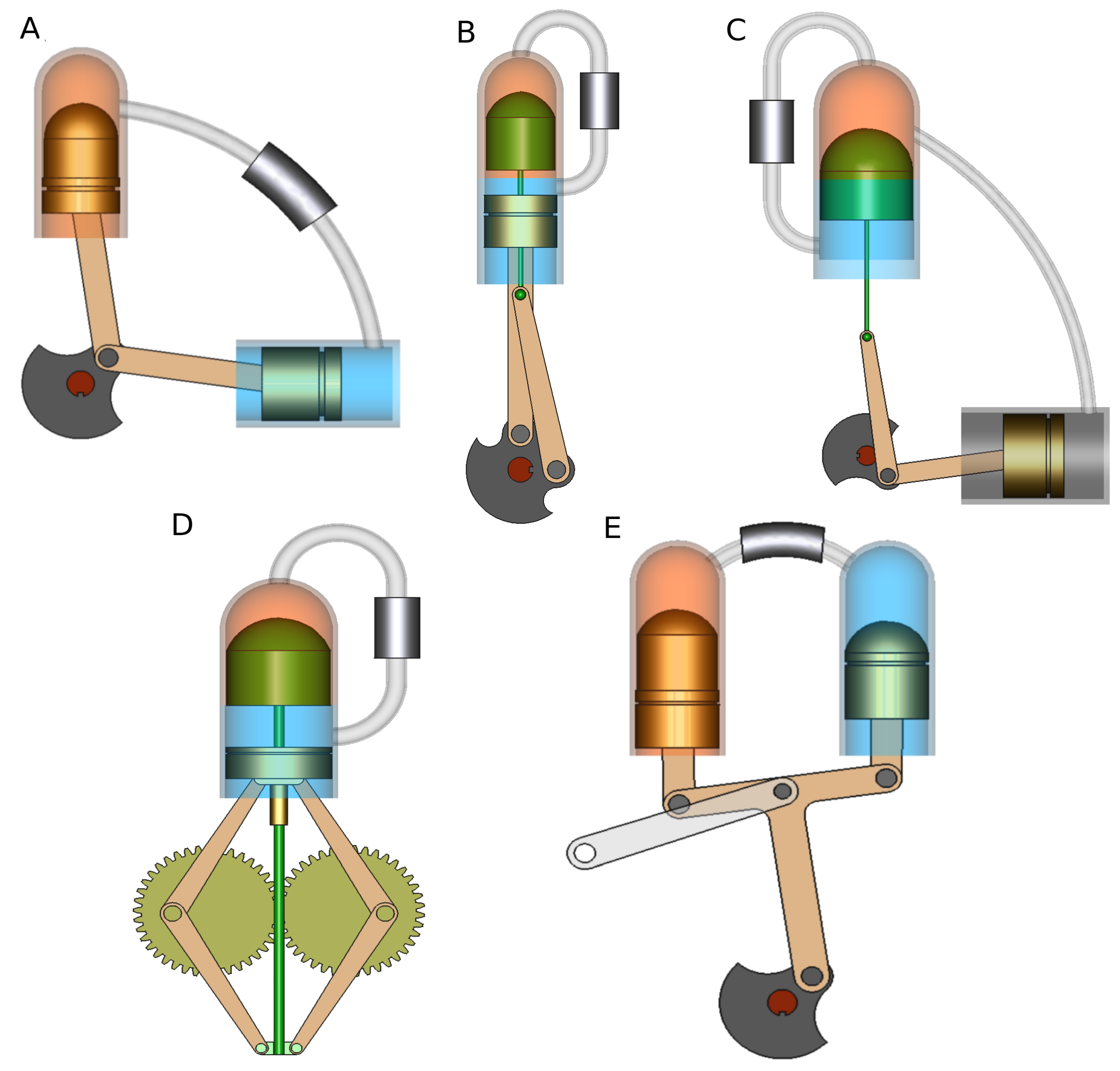
Kinematic Stirling machines can be classified in three main groups: alpha, beta and gamma engines, of which beta engines have two common drive mechanisms, the slider-crank drive and the rhombic drive, and alpha machines commonly use crank drive or Ross yoke. In Figure 1, the five engines studied here can be appreciated. Figure 1A represents an alpha configuration with crank drive. It has two pistons, one for the expansion volume and one for the compression volume, both connected to the same crankshaft. The two cylinders are connected together through a pipe and the regenerator, and form an angle of 90 degrees between them. Figure 1B represents a beta configuration with crank drive. It has piston and displacer within the same cylinder and both are connected to two crank mechanisms phased 90 degrees. Figure 1C is a gamma configuration with crank drive. Piston and displacer are housed within two cylinders phased 90 degrees and connected trough a pipe and a regeneartor. Figure 1D represents a beta configuration with similar characteristics as Figure 1B but a different drive mechanism, a rhombic drive replaces the crank. Figure 1E shows the alpha configuration with Ross yoke instead of a crank drive. For all the figures, the next color nomenclature has been used: Expansion and compression (hot and cold) volumes are represented with transparent red and blue respectively. Golden pistons are sealing pistons and green pistons are displacers. Regenerators are represented with metallic gray cylinders.
In this section these configurations are analyzed using the Schmidt theory and MBD. To develop this analysis in a simple way, the next assumptions are made:
- Zero displacer thickness (no dead volume due to the displacer).
- No dead volume in connection pipes or any other part.
- All the assumptions made by thermodynamics, such as infinite heat transfer time, ideal gas properties, uniform instantaneous gas temperature and pressure, etc.
For all the analysis, the four thermodynamic processes are assumed to be:
- p1: gas compression.
- p2: gas heating.
- p3: work process.
- p4: gas cooling.
2.1. Beta with Crankshaft Drive
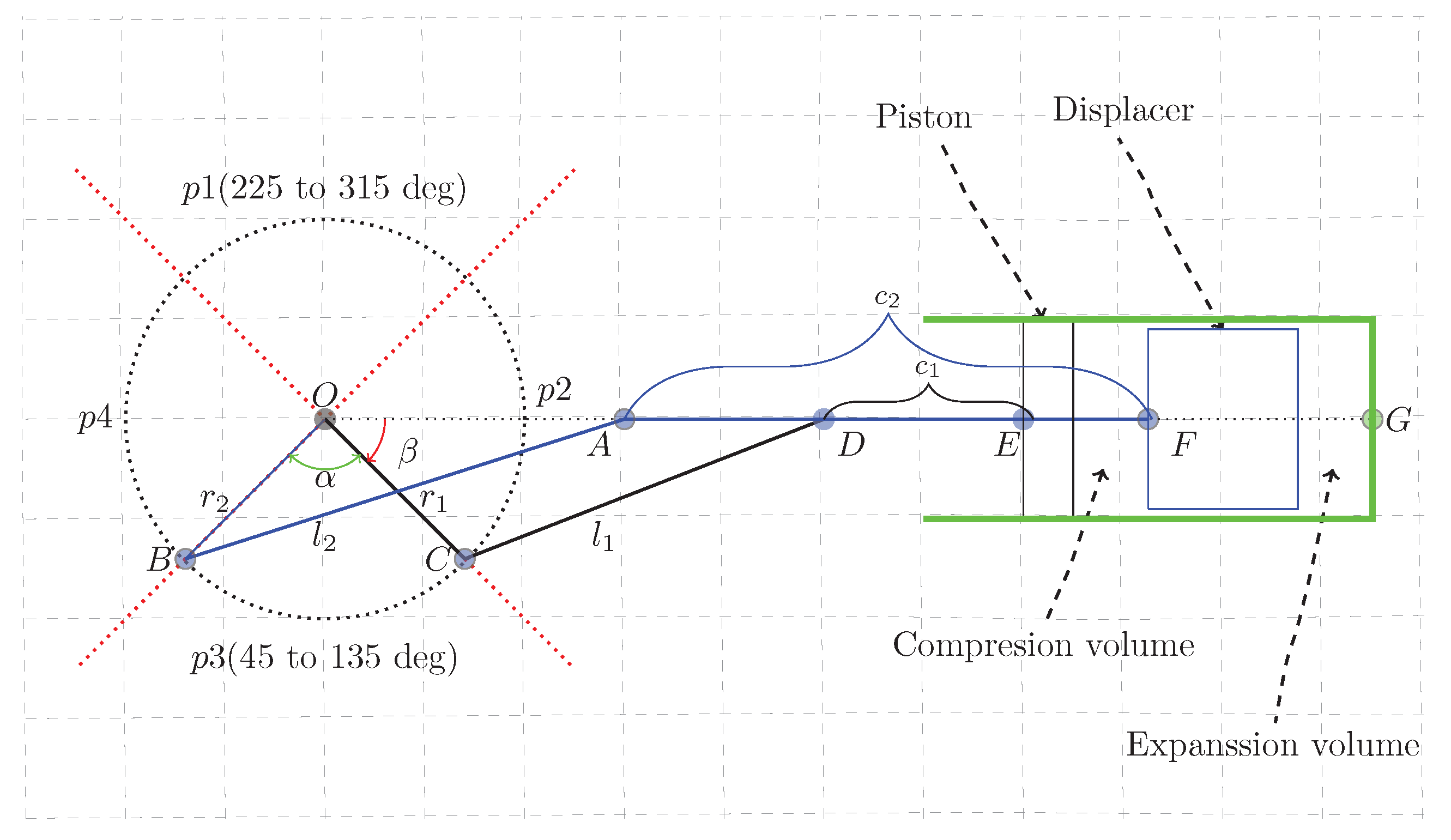
A representation of the beta geometric configuration with crankshaft drive can be seen in Figure 2, where the following nomenclature has been used:
- O point represents the crank rotation center.
- segment represents the power piston crank radius ();
- segment represents the displacer crank radius ();
- segment represents the power piston connecting rod of length.
- segment represents the displacer connecting rod of length.
- segment represents power piston rod of length.
- segment represents displacer yoke rod of length.
- G point represents the displacer top dead center.
- angle represents the phase angle.
- angle represents the crank angle relative to the horizontal.
- are the crank radius for power piston and displacer respectively.
- are the connecting rod lengths for power piston and displacer respectively.
Then, to ensure all the working gas is being displaced, the segment must be:
Cosine law (it is important to note that, since we are interested in the kinematic differences between each configuration and although the original Schmidt theory assumes sinusoidal piston and displacer motions, here we employ the real motion equations as given by the cosine law) applied to and triangles gives us the kinematic equations as functions of crank angle () and referenced to the top dead center G, for the power piston and displacer motions respectively:
Then, assuming the power piston radius to be (), the total volume inside the engine can be expressed as:
The displacer splits the total volume into two, the expansion volume () which is the volume within the hot heat exchanger (for a simple engine using flat heat exchangers, the volumes within the hot and cold heat exchangers are the same as the expansion and compression volumes, respectively), and the compression volume () which is the volume within the cold heat exchanger, these volumes can be expressed as:
Equation (4) has a maximum and a minimum, which represent the maximum and minimum volumes inside the engine. These volumes can be calculated by finding the roots of Equation (7).
which has two solutions ( and ) representing the two crank angles producing the minimum () and maximum () volumes inside the machine:
The engine’s compression ratio () can then be obtained using Equation (10).
In the case of the beta configuration, by solving Equation (7), we find that and , then, the compression ratio can be simply expressed by Equation (11).
Using the ideal gas state equation:
where P is the gas absolute pressure, V it’s volume, it’s molar mass, R the universal gas constant and T the gas absolute temperature. Two state equations can then be posed, one for the expansion volume and one for the compression volume, and given that the working gas mass must be constant (the Stirling cycle is closed), and given Equation (5) for the expansion volume () and Equation (6) for the compression volume (), the next relation for the working gas pressure as a function of the crank angle is derived:
Equation (13) is known as the Schmidt equation, and can be used to calculate the working gas pressure (this calculation is limited by all the thermodynamic assumptions such as infinite heat transfer time and homogeneous gas temperature and pressure. In a real engine, the working gas pressure will be a fraction of the Schmidt pressure) P as a function of the crank angle.
The working gas mass can be calculated from the state equation, using the engine’s initial conditions:
where is the static engine absolute pressure (one atmosphere for non pressurized engines), is the maximum volume as given by Equation (9) ( in the case of the beta engine) and is the room absolute temperature, that is, the temperature at which the engine was first pressurized.
As we already have the total volume, we can now find the engine’s P-V diagram (as predicted by the Schmidt equation) by using Equation (4) in the X axis and Equation (13) in the Y axis.
Finally, the Schmidt indicated work () is given by the area enclosed by the pressure-volume diagram, and can be calculated by subtracting the area under the gas compression P-V curve (from to ) from the area under the gas expansion curve (from to ), using Equation (15).
2.2. Alpha with Crankshaft Drive
Figure 3 represents an alpha machine with crankshaft drive.
For this configuration, the next nomenclature is used:
- O point represents the crank rotation center.
- segment represents the crank of r radius.
- segment represents the expansion piston connecting rod of length.
- segment represents the compression piston connecting rod of length.
- E point represents the expansion piston top dead center.
- D point represents the compression piston top dead center.
- angle represents the phase angle.
- angle represents the crank angle.
- r is the crank radius.
- are the connecting rods lengths.
Then, the next kinematic equations can be derived from the machine’s geometry:
where, to minimize dead volume, and .
The expansion and compression volumes, given the expansion piston radius () and the compression piston radius (), are given by:
and the total gas volume inside the machine:
The maximum and minimum volumes inside the machine (maximum and minimum of Equation (20)) can also be calculated by finding the two zeroes for the next equation:
which leads to two solutions ( and ) representing the two crank angles producing the minimum () and maximum () volumes inside the engine:
and the machine’s compression ratio:
In this case and (to produce easy to visualize graphs, the crank angles for all the configurations are adjusted so that the work process is first plotted, followed by , and ; this is the reason more than one revolution (405 deg) is required to complete one thermodynamic cycle).
The Schmidt equation takes exactly the same form as for the beta engine (Equation (13)) and the machine’s indicated work () is given by Equation (25).
2.3. Gamma with Crankshaft Drive
A crankshaft based gamma machine is represented in Figure 4. The next kinematic equations can be derived from it’s geometry:
where, to avoid dead volume, and . From the above equations, and being the cylinder-displacer radius and the piston radius, the expansion, compression and total volume formulas can be obtained:
In this case, the same procedure used before leads to and , then, the compression ratio is:
2.4. Beta with Rhombic Drive and Alpha With Ross Yoke Mechanism
Beta machines with a rhombic drive and alpha machines with a Ross yoke are also included in the current analysis; however, their kinematic and Schmidt analytical equations are not presented. Instead, an easier method, based on numerical computational simulation, is used to obtain their P-V diagrams and compression ratios. Multi-body dynamics (MBD) software can be used to model a machine of the desired dimensions, and the results can be visualized by animating a CAD model. By this method, the positions and volumes can be obtained as the crank angle changes and pressures calculated according to the Schmidt equation (Equation (13)). In this work, MBDyn 1.6.1 (a free, open souse multi body dynamics simulation software developed at Politecnico di Milano University, Italy; (see: https://www.mbdyn.org/)) in combination with FreeCAD 0.16 (a free and open source CAD modeler developed by a non for profit Free Software community (see: https://www.freecadweb.org/)) are used.
Figure 5 shows a general representation of the beta configuration using a rhombic drive and Figure 6 represents the alpha configuration with Ross yoke drive.
The details of the MBD simulation implementation itself are irrelevant for the conclusions presented in this article, and since different MBD programs can be used and must lead to the same results, these details will not be presented here (for a detailed explanation on how to simulate mechanical systems (e.g., crank-slider mechanisms) with MBDyn, please visit: http://www.sky-engin.jp/en/MBDynTutorial/). Only the resultant P-V diagrams and compression ratios are shown.
3. Kinematic Engines Proposed
Five hypothetical Stirling machines are now posed. They share the following arbitrary geometric characteristics (please note that, provided that the same values are assumed for all the configurations, these can be randomly selected without affecting the final conclusions):
- cm
- cm
- deg
- cm
- cm
- cm
The next design parameters are applied to all the five machines:
- Equation (1) was introduced for the beta configuration to ensure there is one crank angle for which the clearance volume (volume contained between the displacer and the hot heat exchanger) is zero, thus, ensuring there is no dead volume. Then, the displacer kinematic equation (Equation (3)) was derived under this consideration. For our beta engine, this design consideration can be mathematically expressed as:Therefore, at least one crank angle () that determines zero expansion volume () must exist:Then, to ensure the minimum compression volume () during the work process, the same logic must be applied to the distance, that is, the distance between the power piston and the displacer (distance that determines the compression volume):If satisfied, conditions (33) and (34) ensure that: (i) there is no dead volume caused by inadequate scarce swept volume, (ii) that the expansion volume is as big as possible and the compression volume is as small as possible during the work process (p3), and (iii) that the compression volume is as big as possible and the expansion volume is as small as possible during the compression process (p1). To satisfy these two conditions we must adjust the connecting rods lengths. Under this criteria, the next lengths have been selected for our hypothetical engines:
- (a)
- Beta with crankshaft drive:
- cm
- cm
- cm
- cm
- (b)
- Alpha with crankshaft drive:
- cm
- (c)
- Gamma with crankshaft drive:
- cm
- cm
- (c)
- Beta with rhombic drive:
- cm
- cm
- cm
- (c)
- Alpha with Ross yoke:
- cm
- Zero dead volume is assumed within the five machines proposed.
- Perfect regeneration is assumed for the five machines proposed.
Additionally, the next parameters are used for the beta rhombic and alpha Ross yoke proposed machines:
Finally, all the proposed machines are assumed to work under the same conditions:
- kPa
- K
- K (Cold volume temperature)
- K (Hot volume temperature)
For which pressure and temperatures are an arbitrary choice (as for the previous arbitrary dimensions, these values can also be modified without affecting the final conclusions).
4. Compression Ratio as Function of Temperature Difference
From the ideal Stirling cycle, it can be derived that a direct linear relation between the the temperature ratio () and the optimum compression ratio exists. The West equation (Equation (35), retrieved from [16] (p. 103)), shows us there is a direct relation between the applied temperature difference () and the work per cycle that is attainable with a certain Stirling machine. This is due to an increased difference between the expansion pressure and the compression pressure resulting from the incremented that, at the same time, increases the area enclosed by the pressure-volume diagram by enlarging the pressure range. To further increase the work per cycle and optimize the engine for a higher , we also have to increase the power piston swept volume until an optimum point has been reached, the point where the area covered by the pressure-volume diagram is maximized. It is important to remember that the area under the work process can be interpreted in two different ways, as work delivered by the working gas, if the force due to its pressure is higher than the total force applied to the piston “outside face” (remember that work is not just pressure times volume, but also force times distance); or, as work transferred to the working gas if the opposite is true, thus, three compression ratios are possible: First, a too high will turn part of the thermodynamic cycle into a heat pump cycle by the phenomenon just described, reducing the engine’s performance; second, an optimum will extract the maximum work attainable; and third, a too small will reduce the work per cycle by a shortage of swept volume, therefore reducing the engine’s performance.
Due to the assumptions made by the Schmidt theory, which is the ideal isothermal Stirling cycle modified by the machine’s kinematics, it is impossible to use this simple mathematical model (or any other exiting model [25]), to exactly predict the mentioned optimum point that, at the same time, determines the optimum compression ratio for a real machine. However, we can use the ideal cycle to predict an ideal compression ratio () for a given temperature difference. The basic concept behind this can be summarized as: the working gas can exert work over the power piston as far as the magnitude of the force resulting from it’s pressure is higher than the magnitude of the total force applied over the “outside face” of the piston, where both forces are assumed to share direction and have opposite sense. Beyond the point at which the force due to the working gas pressure matches the “outside piston face” total force (including the engine’s load), work should be applied from outside the engine to continue the expansion, thus, reducing the engine’s performance or preventing it from working. During the work process, the point at which the force due to the working gas pressure matches the total force acting on the outside surface of the piston determines the ideal maximum compression ratio, and no engine should be designed with a higher than this maximum which, as seen next, for the ideal thermodynamic cycle is the same as the temperature ratio (). Take for instance the beta machine proposed above, the maximum volume determined by Equation (9) is , and the minimum volume determined by Equation (8) is , which gives us a compression ratio . The engine is assumed to be subject to a temperature difference of . From the Schmidt equation (Equation (13)) the mean cycle pressure can be obtained, resulting in kPa. We can assume, to simplify the analysis to an ideal case, that the engine external gas, the gas on the outside of the power piston, is at a constant pressure equal to the mean thermodynamic cycle pressure; and that the engine works under zero load, thus, no force, except for the constant force due to the external gas pressure and the oscillating force due to the working gas pressure, is exerted over the power piston. Under these conditions, the resultant ideal thermodynamic cycle, depicted in Figure 7, shows that the working gas pressure in the third thermodynamic state (after the work process has finished) is below the mean cycle pressure, which was assumed to be equal to the external gas pressure, thus, work must have been done over the power piston to expand the working gas beyond the point it has already delivered all the work that it can deliver. The engine’s compression ratio is too high for the applied .
Now, let us decrease the maximum volume to keeping all the other values constant (this can be done in a real engine by modifying its geometry or the drive mechanism). The resultant ideal P-V diagram can be appreciated in Figure 8. Note that now the working gas pressure at the third thermodynamic state matches the working gas pressure at the first thermodynamic state which, at the same time, is equal to the the outside constant gas pressure, this means that all the work that the working gas can do has been done, and that no unnecessary further expansion is forced. This sets the ideal (maximum) compression ratio for the current temperature difference to . Based on this, and working with the ideal isothermal Stirling cycle (Boyle’s and Gay-Lussac’s gas laws), one can derive the conclusion that the ideal compression ratio () is exactly the same as the applied temperature ratio:
5. Empirical Compression Ratio
LTD engines are notably sensitive to the adequate , being the reason why designers usually pay special attention when estimating the for LTD machines and, as can be seen by reviewing the literature summarized in Table 1, most of the designers do not even consider the for HTD engines. A direct linear relation between applied temperature difference and an appropriate design compression ratio for LTD engines has been observed in the past. The next empirical formula was proposed by Ivo Kolin [26] (p. 200):
where 1100 is an empirically derived number, obtained by Ivo Kolin from the performance analysis of a number of LTD machines.
As mentioned, a specific formula to calculate the CR for HTD machines does not exist in the published literature. To validate the usability of Kolin’s LTD equation for HTD engines, we have compared it with experimental results from published working Stirling engines (unfortunately, as [27] mentions, data for temperature difference and compression ratio is rarely included in published articles and reports, which has limited the validation of Equation (37) to just six experimental cases). In Table 2, working hot and cold temperatures can be appreciated, along with the compression ratios obtained with Formulas (36) and (37) (for the real working temperatures of each engine), and the actual compression ratio used by the project authors.
To visualize the two variable dependent equations in an easy to interpret two dimensional graph, we can set the cold temperature to a constant value of , which is the mean for all the experimental machines considered, and assume the two equations are function only of the hot temperature , which is the temperature that depends on the specific Stirling engine application (solar energy, biomass, heat recovery, etc.), so that we can compare the two compression ratios with the experimental data. As can be seen in Figure 9, due to the idealizations and assumptions inherent to the ideal cycle, the experimental compression ratio and the compression ratios used by real engines are below the ideal compression ratio .
Note that there is an important difference between the heat exchangers used for LTD and HTD machines. Since usually LTD machines work at low pressures and produce relatively low power to weight and power to size ratio, their heat exchangers are big enough to ensure enough heat transfer (conduction and convection) for the machine’s steady operation, even when simple flat surfaces are used (also, it is important to consider that, for LTD machines, the limiting heat transfer mechanism is the convection, transferring heat between the heat exchangers and the gas, rather than the heat conduction within the material of the heat exchangers [33] (p. 139)). For high pressure and high power to weight and power to size ratio HTD machines, heat exchangers are relatively small compared with the heat flux ratio required for the steady machine operation, and complex increased area heat exchangers are commonly designed and optimized. Also, LTD machines don’t usually include efficient regenerators, whereas most HTD engines include appropriate mechanisms to force the working gas through a high porosity regenerator. Based on this, we can assert that the real working gas temperatures, during the work process and the compression process, will be closer to the hot and cold heat exchanger temperatures, respectively, within HTD engines than within LTD engines. Formula (37), being proposed for and obtained from LTD engines, measuring the heat exchanger’s temperatures rather than the actual gas expansion and compression temperatures, does not take into account the mentioned facts, thus, the LTD formula may limit the work per cycle (due to a shortage of power piston swept volume) and affect the overall performance when used to calculate the compression ratio for a HTD engine, specially if it uses complex heat exchangers and if it works highly pressurized. Formula (37) should be used as an approximation. To find the optimum CR for a specific engine, an empirical optimization must be performed by measuring the performance of the real machine while adjusting its compression ratio.
6. Results
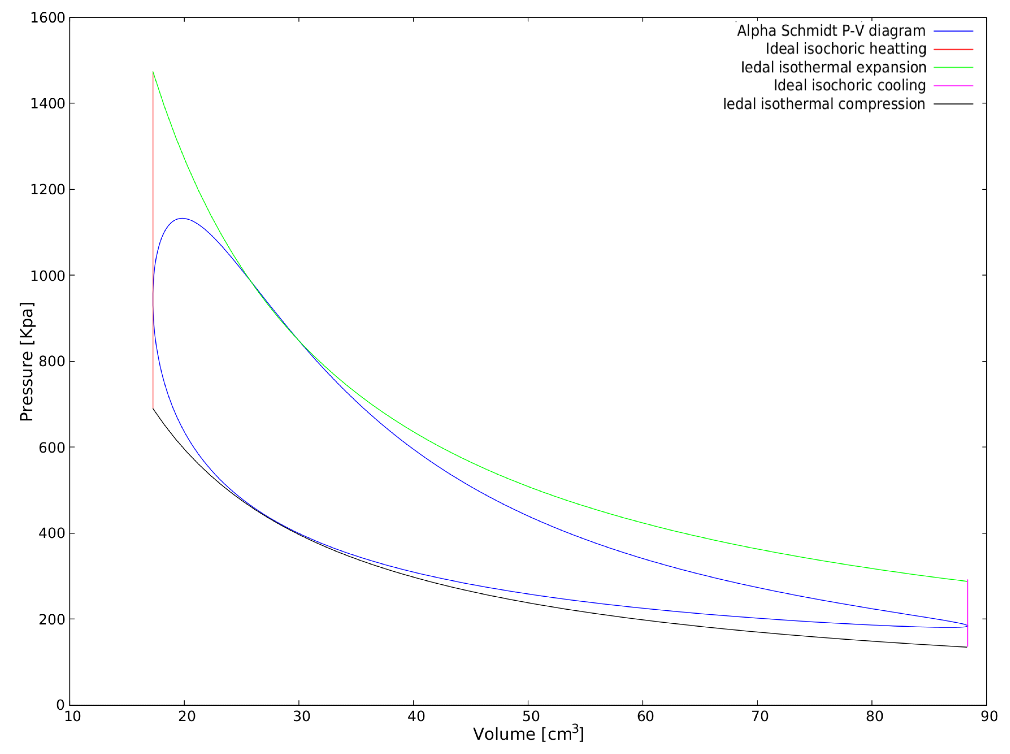
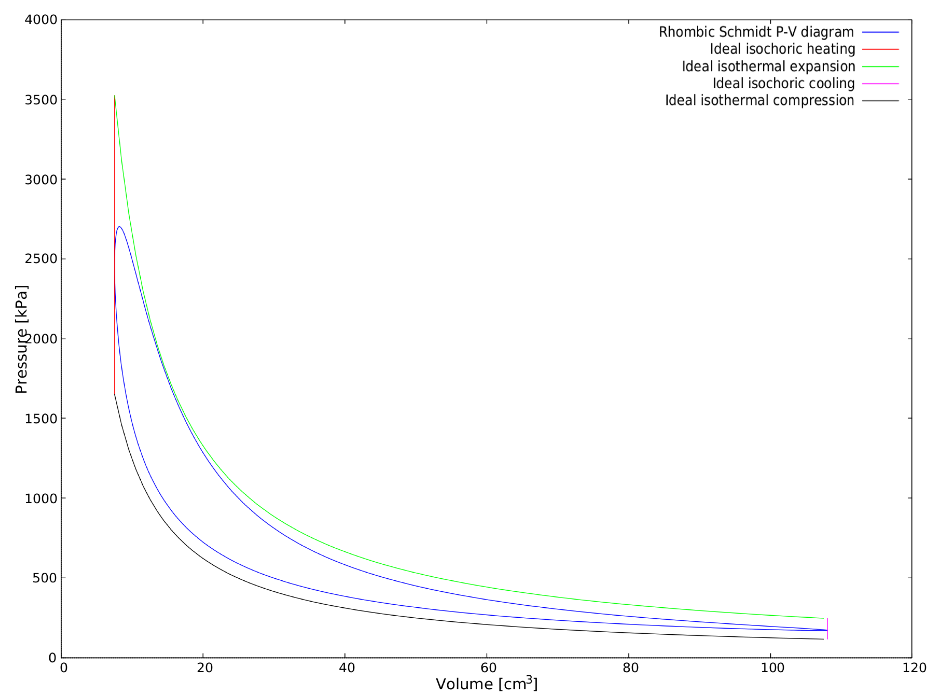
The Schmidt equation (Equation (13)) allows plotting the P-V diagrams shown in Figure 10, Figure 11, Figure 12, Figure 13 and Figure 14 for beta, alpha, gamma, beta rhombic and alpha Ross configurations respectively. The ideal isothermal models as given by the state equation (that is, contrary to what happens with the Schmidt equation, not considering the machine’s kinematics) have also been plotted for comparison.
Table 3 gathers the calculated values for the five proposed engines working under the above mentioned similar conditions. The main parameter considered in the current study, the compression ratio calculated from the machine’s kinematics, is first shown, along with the ideal compression ratio as given by Equation (36) and the compression ratio calculated with Ivo Kolin’s formula (Equation (37)) for the design hot and cold temperatures ( K and K).
7. Discussion
The results obtained demonstrate that, for any Stirling engine, there is a direct relation between the optimum compression ratio and the applied temperature ratio. For the ideal Stirling cycle, the optimum compression ratio is the same as the temperature ratio. For real engines, the concordance between the compression ratio predicted by the low temperature difference equation (equation number (37)) and real HTD engine’s compression ratios (Figure 9), shows that the mentioned equation can be used to calculate the design compression ratio, as a function of the applied hot and cold temperatures, for high temperature difference machines.
The results presented in Table 3 indicate that, under the same conditions, engines of the same dimensions (same piston and/or displacer bore and stroke) but using different configurations and drive mechanisms, produce widely different compression ratios, thus, according with the above mentioned direct relation between the applied temperature difference and the optimum compression ratio, each machine configuration and drive mechanism is more suitable for different applications depending on the temperature difference attainable by the energy source. Of the engines included here, the one that presents higher compression ratio is the alpha with Ross yoke, followed by beta with rohombic drive, alpha with crank drive, beta with crank drive, and gamma with crank drive.
A selection criteria for the most adequate Stirling engine configuration and drive mechanism is then demonstrated: Those configurations and drive mechanisms that allow higher compression ratio must be preferred for applications where high temperature difference is attainable, and those that allow low compression ratio must be used for low temperature difference applications.
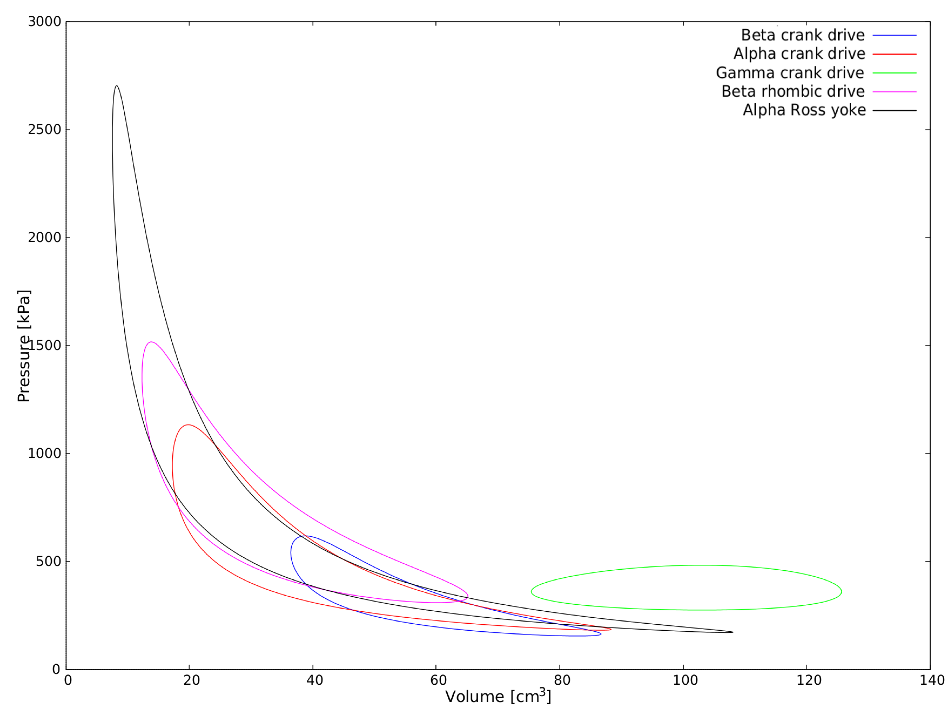
The results obtained are in concordance with the observation, stated by other authors [12] (p. 91), regarding the impossibility of building LTD engines working with alpha or beta rhombic configuration, and that most low machines are of the gamma type configuration. Figure 15 depicts a pattern in the P-V diagrams of all the alpha, beta and gamma machines here considered. Note how they present different minimum and maximum volumes (thus, different ) and different minimum and maximum pressures. Is noticeable that the gamma configuration clearly differs from this pattern. The main difference, as shown in Table 3, is that the gamma configuration allows achieving low compression ratio, thus, according to Equation (37), it is suitable for low temperature difference applications, wherein the other configurations present considerably higher compression ratios, being suitable for higher .
- Alpha machines with Ross yoke are more suitable for high temperature difference applications, among which we may include high concentration ratio solar power (e.g., parabolic dish), nuclear power, high temperature geothermal energy, etc.
- Beta with rhombic drive and alpha with crank-slider machines are more suitable for medium-high temperature difference applications, which may include petrol or liquefied petroleum gas (LPG), medium concentration ratio solar (e.g., central tower or linear Fresnel lenses technologies), etc.
- Beta machines with crankshaft drive are more suitable for medium-low temperature difference applications; examples may include biofuels such as biogas or biodiesel, biomass combustion (agricultural or wood industry waste), etc.
- Only gamma machines are suitable for low and ultra low temperature difference applications, which may include low or zero concentration ratio solar power, low temperature geothermal energy, waste energy recovery, laboratory and educational applications, etc.
It is important to note that any kinematic Stirling engine will run provided that the temperature difference applied is equal or higher than the minimum required for the engine’s compression ratio (e.g., a low CR gamma LTD engine must work under high temperature difference, but a high CR alpha engine cannot work under low temperature difference). This is the the reason why all the applications shown in Table 1 reported successfully running machines despite using different configurations (some of them the inappropriate gamma type) for the same medium application. The results presented here imply that “better results (power to weight and power to size ratio) can be achieved by selecting the appropriate configuration”, and must not be interpreted as “a Stirling engine will not run if the inappropriate configuration is chosen”.
8. Conclusions
One of the factors that has determined the historical failure to introduce Stirling machines as prime movers for several applications is their relative low power to weight ratio and, one of the factors that has reduced the power to weight ratio, is the inappropriate selection of the configuration and drive mechanism. For both, selection of the configuration and calculation of a design compression ratio for high temperature engines, there is a void in the published scientific literature, and no clear selection method can be found in most of the Stirling machine application reports. As consequence, one can still find Stirling engine applications using crank based gamma configurations with low compression ratio for high temperature difference applications. These projects could have reached higher performance by using an appropriate configuration and compression ratio, thus, increasing the chances to succeed. Table 3 shows that, under the same conditions, the different configurations present different CR, being suitable for different applications based on Equation (37) and the empirical data presented in Figure 9. By following the guidelines presented in this article, an appropriate configuration for the specific Stirling application can be selected, potentially leading to a better final prototype and increasing the chances of a successful application.
Author Contributions
Both authors have made significant contributions to the article and worked collectively on the manuscript.
Conflicts of Interest
The authors declare that there are no conflicts of interest related to this work.
References
- To, W.; Lee, P. Energy Consumption and Economic Development in Hong Kong, China. Energies 2017, 10, 1883. [Google Scholar] [CrossRef]
- Warner, K.; Jones, G. The Climate-Independent Need for Renewable Energy in the 21st Century. Energies 2017, 10, 1197. [Google Scholar] [CrossRef]
- Armeanu, D.; Georgeta, V.; Stefan, C. Does renewable energy drive sustainable economic growth? Multivariate panel data evidence for EU-28 countries. Energies 2017, 10, 381. [Google Scholar] [CrossRef]
- Kongtragool, B.; Wongwises, S. A review of solar-powered Stirling engines and low temperature differential Stirling engines. Renew. Sustain. Energy Rev. 2003, 7, 131–154. [Google Scholar] [CrossRef]
- Meybodi, M.A.; Behnia, M. Australian coal mine methane emissions mitigation potential using a stirling engine-based CHP system. Energy Policy 2013, 62, 10–18. [Google Scholar] [CrossRef]
- Mancini, T.; Heller, P.; Butler, B.; Osborn, B.; Schiel, W.; Goldberg, V.; Buck, R.; Diver, R.; Andraka, C.; Moreno, J. Dish-Stirling Systems: An Overview of Development and Status. J. Sol. Energy Eng. 2003, 125, 135–151. [Google Scholar] [CrossRef]
- Boutammachte, N.; Knorr, J. Field-test of a solar low delta-T Stirling engine. Solar Energy 2012, 86, 1849–1856. [Google Scholar] [CrossRef]
- Rey, G.; Ulloa, C.; Miguez, J.L.; Arce, E. Development of an ICE-based micro-CHP system based on a stirling engine; methodology for a comparative study of its performance and sensitivity analysis in recreational sailing boats in different European climates. Energies 2016, 9, 239. [Google Scholar] [CrossRef]
- Toro, C.; Lior, N. Analysis and comparison of solar-heat driven Stirling, Brayton and Rankine cycles for space power generation. Energy 2017, 120, 549–564. [Google Scholar] [CrossRef]
- Song, C.; Liu, Q.; Ji, N.; Deng, S.; Zhao, J.; Kitamura, Y. Advanced cryogenic CO2 capture process based on Stirling coolers by heat integration. Appl. Therm. Eng. 2017, 114, 887–895. [Google Scholar] [CrossRef]
- Araoz, J.A.; Salomon, M.; Alejo, L.; Fransson, T.H. Numerical simulation for the design analysis of kinematic Stirling engines. Appl. Energy 2015, 159, 633–650. [Google Scholar] [CrossRef]
- Wang, K.; Sanders, S.R.; Dubey, S.; Choo, F.H.; Duan, F. Stirling cycle engines for recovering low and moderate temperature heat: A review. Renew. Sustain. Energy Rev. 2016, 62, 89–108. [Google Scholar] [CrossRef]
- Gopal, V.K.; Duke, R.; Clucas, D. Active stirling engine. In Proceedings of the IEEE Region 10 Annual International Conference, Singapore, 23–26 January 2009; pp. 1–6. [Google Scholar]
- Tavakolpour-Saleh, A.R.; Zare, S.H.; Bahreman, H. A novel active free piston Stirling engine: Modeling, development, and experiment. Appl. Energy 2017, 199, 400–415. [Google Scholar] [CrossRef]
- Conroy, G.; Duffy, A.; Ayompe, L.M. Economic, energy and GHG emissions performance evaluation of a WhisperGen Mk IV Stirling engine u-CHP unit in a domestic dwelling. Energy Convers. Manag. 2014, 81, 465–474. [Google Scholar] [CrossRef]
- Walker, G.; Senft, J.R. Free-Piston Stirling Engines; Springer: Berlin/Heidelberg, Germany, 1985; pp. 23–99. [Google Scholar]
- Fedele, L.; Nasco, V.W.G. Research and development of a biomass fired Ringbom-Stirling engine. In Proceedings of the Eight International Stirling Engine Conference and Exhibition, Ancona, Italy, 27–30 May 1997. [Google Scholar]
- Podesser, E. Small scale cogeneration in biomass furnaces with a Stirling engine. In Proceedings of the Eight International Stirling Engine Conference and Exhibition, Ancona, Italy, 27–30 May 1997. [Google Scholar]
- Liu, B.; Li, L. Design of a domestic free piston Stirling electric power system. In Proceedings of the Eight International Stirling Engine Conference and Exhibition, Ancona, Italy, 27–30 May 1997. [Google Scholar]
- Carlsen, H. Field test of 40kW Stirling engine for wood chips. In Proceedings of the Eight International Stirling Engine Conference and Exhibition, Ancona, Italy, 27–30 May 1997. [Google Scholar]
- Pålsson, M.; Carlsen, H. Development of a wood powder fuelled 35 kW Stirling CHP unit. In Proceedings of the 11th ISEC (International Stirling Engine Conference), Rome, Italy, 19–21 November 2003; pp. 221–230. [Google Scholar]
- Damirchi, H.; Najafi, G.; Alizadehnia, S.; Mamat, R.; Nor Azwadi, C.S.; Azmi, W.H.; Noor, M.M. Micro Combined Heat and Power to provide heat and electrical power using biomass and Gamma-type Stirling engine. Appl. Therm. Eng. 2016, 103, 1460–1469. [Google Scholar] [CrossRef]
- Beck Peter, C.K. Decentralized generation of energy out of biomass using enhanced technologies. In Proceedings of the 11th International Stirling Engine Conference, Rome, Italy, 19–21 November 2003. [Google Scholar]
- Arashnia, I.; Najafi, G.; Ghobadian, B.; Yusaf, T.; Mamat, R.; Kettner, M. Development of Micro-scale Biomass-fuelled CHP System Using Stirling Engine. Energy Procedia 2015, 75, 1108–1113. [Google Scholar] [CrossRef]
- Ahmadi, M.H.; Ahmadi, M.A.; Pourfayaz, F. Thermal models for analysis of performance of Stirling engine: A review. Renew. Sustain. Energy Rev. 2017, 68, 168–184. [Google Scholar] [CrossRef]
- Kolin, I. Stirling Motor: History-Theory-Practice; Inter University Center: Dubrovnik, Croatia, 1991. [Google Scholar]
- Cipri, K.; Lucentini, M.; Kolin, I. Stroke Volume Depending Upon Working Temperature. In Proceedings of the 11th International Stirling Engine Conference, Rome, Italy, 19–21 November 2003; University of Zagreb: Zagreb, Croatia, 2003; Volume D. [Google Scholar]
- Cinar, C.; Yucesu, S.; Topgul, T.; Okur, M. Beta-type Stirling engine operating at atmospheric pressure. Appl. Energy 2005, 81, 351–357. [Google Scholar] [CrossRef]
- Stouffs, P. Design of a 1kWe Stirling engine for solar CHP. In Proceedings of the European Stirling Forum 2000, Osnabrück, Germany, 22–24 February 2000. [Google Scholar]
- Huang, S. Developing and Improving a Small Stirling Engine for Educational Purposes. In Proceedings of the 13th International Stirling Engine Conference, Tokyo, Japan, 24–26 September 2007. [Google Scholar]
- Viebach, S. Simulation and Development of a Stirling Eengine for a small Cogeneration Unit. In Proceedings of the Eight International Stirling Engine Conference and Exhibition, Ancona, Italy, 27–30 May 1997. [Google Scholar]
- Jiri, M. New Cconstruction of the Stirling Engine. In Proceedings of the 11th International Stirling Engine Conference, Rome, Italy, 19–21 November 2003. [Google Scholar]
- Clucas, D.; Egas, J. Additive Manufactured Functional Prime Mover. Energy Procedia 2017, 110, 136–142. [Google Scholar] [CrossRef]
Figure 1.
The five configurations considered in this study.

Figure 2.
Beta configuration with crankshaft drive.

Figure 3.
Alpha configuration with crankshaft drive.
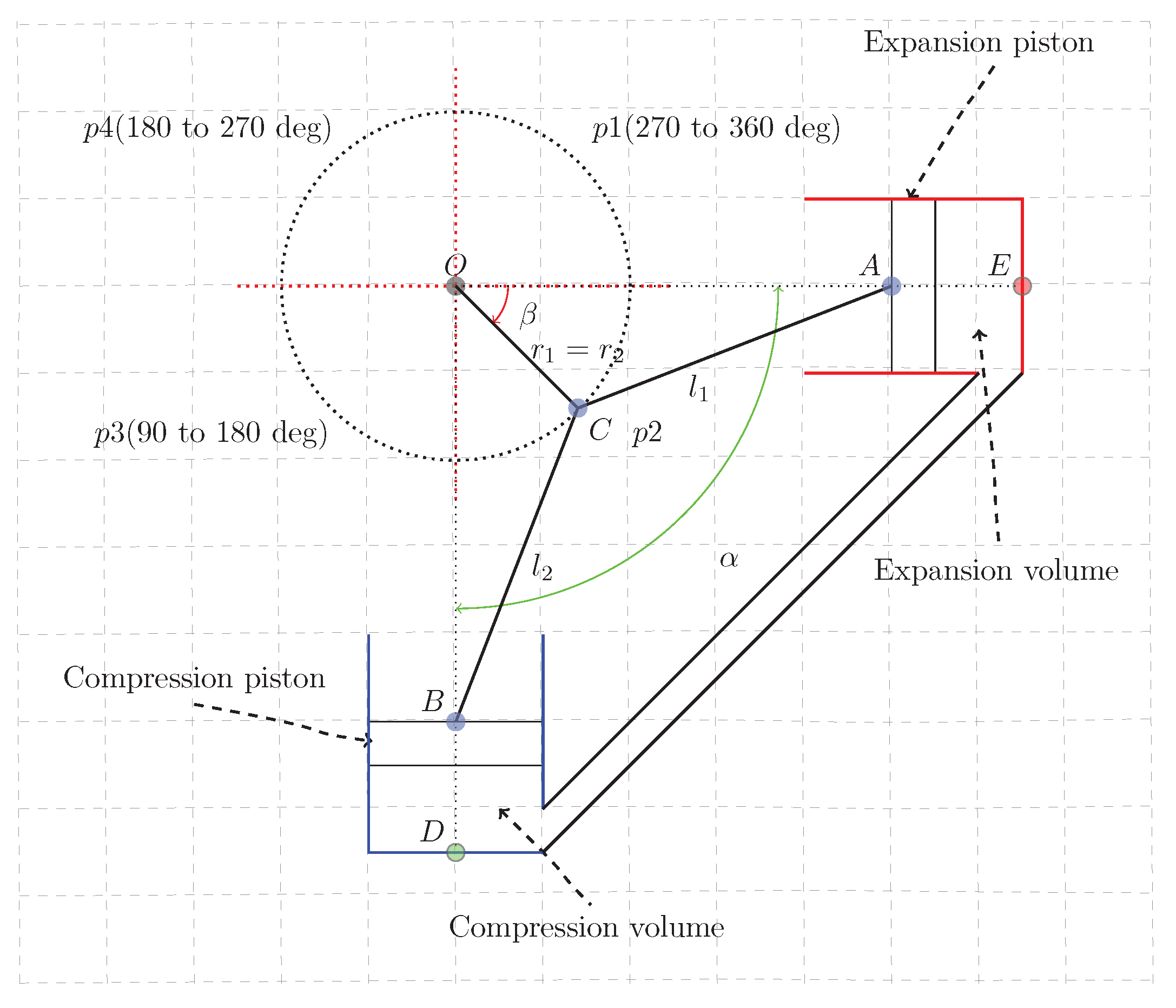
Figure 4.
Gamma configuration with crankshaft drive.
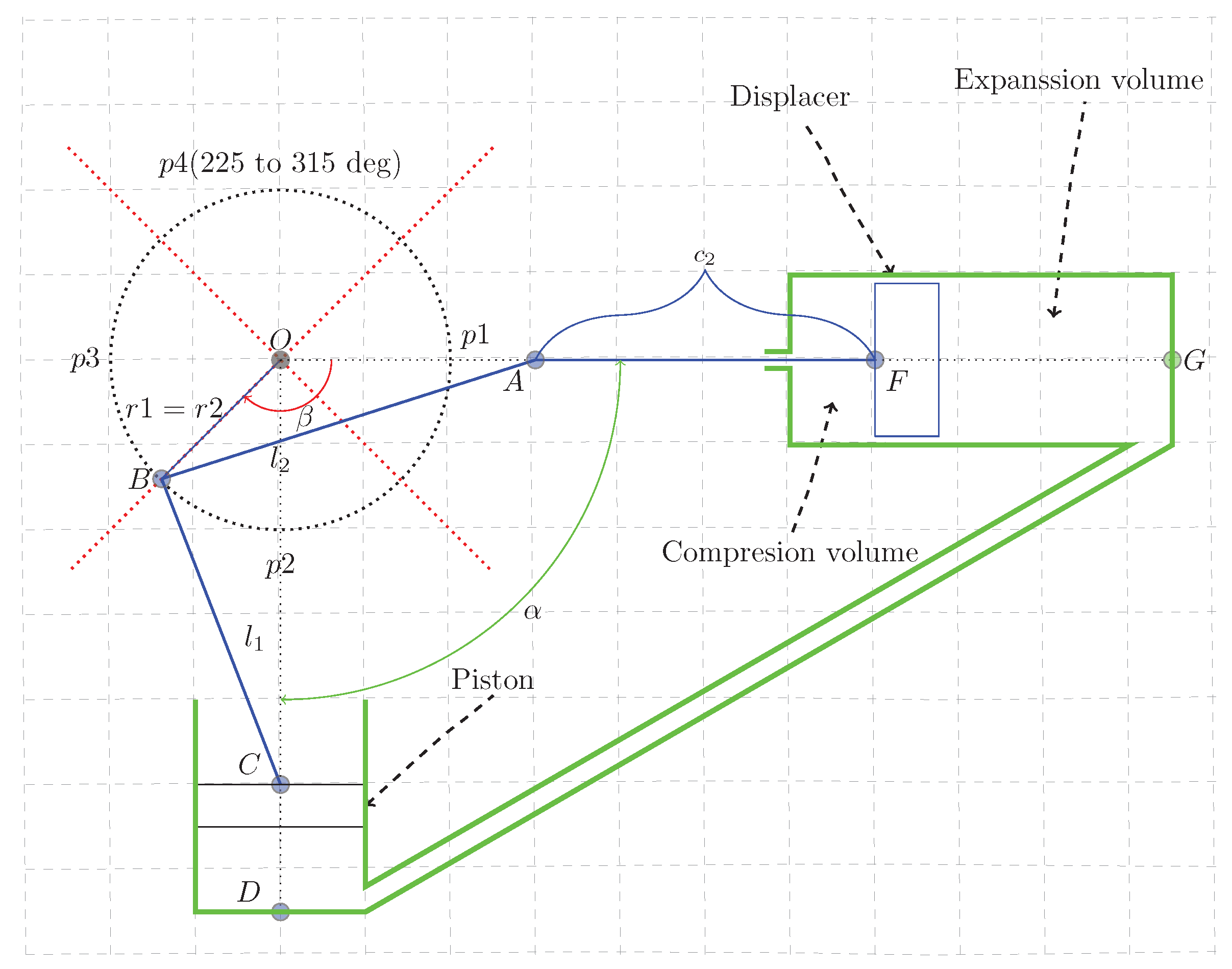
Figure 5.
Beta configuration with rhombic drive.
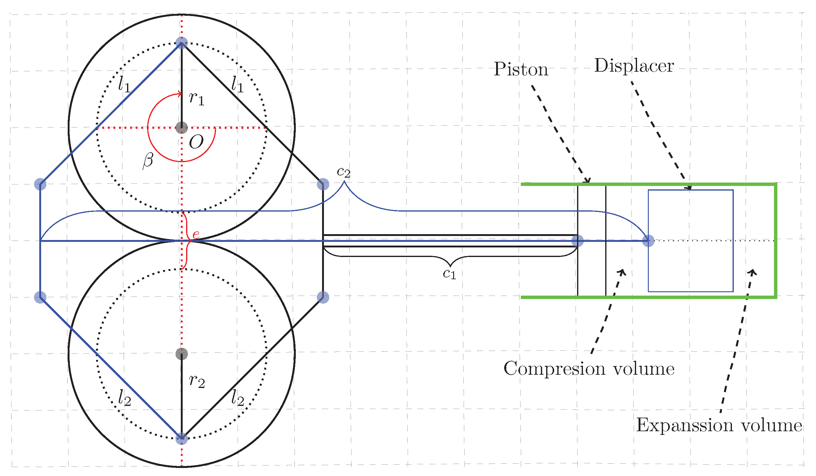
Figure 6.
Alpha configuration with Ross yoke.
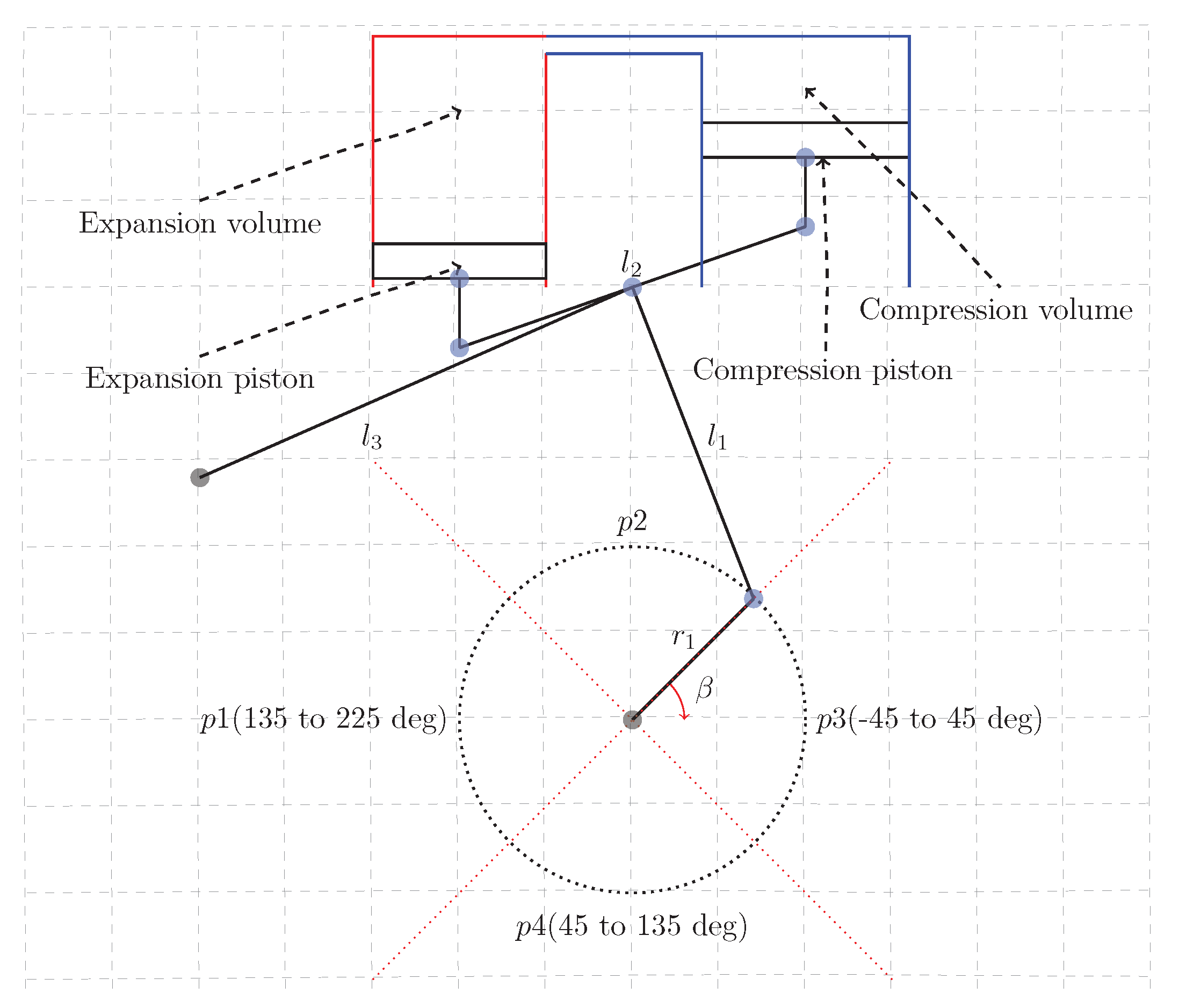
Figure 7.
The proposed beta engine has a too big for the applied .
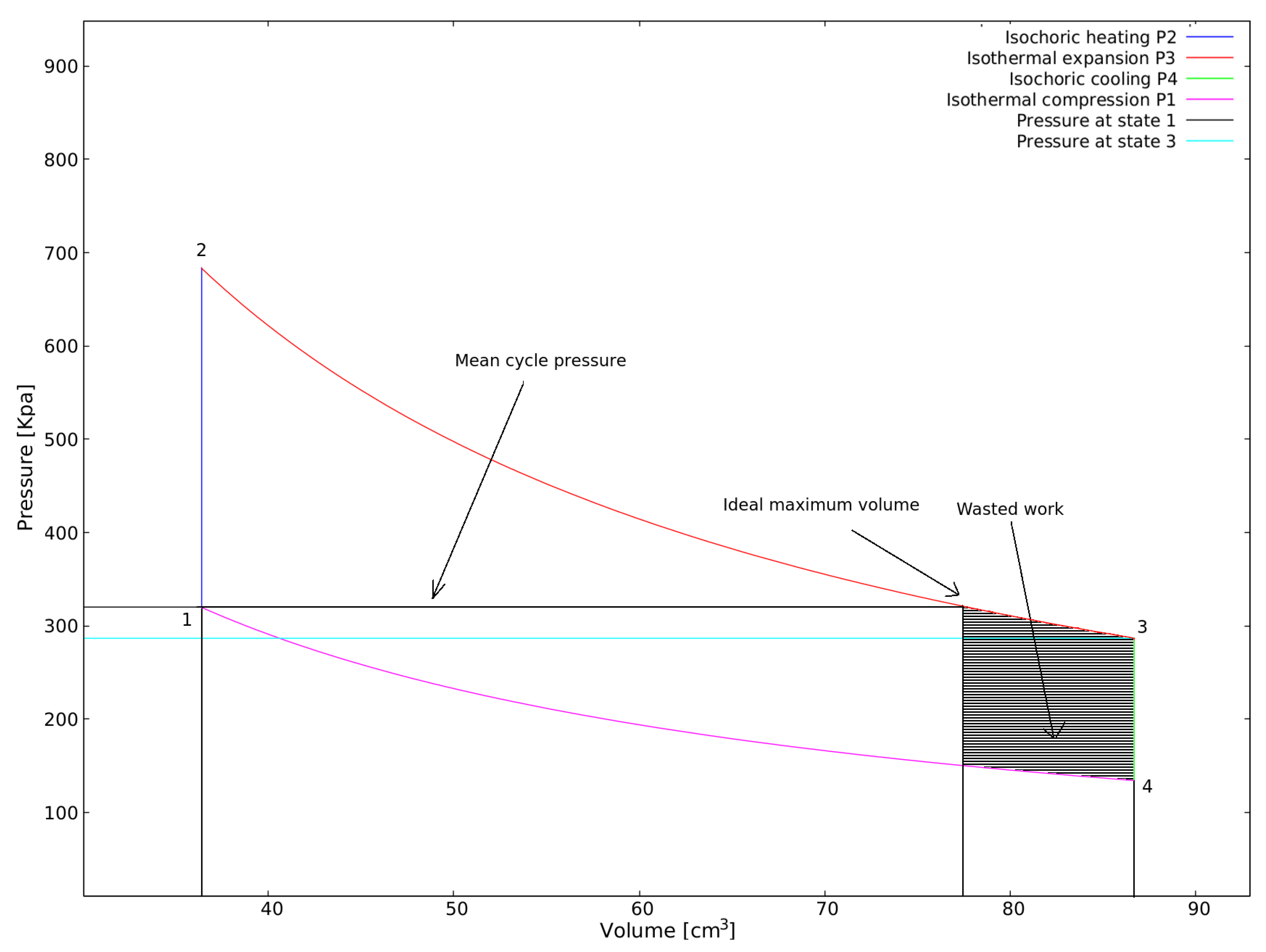
Figure 8.
The ideal for the proposed beta machine.
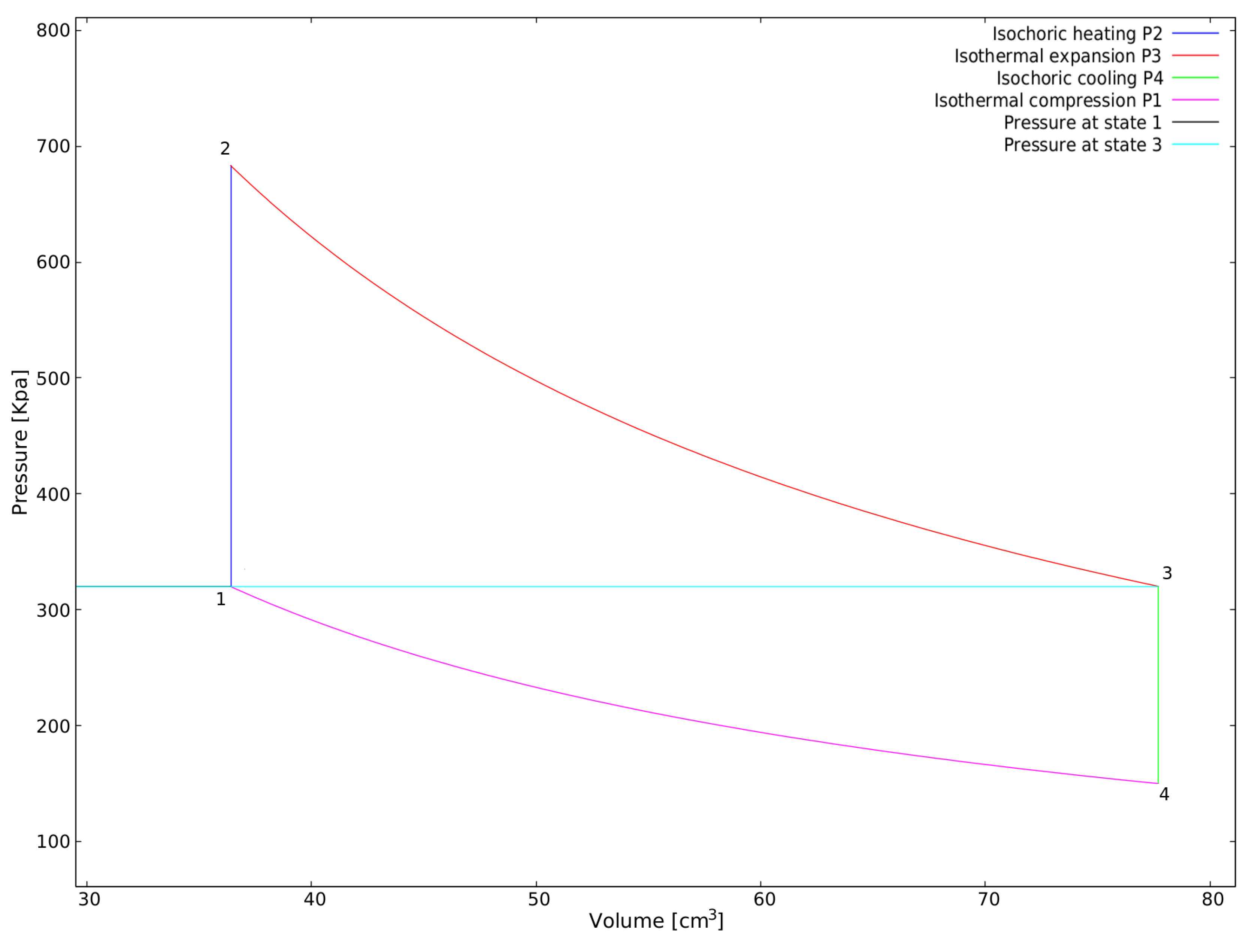
Figure 9.
Ideal (), Kolin’s experimental low temperature difference (LTD) () and experimental high temperature difference (HTD) engine’s .
Figure 9.
Ideal (), Kolin’s experimental low temperature difference (LTD) () and experimental high temperature difference (HTD) engine’s .
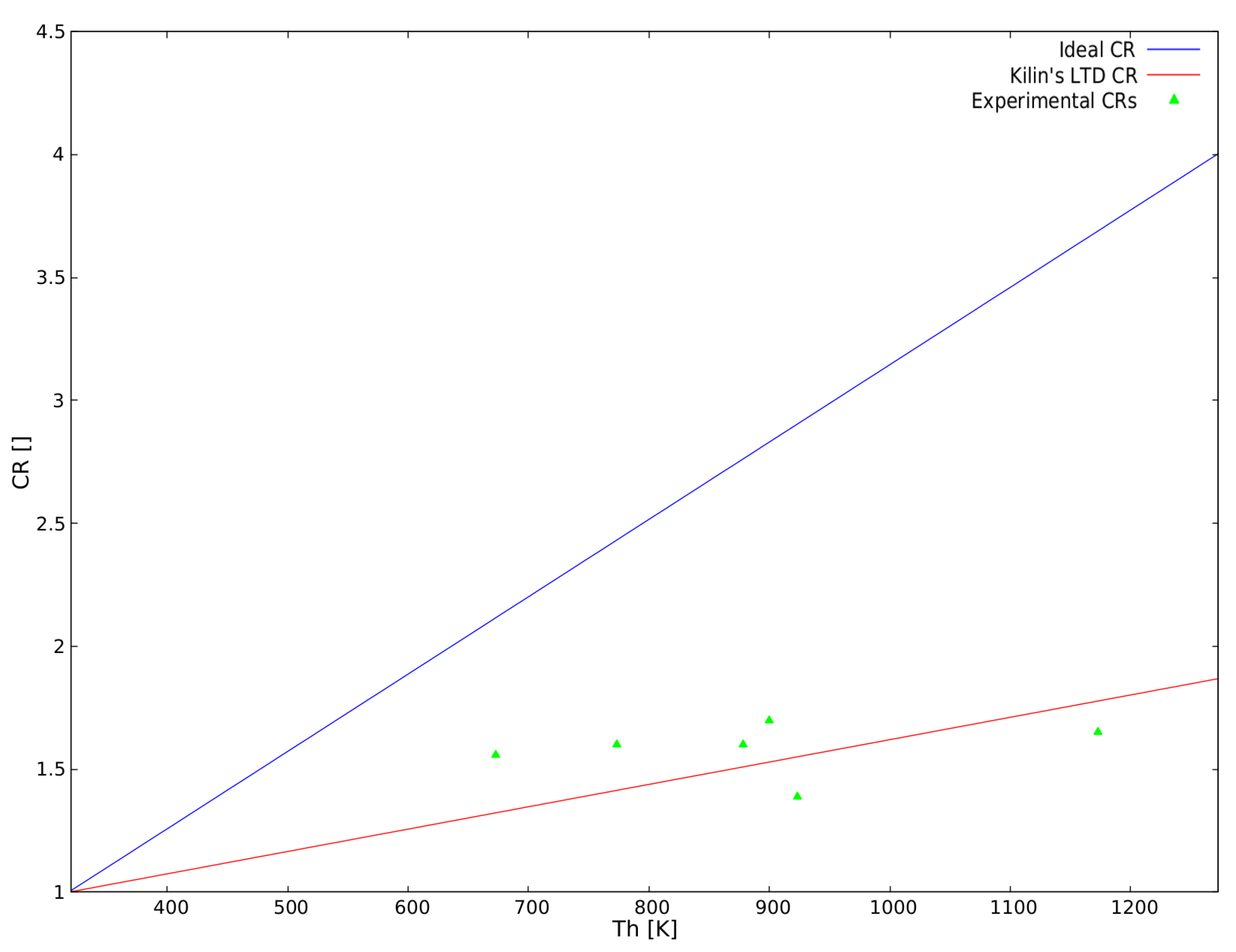
Figure 10.
Beta with crank P-V diagrams.
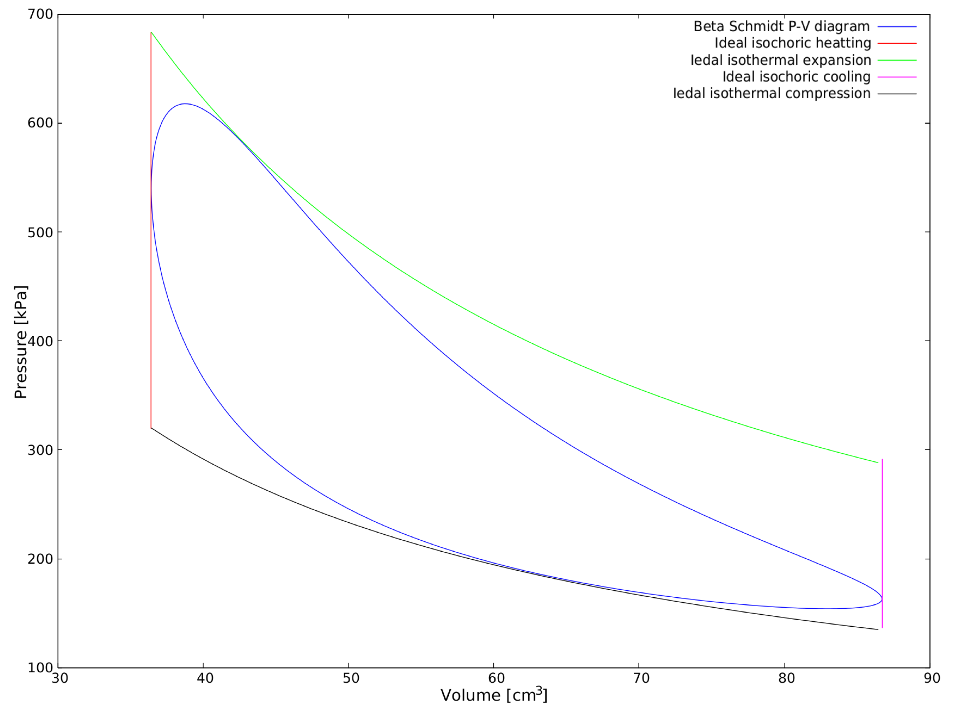
Figure 11.
Alpha with crank drive P-V diagrams.

Figure 12.
Gamma with crank P-V diagrams.
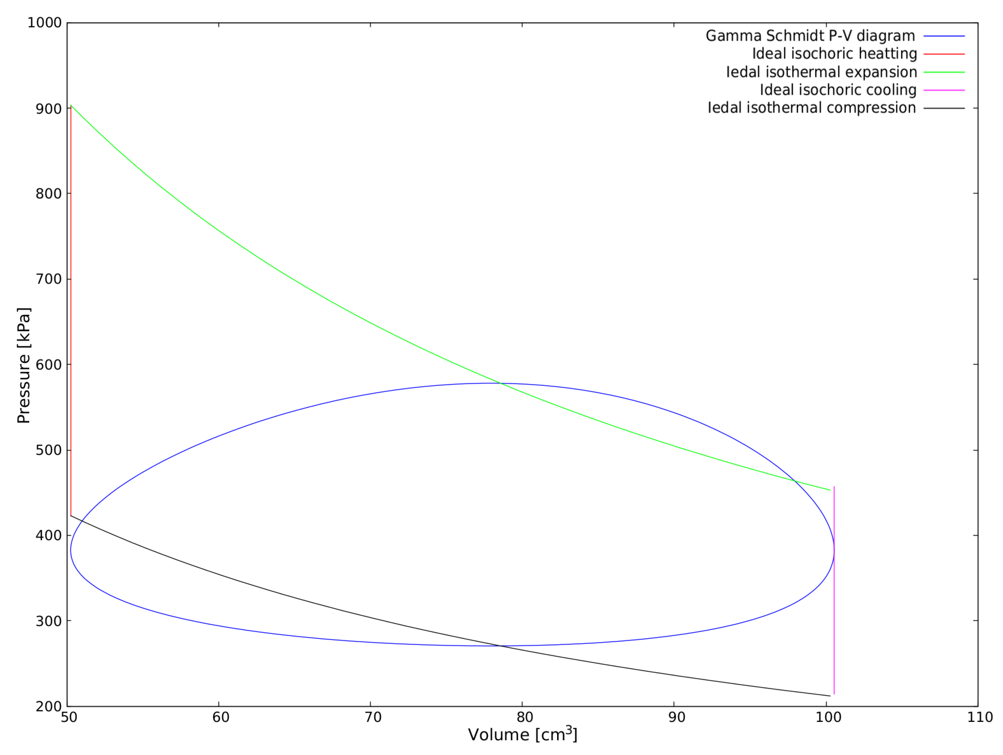
Figure 13.
Beta with rhombic drive P-V diagrams.
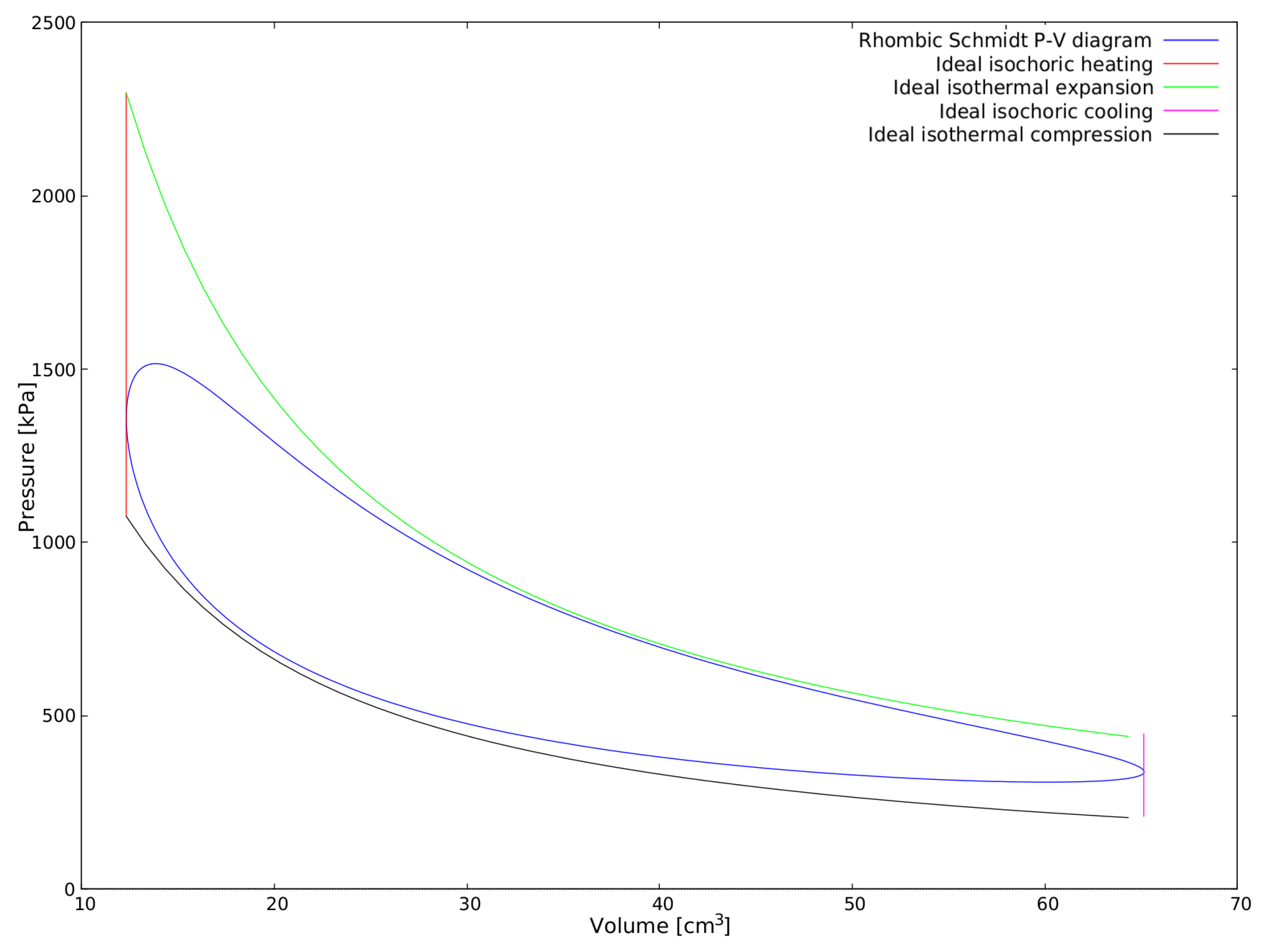
Figure 14.
Alpha with Ross yoke P-V diagrams.

Figure 15.
P-V diagrams comparison.

Table 1.
Different configurations are applied to meet similar objectives.
| Project Title | Ref. | Focus | Engine Configuration |
|---|---|---|---|
| Research and development of a biomass fired Ringbom-Stirling engine | [17] | Low technology users in developing countries | Hybrid (free displacer) |
| Small scale cogeneration in biomass furnaces with a Stirling engine | [18] | District heat plants working with biomass | Alpha type adapted from a motorcycle engine |
| Design of a domestic free piston Stirling-electric power system | [19] | Remote regions in developing countries | Free piston |
| Field test of 40 kW Stirling engine for wood chips | [20] | Decentralized CHP and CO reduction | Alpha double acting four cylinder |
| Development of a wood powder fueled 35 kW Stirling CHP unit | [21] | Blocks of flats, schools, local heat production plats, woody industry. | Double acting four cylinders alpha |
| Micro Combined Heat and Power to provide heat and electrical power using biomass and Gamma-type Stirling engine | [22] | Micro co generation | Gamma type |
| Descentralized generation of energy out of biomass using enhaced technologies | [23] | Waste wood energy recovery | SOLO161 with adapted heat exchanger. |
| Development of micro-scale biomass-fuelled CHP system using Stirling Engine | [24] | Biomass—wood powder | Gamma type. |
Table 2.
Real engine’s compared with the calculated .
| Engine | Experimental | ||||
|---|---|---|---|---|---|
| 5 W beta with crank drive [28]. | 1173 | 303 | 3.9 | 1.8 | 1.65 |
| 1 kW beta with rohombic drive [29]. | 900 | 330 | 2.7 | 1.5 | 1.7 |
| 15 W crank based beta [30]. | 773 | 293 | 2.64 | 1.44 | 1.6 |
| 417 W crank based beta [31]. | 923 | 343 | 2.69 | 1.53 | 1.39 |
| 0.9 kW beta with innovative drive [32]. | 673 | 323 | 2.10 | 1.31 | 1.65 |
| 1 kW solar powered alpha [27]. | 878 | 318 | 2.75 | 1.50 | 1.60 |
Table 3.
Compression ratios for the analyzed engines.
| Beta with crank drive | 2.33 | 2.14 | 1.41 |
| Alpha with crank drive | 5.12 | 2.14 | 1.41 |
| Gamma with crank drive | 2.00 | 2.14 | 1.41 |
| Beta with rhombic drive | 5.28 | 2.14 | 1.41 |
| Alpha with Ross yoke | 14.33 | 2.14 | 1.41 |
© 2018 by the authors. Licensee MDPI, Basel, Switzerland. This article is an open access article distributed under the terms and conditions of the Creative Commons Attribution (CC BY) license (http://creativecommons.org/licenses/by/4.0/).
Share and Cite
MDPI and ACS Style
Egas, J.; Clucas, D.M. Stirling Engine Configuration Selection. Energies 2018, 11, 584. https://doi.org/10.3390/en11030584
AMA Style
Egas J, Clucas DM. Stirling Engine Configuration Selection. Energies. 2018; 11(3):584. https://doi.org/10.3390/en11030584
Chicago/Turabian StyleEgas, Jose, and Don M. Clucas. 2018. "Stirling Engine Configuration Selection" Energies 11, no. 3: 584. https://doi.org/10.3390/en11030584
Note that from the first issue of 2016, this journal uses article numbers instead of page numbers. See further details here.