Multiarea Voltage Controller for Active Distribution Networks


Dipartimento di Ingegneria Elettrica e dell’Informazione, Politecnico di Bari, Via Re David, 200, 70125 Bari, Italy
*
Author to whom correspondence should be addressed.
Energies 2018, 11(3), 583; https://doi.org/10.3390/en11030583
Submission received: 2 February 2018
/
Revised: 28 February 2018
/
Accepted: 5 March 2018
/
Published: 7 March 2018
(This article belongs to the Section F: Electrical Engineering)
Abstract
:The aim of this paper was to develop a multi-area decentralized controller for improving the voltage profile of large active distribution networks. Voltages at control buses of each area are kept as close as possible to their reference values by managing the reactive power of distributed generators within the same areas. Moreover, in order to avoid exchanging a considerable amount of data on more or less large portions of the network, the proposed methodology adopted an equivalent reduced network for each area. This equivalent network model is seen at control buses and nodes where distributed generation units are connected. With this simplification, each area controller will have to evaluate simultaneously, the unknown parameters of the reduced network and the optimal control laws for the voltage profile optimization of its control area. To comply with this exigency, a multi-objective optimization problem was formulated. The solution of this problem formulation was found by adopting an algorithm operating in the continuous time domain. Test results are provided on a 49-bus distribution network, demonstrating the effectiveness of the developed methodology.
1. Introduction
Over the last decade, many research efforts have been carried out to overcome several issues limiting the full exploitation of Distributed Generators (DGs) into actual distribution networks. In fact, these systems are usually operated in such a way that DG resources can create big problems ranging from voltage rise, energy losses, and system restoration in case of faults.
The same DG units can offer a viable solution to these issues, since depending on their own characteristics and location can help to improve the power quality of distribution systems [1]. For this reason, several research efforts have been carried out to report on this topic, giving rise to a wide range of solutions that can be classified into two main categories. The first category is related to those techniques aimed at minimizing the negative effects of DGs integration by choosing their optimal size and location. In particular, papers [2,3,4] suggest a procedure aimed at minimizing active power losses on the distribution system by optimally sizing and placing DG units. The solution of this optimization problem can be found by adopting algorithms based on the branch exchange technique [2], the decision making approach [3], the voltage sensitivity index (VSI) analysis [4], and the Particle Swarm Optimization (PSO) [5,6,7].
Other papers investigate the inherent ability of DG inverters to provide reactive power for minimizing system losses [8,9,10,11,12] or for optimizing the network voltage profile [13,14,15,16,17,18,19,20,21,22,23,24,25,26]. With the aim of obtaining a flat voltage profile, papers [13,14,15,16,17] develop a central controller able to keep nodal voltages within an acceptable range. Although these controllers can give rise to better performance than decentralized ones, their need of a capillary telecommunication infrastructure may be an obstacle to their practical implementation into control centers operating in real time. With the aim to reduce the communication burden, decentralized controllers were proposed in [18,19,20,21]. These controllers are based on a hierarchical control structure based on intelligent and cooperative smart entities. Moreover, in order to overcome possible conflictual operations between all controllers, hierarchical decentralized controllers were suggested in [22,23,24,25,26]. The basic idea of these papers is to split the overall distribution network into several areas whose voltage profile is independently controlled. Although these procedures have been shown to be effective, the mechanism to form the control areas is strictly dependent on the operating point of the network and thus, they need to be continuously updated.
Following the purpose of developing independent voltage area controllers, in this paper a decentralized controller based on a structural decomposition method has been developed. This approach guarantees that identified control areas remain the same until a change in the network topology occurs. By controlling the reactive power sources within each area, the voltage area controller keeps voltages at control buses as close as possible to their reference values. Each area controller evaluates its control actions by solving an optimization problem based on local information, without requiring information of neighboring areas. In this sense, active and reactive powers as well as voltage magnitudes at generation and control buses are used to build an equivalent reduced network seen at these nodes. With this simplification, area controllers are relieved of the computational burden and a parallel computation can be implemented.
Several computer simulations have been performed on an LV distribution network embedding several photovoltaic plants. Results confirm the effectiveness of the proposed methodology and its aptitude to control the network in real time.
This paper is organized as follows: Section 2 outlines the methodology for network partitioning and selection of control buses. Section 3 presents the proposed voltage control methodology and its practical implementation. Section 4 reports some computer simulations performed on an LV distribution network embedding several photovoltaic plants. Section 5 discusses the results and Section 6 concludes the paper.
2. Network Partitioning and Control Bus Selection
The aim of this section is to show how a distribution network can be partitioned into weakly connected sub-networks, so that a closed loop voltage control of each of them can be implemented. Each area should contain at least one control bus where the voltage can be controlled through the reactive power provided by internal DGs.
2.1. Partitioning Procedure
We assume that the system to be partitioned consists of N nodes. In order to identify the weakly coupled subsystems, we applied the structural decomposition method originally developed for transmission networks [27]. This technique is based on the voltage sensitivities and thus needs the evaluation of the voltage coupling degree between network nodes. This information can be derived from the inverse of the Jacobian sub-matrix:
where is the -dimensional sub-matrix, whose elements represent a measure of the sensitivity of nodal voltages with regard to nodal reactive power injections. Therefore, these values can be considered as a good measure of the coupling factor among area nodes. We normalized such coupling factors with regard to the largest one, as follows:
where:
where is the generic element of the matrix.
The resulting -dimensional matrix , whose entries are normalized coupling factors , gives a quantitative measure of the connection level between any pair of nodes. Coupling factors are not reciprocal, i.e., , gives rise to a no symmetrical matrix , even if differences between and are exiguous. Therefore, from a mathematical point of view, can be expressed as follows:
where and represent, respectively, the symmetrical and asymmetrical part of the coupling matrix . In order to simplify the problem, only the symmetrical part of is considered.
In order to perform the recognition of coupled nodes of an area a threshold, , is chosen for the interaction strength. In doing this, the membership of one node to an area is determined by the following binary information:
The choice of implies the identification of one or more areas and thus it must be chosen carefully. In fact, if smaller values of are assumed, the overall system will be identified by one or few areas. On the contrary, if approaches the unitary value, the system will be divided into many areas, at most one area for each node. The resulting sparsified matrix , whose elements are , must be permutated as in [27] obtaining a block diagonal matrix where each block corresponds to a group of coherent nodes.
2.2. Pilot Bus Selection
Once the areas are identified, one or more control buses will be selected for each of them. This selection will be made among those buses exhibiting the highest values of coupling factors. For this reason, the coupling degree among any pair of area nodes must be taken into account.
We assume to have identified M areas and that each of them consists of NM buses. In order to give a measure of how much a generic h-th bus has strength with regard to all other area nodes, the following performance index is defined for each area:
In other words, gives a measure of how much a generic h-th node is able to influence the area voltage profile. If desired, the operator can choose one or more control buses among area buses exhibiting the highest values of .
3. Mathematical Formulation of the Area Voltage Control Problem
The aim of this section is to give insights on the mathematical formulation of the voltage control problem for a weakly coupled area.
Once the voltage control areas are identified, an equivalent reduced network is separately designed for each of them. This equivalent model is seen at control buses and generation nodes. In order to identify unknown parameters of reduced networks, and at the same time optimize the area voltage profile, a multi-objective optimization problem is developed. The first objective is to identify unknown parameters, whereas the second one is to keep the voltage at each control bus as close as possible to a pre-defined reference value.
We assume that the system was partitioned in M areas, each of them containing B control buses and G generators.
To formulate the overall optimization problem, the following basic elements of the procedure need to be defined.
3.1. Control Variables
The variables that need to be adjusted in order to handle the optimization problem are defined as follows:
where is the -dimensional column vector of unknown voltage phase; is the -dimensional equivalent admittance matrix of the reduced network; is the G-dimensional column vector of reactive powers injected by DG units.
3.2. The Objective Function
In what follows, the two concurrent objectives are formalized.
3.2.1. Network Reduction
The aim of this objective is to obtain a reduced equivalent model seen at the generation nodes and at the control buses. For this purpose, we denote with the -dimensional column vector of available measurements of the generic i-th area:
where and are the active and reactive powers, and subscripts DG and CB refer to nodes where DGs and control buses are connected. Apex T denotes the transpose operator.
For each i-th area, we assume a fitting system having the following output:
where are measurements of the voltage magnitudes at DG and CB nodes.
Under these assumptions, the -dimensional column vector of fitting error can be defined as the comparison between available measurements on the physical system and the output of the reduced model:
In Figure 1 a block diagram of the proposed identification error was reported.
3.2.2. Voltage Regulation
This cost function aims at keeping the control buses voltages as close as possible to a predefined reference value. Under this assumption, we define the voltage control error , as the following B-dimensional column vector:
where represents the B-dimensional column vector of the desired voltage magnitudes at the control buses.
3.2.3. The Overall Objective Function
Under the above assumptions, the overall control error can be formulated as follows:
The aim is to regulate until is with a minimum norm. In particular, the problem requires that must be equal to zero in order to ensure the satisfaction of load flow equations at nodes of the equivalent model for each area.
The following performance index for each area is assumed:
where is a -dimensional symmetric positive definite matrix whose coefficients weight individual components of the performance index.
3.3. Dynamic Inequality Constraints
In order to preserve the economic benefits of DG owners, the following inequality constraint is considered:
3.4. The Optimal Problem
The overall optimization problem can be stated as follows:
subject to:
Note that, the resulting optimization problem stated by (15) and (16) can be solved for each area, giving rise to M decoupled sub-problems. This feature gives rise to more simplified sub-problems compared to the overall optimization problem which should be solved if a centralized controller is implemented. Moreover, in order to speed up the computation time, the parallel computing can be adopted.
Each sub-problem can be solved by adopting classical nonlinear optimization algorithms such as the Newton–Raphson method, the Gauss–Seidel method, the Fast Decoupled method, etc. [28]. Anyway, these methods require to be restarted at every system change.
The aim of our procedure is to develop a real time algorithm which is able to adapt its solution as the system goes on. With this purpose, we adopt a fictitious dynamic system whose state variables are represented by control variables, . To set up the dynamic model, we assume the performance index defined in Equation (13) to be a time dependent Lyapunov function. Note that it is a quadratic form, thus it is an always semi-positive definite function. Its time derivative will be:
We force, to be an always-negative definite function. This condition can be achieved considering the following artificial dynamic system:
In fact, substituting (18) into (17), it holds:
Note that, with the assumed dynamic system (18), the corresponding function is an always-negative definite function, thus ensuring the stability of the system (18). The equilibrium point of such a dynamic system represents the solution of the given optimization problem.
Control variables can be obtained by integrating Equation (18) in the time domain:
The sensitivity matrix appearing in Equation (20), gives the sensitivity of the control error with regard to the control variables. In a more detailed form, such a matrix can be obtained as follows:
After some mathematical manipulations, we can obtain:
where is the Jacobian matrix related to the reduced equivalent model of the i-th area.
The optimization problem can be solved by implementing the flow chart shown in Figure 2.
The procedure starts by adopting a flat start condition and then it acts permanently on the system producing control laws in the continuous time domain. At every system change, the proposed procedure renews control variables moving the system operating point to another optimal solution.
4. Test Results
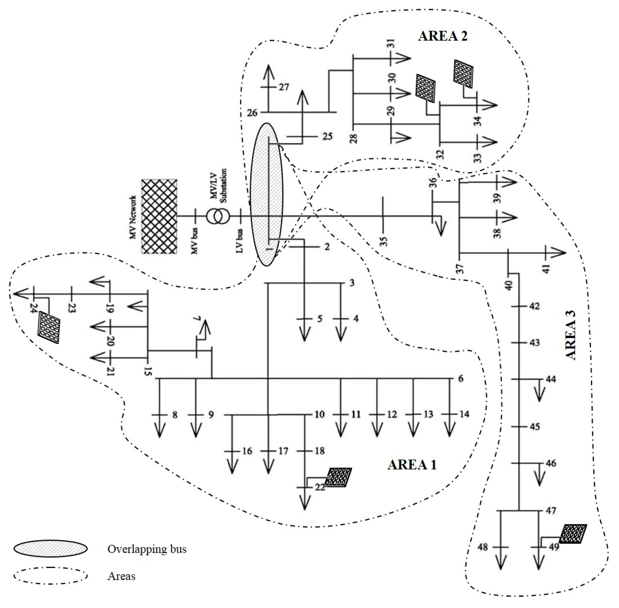
The proposed methodology was tested on the real three-phase distribution network shown in Figure 3, whose data are available in [29]. It consists of an LV distribution network (380 V) connected to an MV distribution system through a transformer substation (250 kVA). The short circuit power of the main network is 300 MVA. The primary substation, whose transformer tap is fixed at 1.05 p.u., is assumed to be the slack bus.
As shown in Figure 3, the system under investigation consists of 34 loads on 49 total buses, with an active power of 345.5 kW. Reactive powers of loads were obtained considering load power factors equal to 0.9. For this study, five PV generators were assumed to be connected at the buses 22, 24, 32, 34, and 49. These generators are identical with a maximum rated power of 30 kWp.
All computer simulations were carried out using the software package Matlab/Simulink [30]. All per unit data are referred to a base of 250 kVA.
We performed four tests aimed at investigating the ability of the proposed controller to cover the worst conditions in the voltage regulation.
For all tests, we assumed to be the reference value for all control buses.
4.1. Test 1—High Loads and Low PV Generations
The aim of this test is to investigate the controller’s aptitude to cover the risk of under-voltages. For this reason, it was assumed that each PV system generates approximately 8% of its rated power and that all system loads are at their rated power values.
Starting from this operating condition the proposed controller was started. Assuming a threshold equal to 0.55, the network was decomposed into three areas as shown in Figure 3. Note that, the three areas share bus 1, which represents the overlapping node. Subsequently, a control bus was identified for each of the three areas as reported in Table 1.
For this network partitioning, in the last column we report the set of boundary nodes for each control area.
Once the voltage control areas have been identified, the proposed methodology was separately applied to each of them. For clarity purposes, since its implementation is the same for all areas, details are given only for Area 1.
Note that this area consists of one swing bus (bus 1), a control bus (bus 6), and two PV generators that are connected at buses 22 and 24. We assumed that these buses are equipped with electronic metering devices capable of continuously measuring and transmitting the required electric variables to the area controller. These data (i.e., active and reactive powers as well as voltages) were fed into the developed non-linear optimization algorithm, where they were processed to evaluate the optimal control laws that must be sent to the local controllers of the two PV inverters belonging to the given area. The non-linear optimization algorithm has the following steps:
Step (1) Initialization phase
This phase can be in turn subdivided into two sub-phases. One is to generate the set of control variables and, the second one is to set the initial value for each of them.
Note that, for the given area the control variables vector can be defined as follows:
where
- -
- is the 3-dimensional column vector of unknown voltage phases which can be defined as: .
- -
- is the -dimensional equivalent admittance matrix of the reduced network model, which can be expressed as:
- -
- is the 2-dimensional column vector of the reactive power outputs of PV systems which can be expressed as: .
Once the set of the control variables was evaluated, an initial value was assumed for each of them. In particular, for our simulations a flat condition equal to zero was assumed for the all control variables.
Step (2) Evaluate the objective function
In this phase, the objective function, , defined in (13) was evaluated. In doing this, the two indices and were determined. In particular, the fitting error can be evaluated as:
where and are the model outputs for the generic i-th node. As can be noted, these models are expressed in terms of nodal admittance matrix and state vector (i.e., magnitude and phase voltages) at the boundary nodes of the equivalent network. Thus, the derived equations correspond to the load-flow equations.
The second index is evaluated by means of the following equation:
where is the measured voltage magnitude at the control bus, and is the desired voltage magnitude at the control bus.
Step (3) Sensitivities evaluation
Evaluate the sensitivities of the error function with regard to the control variables by means of Equations (21)–(26).
Step (4) Control variables evaluation
By means of Equation (20) the updating laws of the control variables were evaluated.
For clarity purposes only, the steady-state value of the identified admittance matrix was reported.
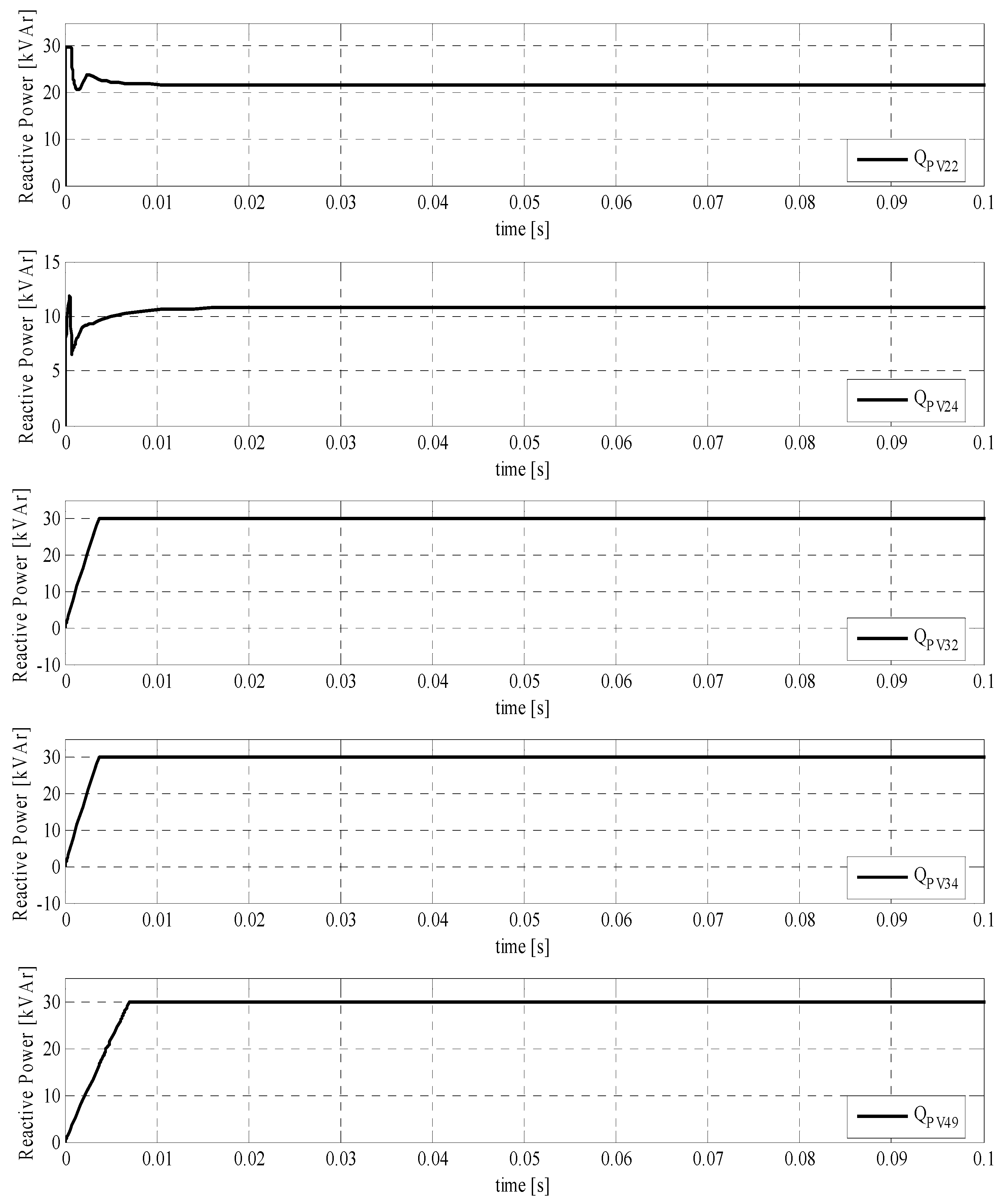
Figure 4 shows the time domain behavior of the reactive powers identified by all area controllers whereas Figure 5 reports the corresponding impact on their control buses.
As can be noted, all area controllers rapidly forced their own PV inverters to provide the reactive power needed to bring the control nodes voltages at their reference values. Note that, each generator is “called” to furnish a different amount of reactive power, depending on their individual contributions to the objective function. In particular, PV generators belonging to Areas 2 and 3 reached their upper limits, whereas those belonging to the Area 1 still have reactive margins.
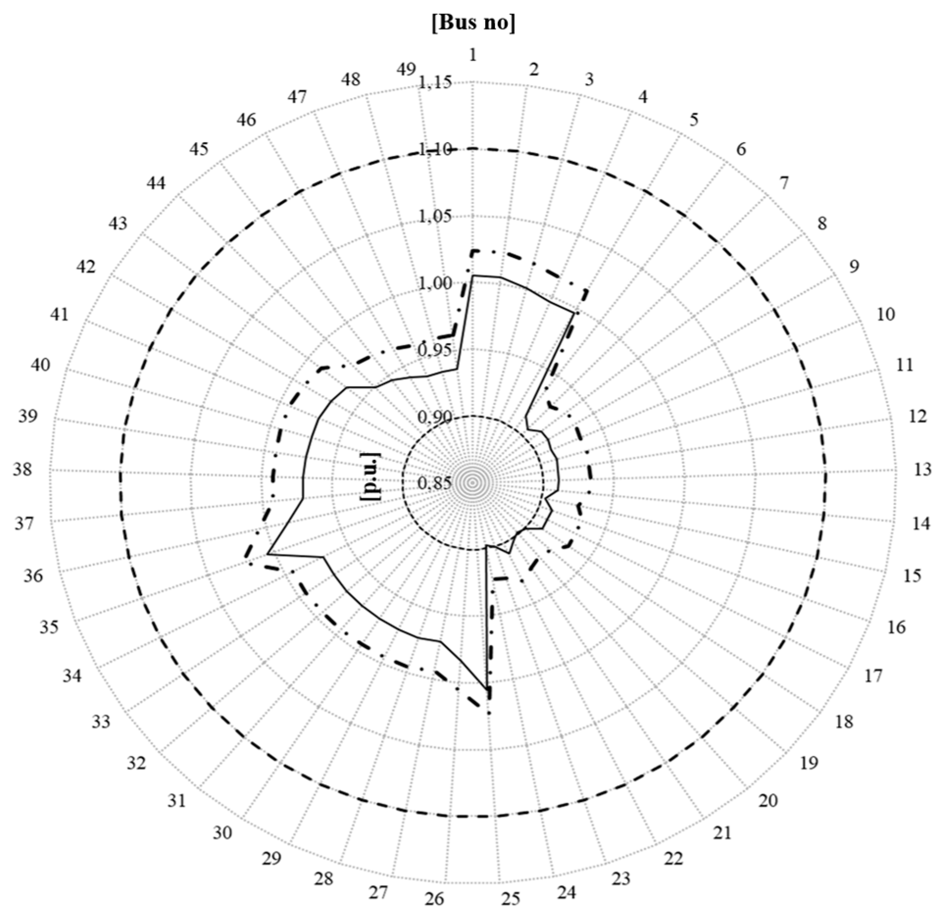
The optimization of the control buses voltages inevitably reverberated on the voltage profile of the unreduced network. In order to evaluate this indirect effect, we performed an a posteriori load-flow analysis on the overall system. Figure 6 reports the resulting voltage profile. For comparison purposes, in the same figure, we reported also the voltage profile evaluated on the unreduced network when no control action is applied. The same figure, reports also the voltage limits, i.e., ± 10% of its rated value, according to the standard EN 50160 [31].
As can be noted, considerable voltage drop occurs across the entire network when the reactive power control is turned off. The worst voltages are on those buses that are located far away from the primary substation. In fact, as can be seen from Figure 6, these nodes exhibited voltages closer to their lower limits. In particular, bus 24 experienced violation of the voltage lower limit (0.9 p.u.).
In order to investigate on the effectiveness of the proposed controller, we replicated the same test by applying the centralized controller developed in [16]. To compare the obtained results with those obtained from the proposed decentralized method, the following performance index was adopted:
where is the 49-dimensional column vector of nodal voltage magnitude and is the 49-dimensional column vector of the assumed nodal reference magnitudes.
Note that, the proposed performance index is an estimate of the voltage profile improvement. In fact, it measures how far the nodal voltage profile is from the assumed reference value.
Table 2 summarizes the results obtained by assuming for all network buses a reference value equal to one p.u.
As can be seen, the proposed method is slightly less performant than the centralized one, even if good results are provided. In fact, Table 2 indicates that the proposed controller improved the network voltage profile by about 22% over the non-optimized condition. As can be seen, this value is lower only by about 7% compared to the centralized optimization condition, confirming thus the effectiveness of the proposed method.
4.2. Test 2—Impact of the Noise on the Voltage Control
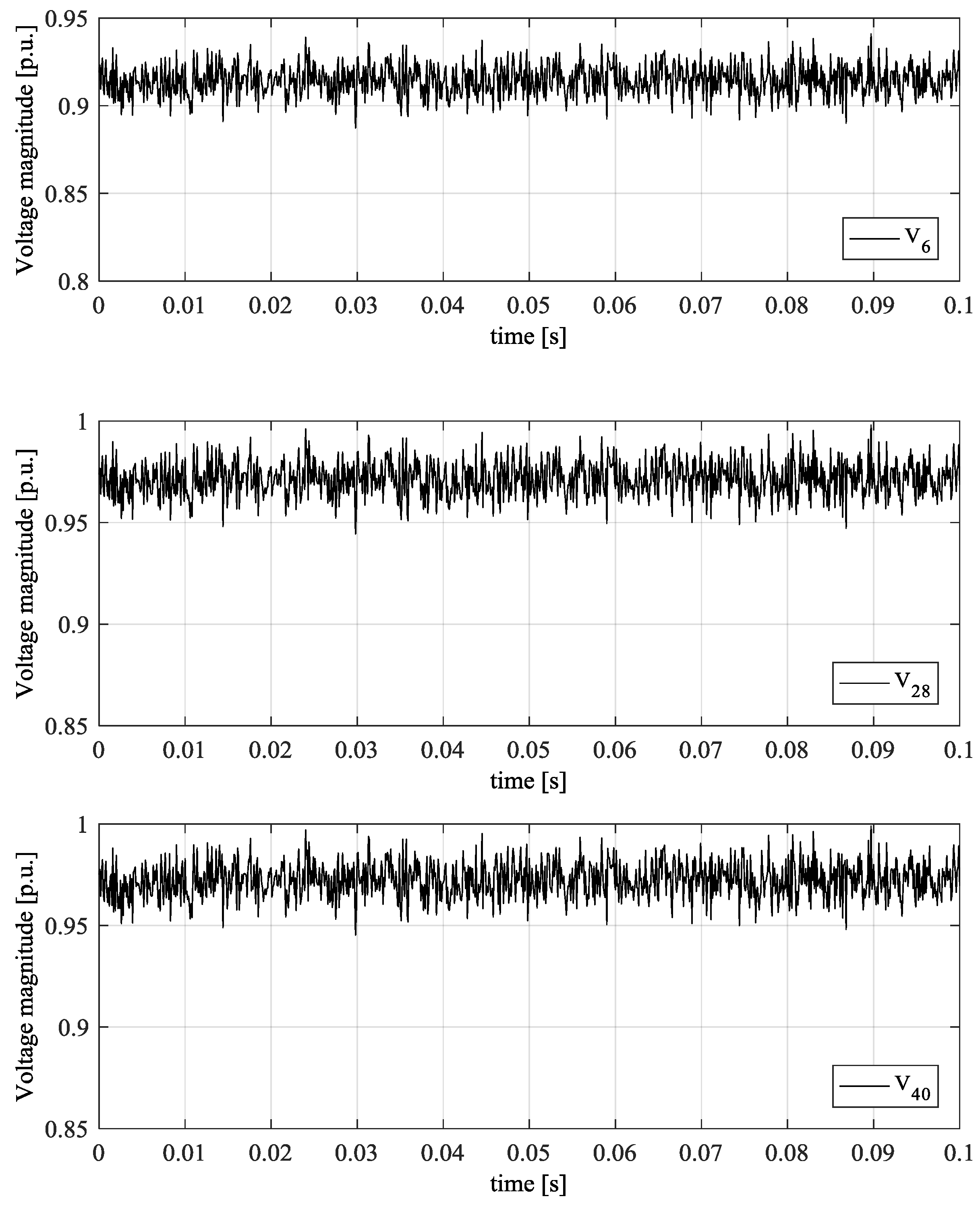
The aim of this test was to investigate the effects that incorrect measurement has on the controller’s performances. For this purpose, we replicated the above test by adding a white noise with a standard deviation equal to 0.01 p.u. on the measurements coming from the field. For clarity purposes, in Figure 7 we reported only the voltage magnitudes of the three control buses: 6, 28, and 40.
Figure 8 reports the time domain behavior of the identified reactive power control laws. As can be seen, the resulting control laws are quite uncorrupted by noise and, consequently reached the same steady-state values obtained in the previous test case. This is mainly due to the filtering action of the integrator in the feedback loop of the developed algorithm.
4.3. Test 3—Low Loads and High PV Generations
The aim of this test was to investigate on the controller’s ability to recover over-voltages occurring on the system.
In this test case, loads were considered at 27% and PV generators at 67% of their respectively rated values. Starting from this operating condition, we simultaneously turned on all area controllers. Figure 9 reports the derived reactive power control laws. For clarity purposes, we avoided including in this figure the time domain behaviors of the reactive power outputs of the two PV-inverters belonging to the Area 2, because they are similar to those enclosed in Area 1.
As can be noted, the PV inverters connected at buses 22, 24, 32, and 34, were forced to inject their minimum allowable reactive power, equal to −22.25 kVAr, whereas the PV inverter at bus 40 was forced to provide a reactive power equal to −20 kVAr.
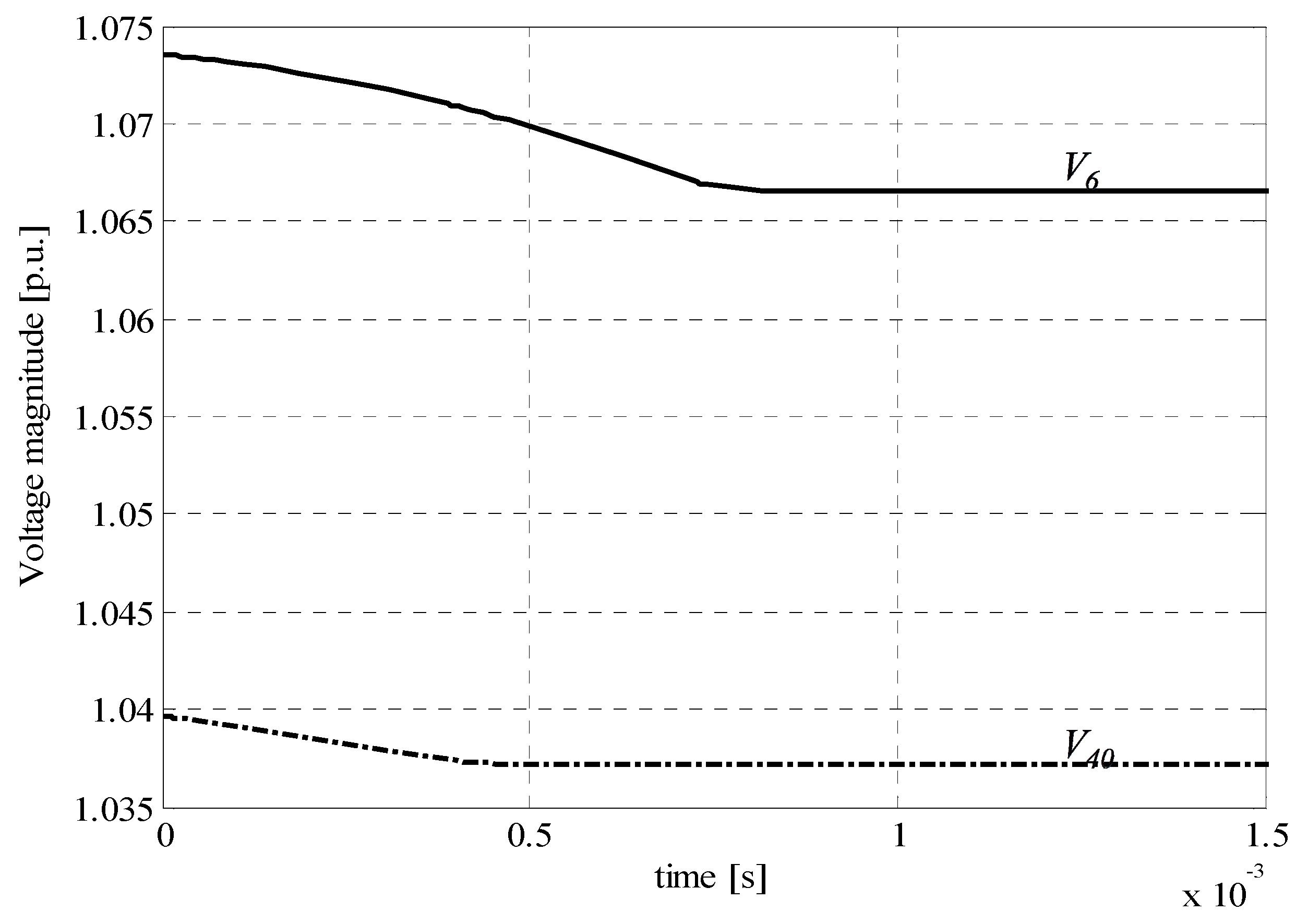
With these control actions, the voltages at control buses belonging to the Area 1 and 3 were forced to be as close as possible to their reference values as shown in Figure 10.
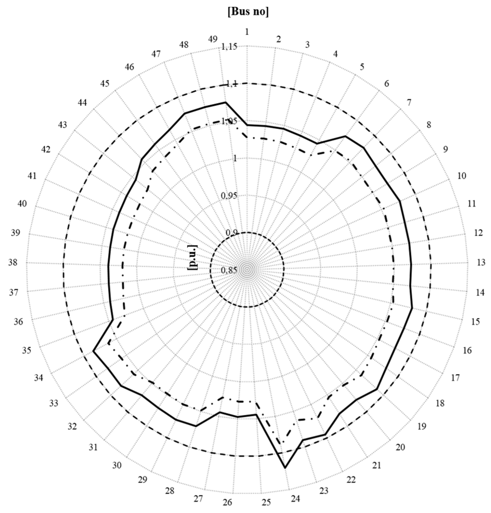
In order to evaluate the effectiveness of the developed control strategy, we suddenly turned off the controller. In Figure 11, we reported the network voltage profile evaluated with and without voltage control actions. The obtained results demonstrated that the evaluated control actions are able to bring the network voltage profile within the limits.
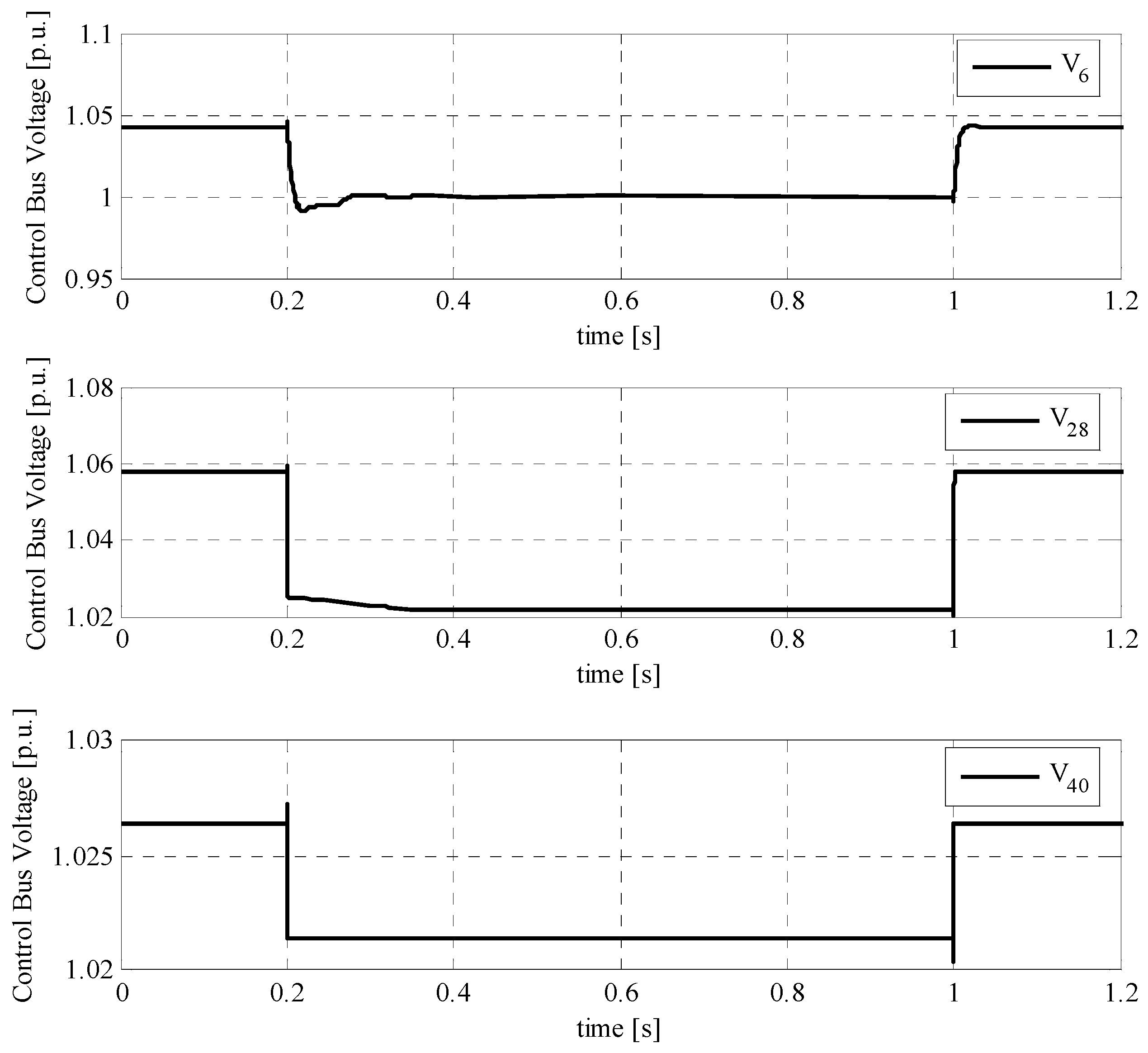
4.4. Test 4—Transient Event
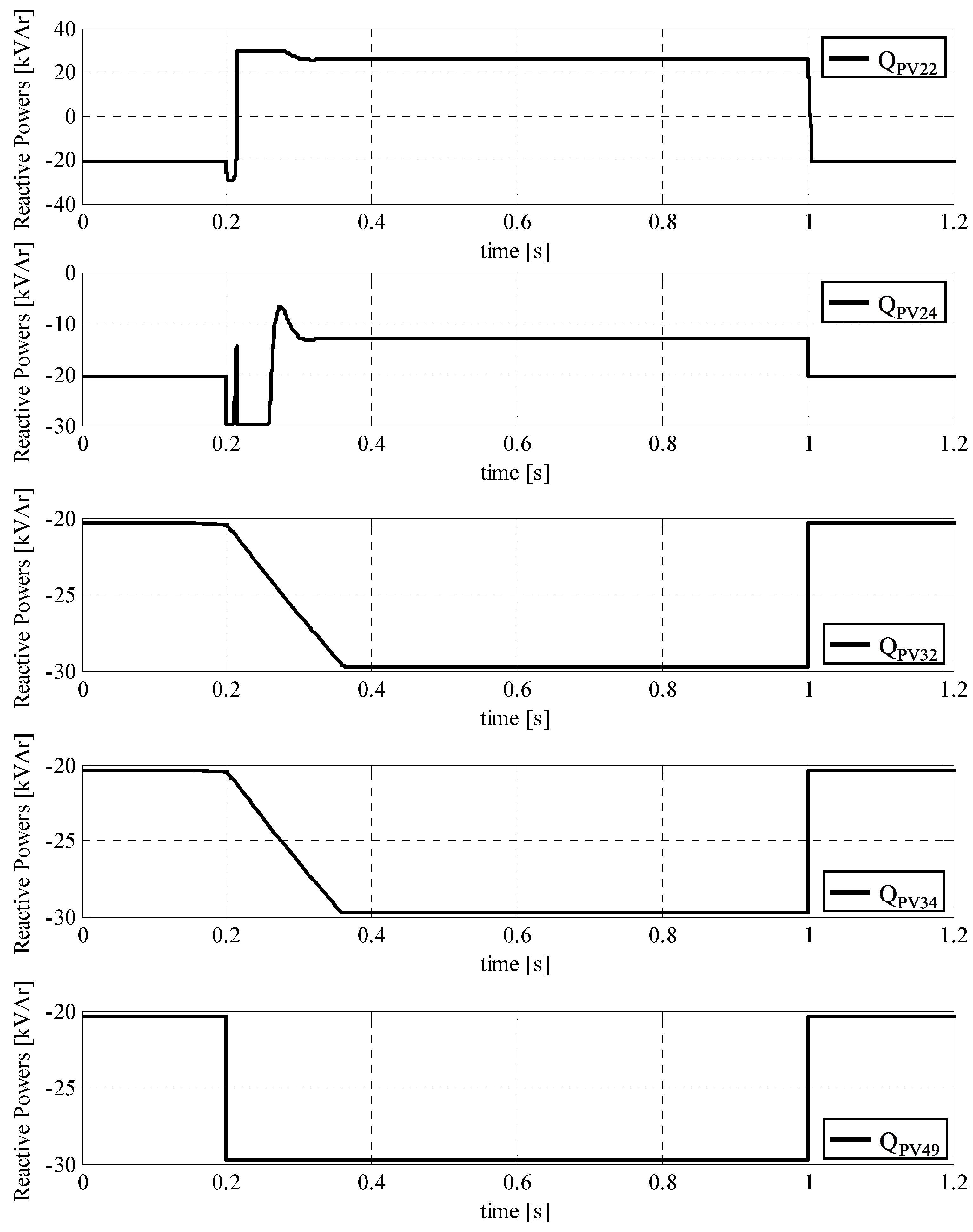
Starting from the previous optimized condition, a sudden change in PV generation was assumed. This transient event was simulated by reducing the active power produced by all PV plants from the value of 67% to the value of 8% at t = 0.2 s and then by returning to the pre-disturbance value at t = 1 s.
Figure 12 and Figure 13 report the time domain behaviors of the nodal voltages at the three selected control buses and of the control laws.
As can be noted, in the first stage of the transient the given disturbance implies a rapid rise in the control buses voltages. In response to this, the three decoupled algorithms rapidly forced their PV generators to absorb a large amount of reactive power. In the new steady-state condition, the PV inverters belonging to the Area 2 and 3 (i.e., 32, 34, and 49) reduced their reactive power injections to the value of −29.9 kVAr which is the minimum allowable reactive power. In fact, in this test case, since the active power provided by PV generators is equal to 2.4 kW (8%) the reactive power can range in the interval [−29.9, 29.9] kVAr.
At the same time, the algorithm acting on Area 1 forced the PV inverter connected at bus 24 to reduce its injection at a value of −29.9 kVAr, whereas the reactive power at bus 22 completely reversed to the value of 20.38 kVAr.
When the disturbance disappears, the pre-disturbance equilibrium point was restored.
5. Discussion
Test results showed the ability of the proposed controller to maintain a good voltage profile across the entire distribution network.
In all of the examined cases, it was observed that when the proposed controller was turned on, no problem arose in the voltage profile since all nodal voltages were kept within their limits (± 10% of the nominal voltage value).
In order to investigate the ability of the proposed controller to work well in many practical applications, we stressed the algorithm by considering those operating conditions, which can give rise to voltage deviations difficult for it to handle. This analysis was performed through two tests that were specifically designed to cause undervoltage and overvoltage problems, respectively. Simulation results demonstrated the effectiveness of the proposed methodology and its ability to address both undervoltage and overvoltage problems, thus reducing the risk of the violation of the voltage limits.
Moreover, since in practical cases the field measurements are usually corrupted by noise, we performed another test in which a white noise was added to the measurements. Results revealed the self-filtering characteristic of the proposed controller due to the presence of the integrator in the algorithm. Thanks to this feature, the noise-corrupted measures do not represent a problem for the correct evaluation of the optimal control laws needed for the optimization of the network voltage profile.
A further simulation was carried out by simulating a sudden reduction of the active power generated by all PV plants. The obtained results demonstrated the controller’s ability to promptly react at any change in the system operating condition, confirming its application in the on-line environment.
Furthermore, we compared the results obtained from the proposed controller with those obtained from a centralized one. The comparison showed that the proposed controller provides solutions comparable with the centralized one, thus confirming its effectiveness and justifying its adoption.
6. Conclusions
In this paper, a multi-area voltage control scheme adopting the reactive power control capability of Distributed Generation (DG) units as reactive power providers was developed.
The proposed controller assumes that a structural decomposition is a priori performed to identify areas composing the distribution system. Once the control areas are identified, one or more control buses are selected for each of them and then a reduced equivalent model for each area can be obtained. An optimization problem of being able to evaluate an equivalent reduced network and to optimize the voltage magnitude at the control buses by controlling reactive powers at DG units was derived. The solution of this problem was obtained by adopting an algorithm operating in the continuous time domain based on a fast artificial dynamic system involving the Lyapunov theory.
An actual distribution network was used for testing the proposed methodology under several operating conditions, demonstrating that the suggested controller is able to optimize the system voltage profile in real time.
Author Contributions
Alessia Cagnano and Enrico De Tuglie conceived this study and designed the simulations. Alessia Cagnano performed the simulation tests. Alessia Cagnano and Enrico De Tuglie analyzed the test results and wrote the manuscript. Marco Bronzini contributed in writing the manuscript. All authors have read and approved the final manuscript.
Conflicts of Interest
The authors declare no conflict of interest. The founding sponsors had no role in the design of the study; in the collection, analyses, or interpretation of data; in the writing of the manuscript, and in the decision to publish the results.
References
- Vita, V.; Alimardan, T.; Ekonomou, L. The impact of distributed generation in the distribution networks’ voltage profile and energy losses. In Proceedings of the 9th IEEE European Modelling Symposium on Mathematical Modelling and Computer Simulation, Madrid, Spain, 6–8 October 2015; pp. 260–265. [Google Scholar]
- Ch, Y.; Goswami, S.K.; Chatterjee, D. Effect of network reconfiguration on power quality of distribution system. Int. J. Electr. Power Energy Syst. 2016, 83, 87–95. [Google Scholar] [CrossRef]
- Vita, V. Development of a decision-making algorithm for the optimum size and placement of distributed generation units in distribution networks. Energies 2017, 10, 1433. [Google Scholar] [CrossRef]
- Gopiya-Naik, S.; Khatod, D.K.; Sharma, M.P. Optimal allocation of distributed generation in distribution system for loss reduction. In Proceedings of the IACSIT Coimbatore Conferences, Coimbatore, India, 18–19 February 2012; Volume 28, pp. 42–46. [Google Scholar]
- Kaur, N.; Jain, S.K. Multi-Objective Optimization Approach for Placement of Multiple DGs for Voltage Sensitive Loads. Energies 2017, 10, 1733. [Google Scholar] [CrossRef]
- Kayal, P.; Chanda, C.K. Placement of Wind and Solar Based DGs in Distribution System for Power Loss minimization and voltage stability improvement. Int. J. Electr. Power Energy Syst. 2013, 53, 795–809. [Google Scholar] [CrossRef]
- Bruno, S.; Dassisti, M.; la Scala, M.; Chimienti, M.; Stigliano, G.; Palmisani, E. Managing Networked Hybrid-Energy Systems: A Predictive Dispatch Approach. In Proceedings of the IFAC, Cape Town, South Africa, 24–29 August 2014; Volume 47, pp. 2394–2399. [Google Scholar]
- Eremia, M.; Tawfeeq, A.B.L. Reactive power optimization based on genetic algorithm with new technique of mutation. In Proceedings of the 2014 International Symposium on Fundamentals of Electrical Engineering (ISFEE), Bucharest, Romania, 28–29 November 2014; pp. 1–5. [Google Scholar]
- Cagnano, A.; Torelli, F.; Alfonzetti, F.; de Tuglie, E. Can PV plants provide a reactive power ancillary service? A treat offered by an on-line controller. Renew. Energy 2011, 36, 1047–1052. [Google Scholar] [CrossRef]
- De Tuglie, A.C.E.; Liserre, M.; Mastromauro, R.A. Online optimal reactive power control strategy of PV inverters. IEEE Trans. Ind. Electron. 2011, 58, 4549–4558. [Google Scholar]
- Bolognani, S.; Zampieri, S. A distributed control strategy for reactive power compensation in smart microgrids. IEEE Trans. Autom. Control 2013, 58, 2818–2833. [Google Scholar] [CrossRef]
- Ahn, C.; Peng, H. Decentralized voltage control to minimize distribution power loss of microgrids. IEEE Trans. Smart Grid 2013, 4, 1297–1304. [Google Scholar] [CrossRef]
- Delfino, F.; Denegri, G.B.; Invernizzi, M.; Procopio, R. An Integrated Active and Reactive Power Control Scheme for Grid-Connected Photovoltaic Production Systems. In Proceedings of the IEEE 39th Power Electronics Specialists Conference PESC, Rhodes, Greece, 15–19 June 2008. [Google Scholar]
- Cagnano, A.; de Tuglie, E.; Dicorato, M.; Forte, G.; Trovato, M. PV plants for voltage regulation in distribution networks. In Proceedings of the 2012 47th International Universities Power Engineering Conference (UPEC), London, UK, 4–7 September 2012; pp. 1–5. [Google Scholar]
- Malekpour, A.R.; Pahwa, A. Reactive Power and Voltage Control in Distribution Systems with Photovoltaic Generation. In Proceedings of the North American Power Symposium (NAPS) 2012, Champaign, IL, USA, 9–11 September 2012. [Google Scholar]
- Cagnano, A.; de Tuglie, E. Centralized voltage control for distribution networks with embedded PV systems. Renew. Energy 2015, 76, 173–185. [Google Scholar] [CrossRef]
- Bronzini, M.; Bruno, S.; la Scala, M.; Sbrizzai, R. Coordination of active and reactive distributed resources in a smart grid. In Proceedings of the IEEE Trondheim PowerTech, Trondheim, Norway, 19–23 June 2011; pp. 1–7. [Google Scholar]
- Aristidou, P.; Olivier, F.; Hervas, M.E.; Ernst, D.; van Cutsem, T. Distributed Model-Free control of photovoltaic units for mitigating overvoltages in low voltage networks. In Proceedings of the CIRED 2014 Workshop “Challenges of implementing Active Distribution System Management”, Rome, Italy, 11–12 June 2014. [Google Scholar]
- Carvalho, P.M.S.; Correia, P.F.; Ferreira, L.A.F.M. Distributed reactive power generation control for voltage rise mitigation in distribution networks. IEEE Trans. Power Syst. 2008, 23, 766–772. [Google Scholar] [CrossRef]
- Fakham, H.; Ahmidi, A.; Colas, F.; Guillaud, X. Multi-agent system for distributed voltage regulation of wind generators connected to distribution network. In Proceedings of the 2010 IEEE PES Innovative Smart Grid Technologies Conference Europe (ISGT Europe), Gothenberg, Sweden, 11–13 October 2010; pp. 1–6. [Google Scholar]
- Fallahzadeh-Abarghouei, H.; Nayeripour, M.; Hasanvand, S.; Waffenschmidt, E. Online hierarchical and distributed method for voltage control in distribution smart grids. IET Gener. Transm. Distrib. 2017, 11, 1223–1232. [Google Scholar] [CrossRef]
- Saravanakathir, B.; Sasiraja, R.M. Optimal Coordinated Voltage Control Method for Distribution Network in Presence of Distributed Generators. Int. J. Eng. Sci. 2017, 7, 12117–12122. [Google Scholar]
- Bahramipanah, M.; Cherkaoui, R.; Paolone, M. Decentralized voltage control of clustered active distribution network by means of energy storage systems. Electr. Power Syst. Res. 2016, 136, 370–382. [Google Scholar] [CrossRef]
- Nayeripour, M.; Fallahzadeh-Abarghouei, H.; Waffenschmidt, E.; Hasanvand, S. Coordinated online voltage management of distributed generation using network partitioning. Electr. Power Syst. Res. 2016, 141, 202–209. [Google Scholar] [CrossRef]
- Sun, H.; Guo, Q.; Zhang, B.; Wu, W.; Wang, B. An adaptive zone-division-based automatic voltage control system with applications in China. IEEE Trans. Power Syst. 2013, 28, 1816–1828. [Google Scholar] [CrossRef]
- Morattab, A.; Akhrif, O.; Saad, M. Decentralised coordinated secondary voltage control of multi-area power grids using model predictive control. IET Gener. Transm. Distrib. 2017, 11, 4546–4555. [Google Scholar] [CrossRef]
- De Tuglie, E.; Iannone, S.M.; Torelli, F. A coherency recognition based on structural decomposition procedure. IEEE Trans. Power Syst. 2008, 23, 555–563. [Google Scholar] [CrossRef]
- Milano, F. Power System Modelling and Scripting; Springer: Berlin, Germany, 2010. [Google Scholar]
- Passoni, S. Partecipazione dei Generatori al Controllo Della Tensione Sulla Rete BT. Available online: http://hdl.handle.net/10589/49301 (accessed on 15 June 2012).
- The Math Works. Matlab/Simulink User’s Guide; The Math Works: Natick, MA, USA, 2016. [Google Scholar]
- European Committee for Electrotechnical Standardization. EN 50160: Voltage Characteristics of Electricity Supplied by Public Distribution Systems; European Committee for Electrotechnical Standardization: Brussels Belgium, 1999. [Google Scholar]
Figure 1.
Block diagram of the proposed fitting error.
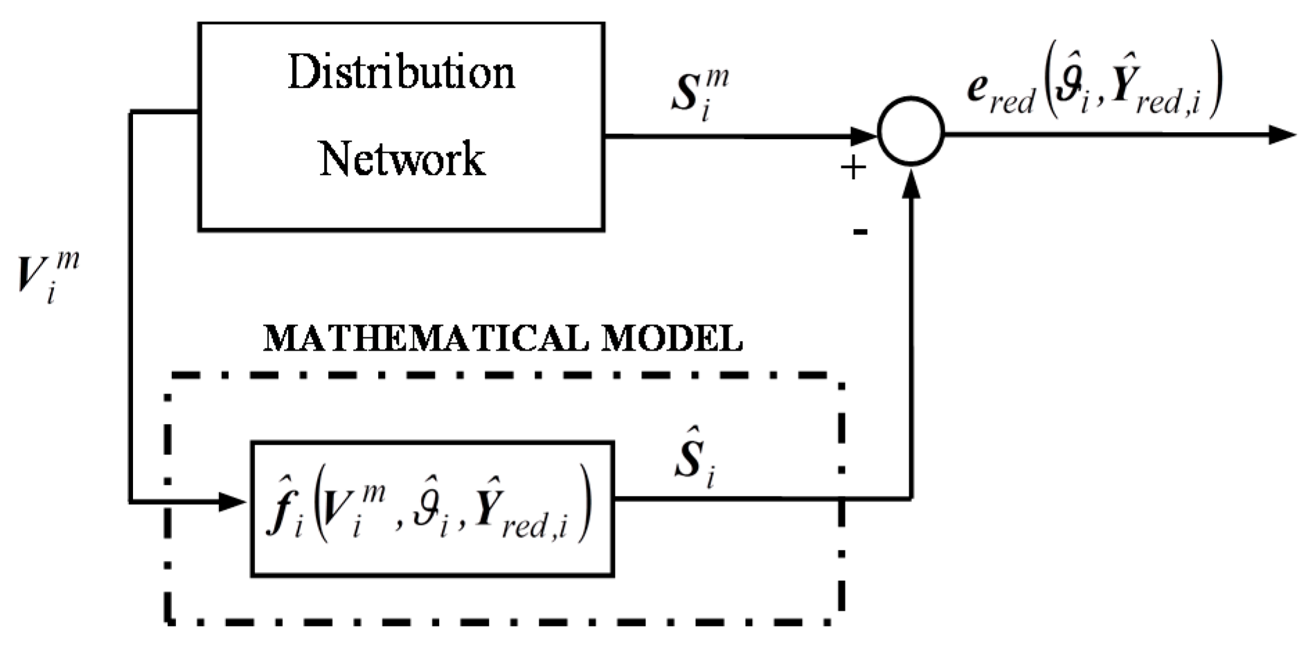
Figure 2.
Flow-chart of the proposed optimization algorithm.
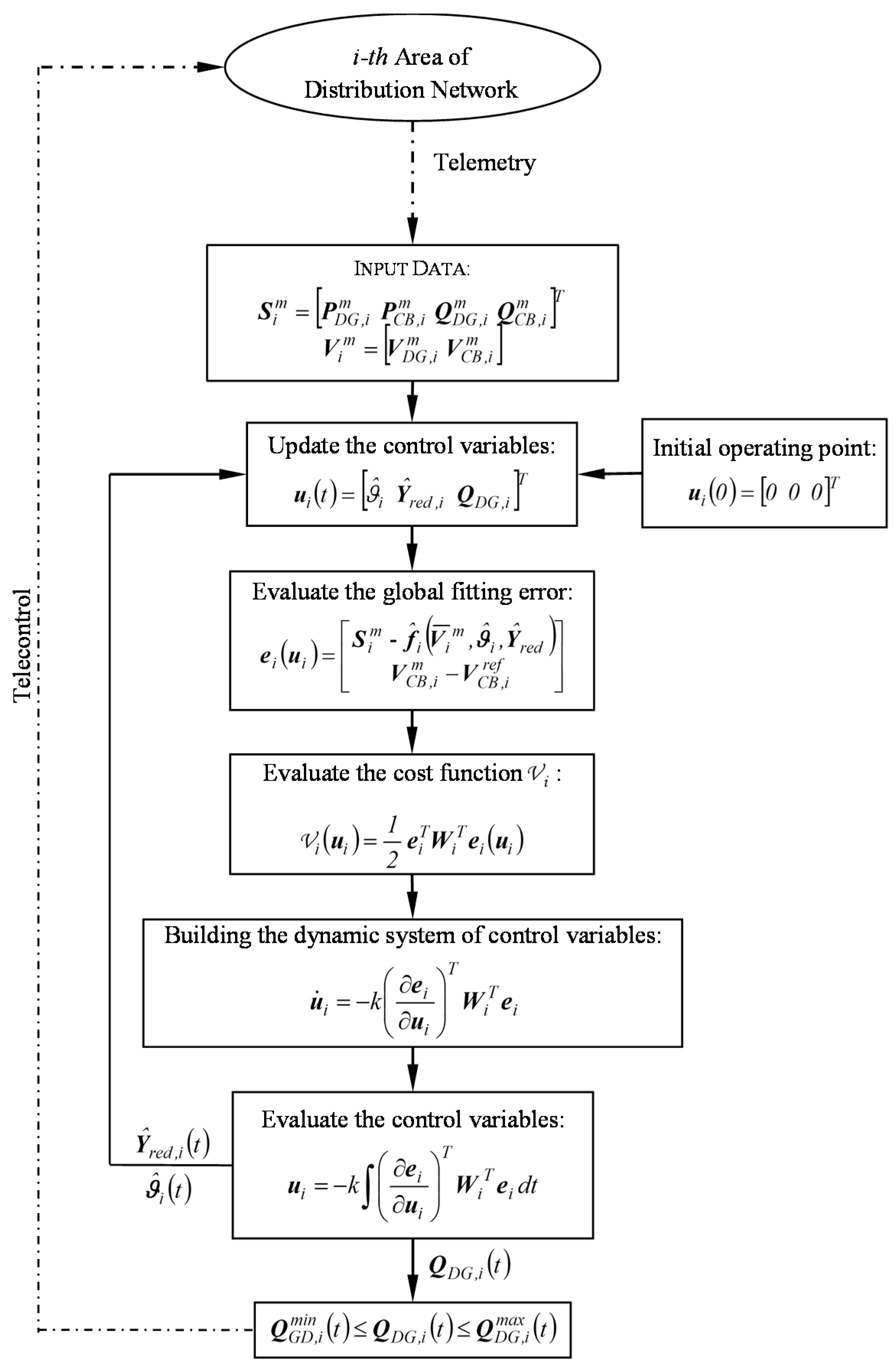
Figure 3.
The single line diagram of the test distribution network.

Figure 4.
Reactive power control laws at the PV-inverters.

Figure 5.
Time domain behavior of the voltage at the selected control buses.
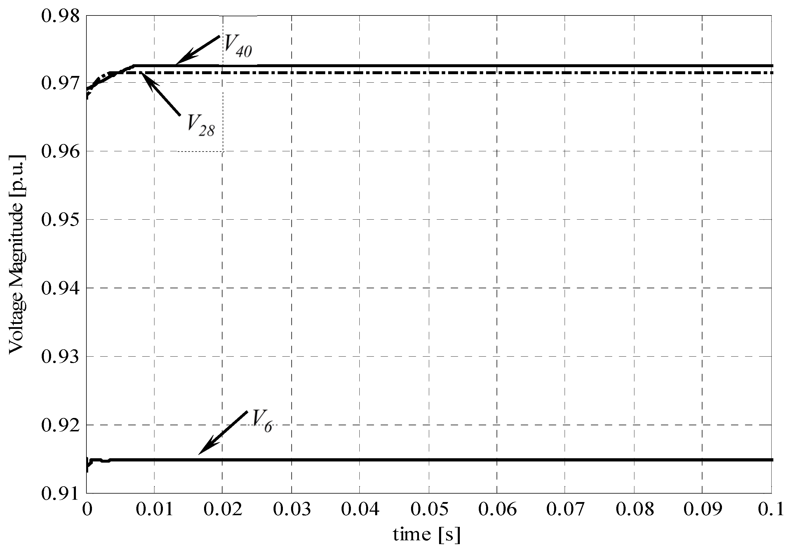
Figure 6.
Network voltage profile with (dotted-dashed line) and without (solid line) the voltage controllers. Dashed lines refer to voltage limits.
Figure 6.
Network voltage profile with (dotted-dashed line) and without (solid line) the voltage controllers. Dashed lines refer to voltage limits.

Figure 7.
The simulated voltage magnitudes on the three control buses: 6, 28, and 40.

Figure 8.
The estimated reactive power control laws at the PV-inverters.
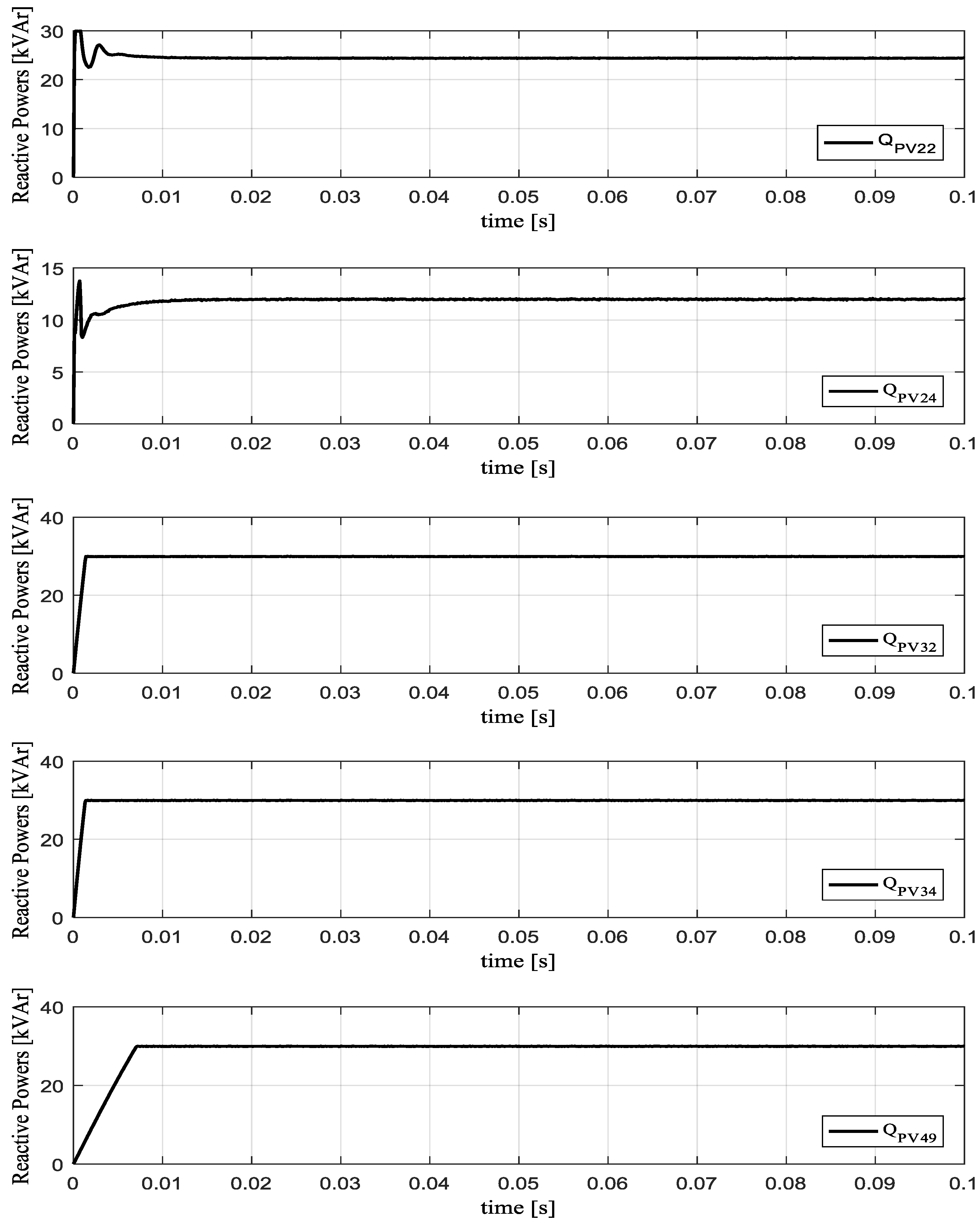
Figure 9.
Time domain behavior of reactive power outputs of the PV-inverters connected at the buses #22, 24, and 49.
Figure 9.
Time domain behavior of reactive power outputs of the PV-inverters connected at the buses #22, 24, and 49.
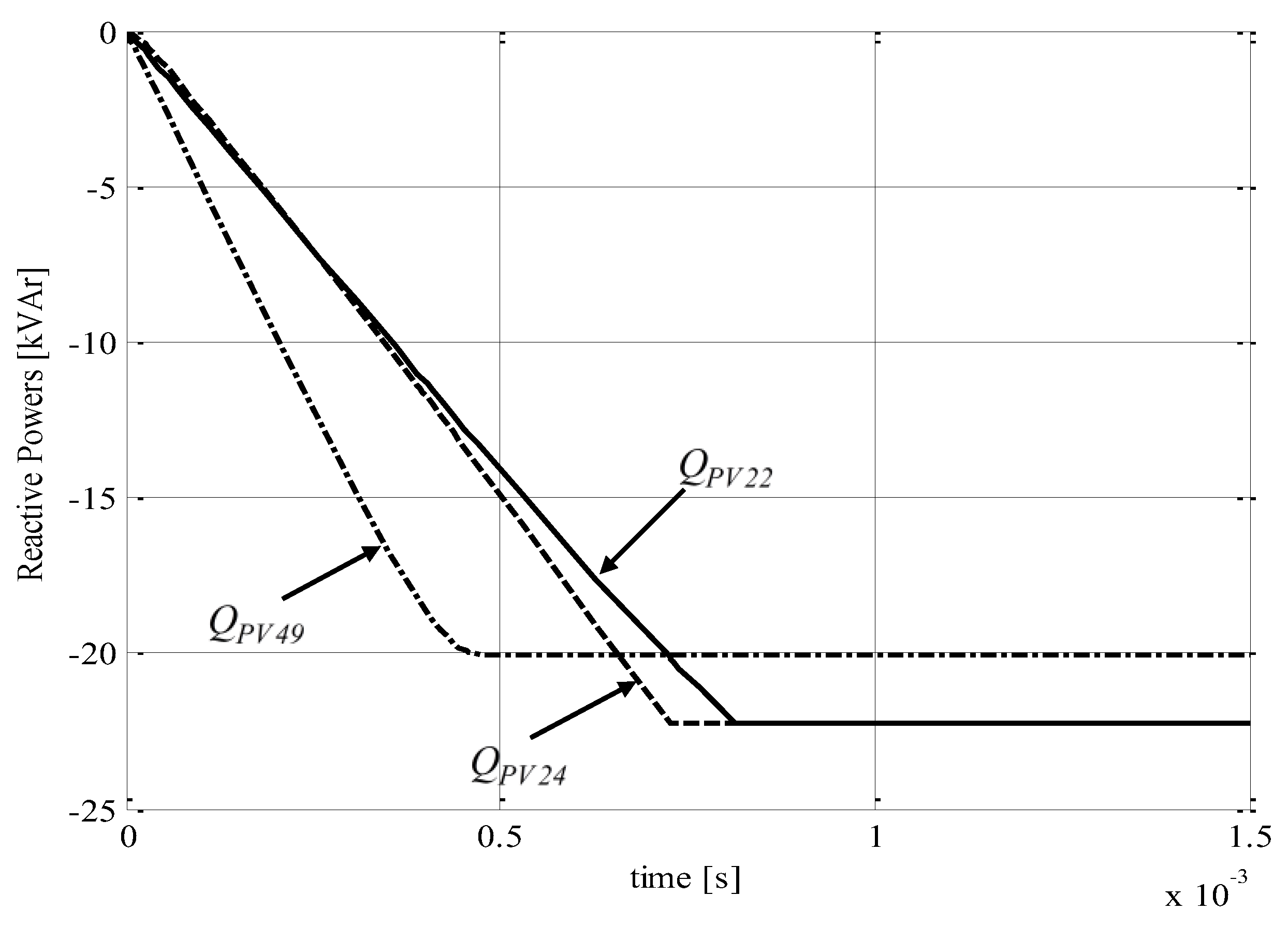
Figure 10.
Time domain behavior of the voltage at the control bus.

Figure 11.
Network voltage profile with (dotted-dashed line) and without (solid line) the voltage controllers. Dashed lines refer to voltage limits.
Figure 11.
Network voltage profile with (dotted-dashed line) and without (solid line) the voltage controllers. Dashed lines refer to voltage limits.

Figure 12.
Time domain behavior of the voltages at the selected control buses.

Figure 13.
Time domain behavior of reactive power outputs of the PV-inverters connected at buses #22, 24, 32, 34, and 49.
Figure 13.
Time domain behavior of reactive power outputs of the PV-inverters connected at buses #22, 24, 32, 34, and 49.

Table 1.
Voltage control areas and their associated control buses.
| Voltage Control Area | Sets of Buses Forming Voltage Control Areas | Control Buses | Boundary Area Nodes |
|---|---|---|---|
| Area 1 | 1–24 | 6 | 1, 6, 22, 24 |
| Area 2 | 1, 25–34 | 28 | 1, 28, 32, 34 |
| Area 3 | 1, 35–49 | 40 | 1, 40, 49 |
Table 2.
Comparison of the proposed method’s results with a centralized methodology.
| Methodology | Reactive Powers [kVAr] | Performance Index Ψ | ||||
|---|---|---|---|---|---|---|
| Bus 22 | Bus 24 | Bus 32 | Bus 34 | Bus 49 | ||
| No voltage control | 0 | 0 | 0 | 0 | 0 | 0.290 |
| Centralized controller | 15.00 | 10.96 | 30.00 | 30.00 | 30.00 | 0.210 |
| Multi-Area controller | 21.57 | 10.76 | 30.00 | 30.00 | 30.00 | 0.226 |
© 2018 by the authors. Licensee MDPI, Basel, Switzerland. This article is an open access article distributed under the terms and conditions of the Creative Commons Attribution (CC BY) license (http://creativecommons.org/licenses/by/4.0/).
Share and Cite
MDPI and ACS Style
Cagnano, A.; De Tuglie, E.; Bronzini, M. Multiarea Voltage Controller for Active Distribution Networks. Energies 2018, 11, 583. https://doi.org/10.3390/en11030583
AMA Style
Cagnano A, De Tuglie E, Bronzini M. Multiarea Voltage Controller for Active Distribution Networks. Energies. 2018; 11(3):583. https://doi.org/10.3390/en11030583
Chicago/Turabian StyleCagnano, Alessia, Enrico De Tuglie, and Marco Bronzini. 2018. "Multiarea Voltage Controller for Active Distribution Networks" Energies 11, no. 3: 583. https://doi.org/10.3390/en11030583
Note that from the first issue of 2016, this journal uses article numbers instead of page numbers. See further details here.