Energy Flexometer: Transactive Energy-Based Internet of Things Technology

 ,
, 
 ,
, 
Abstract
:1. Introduction
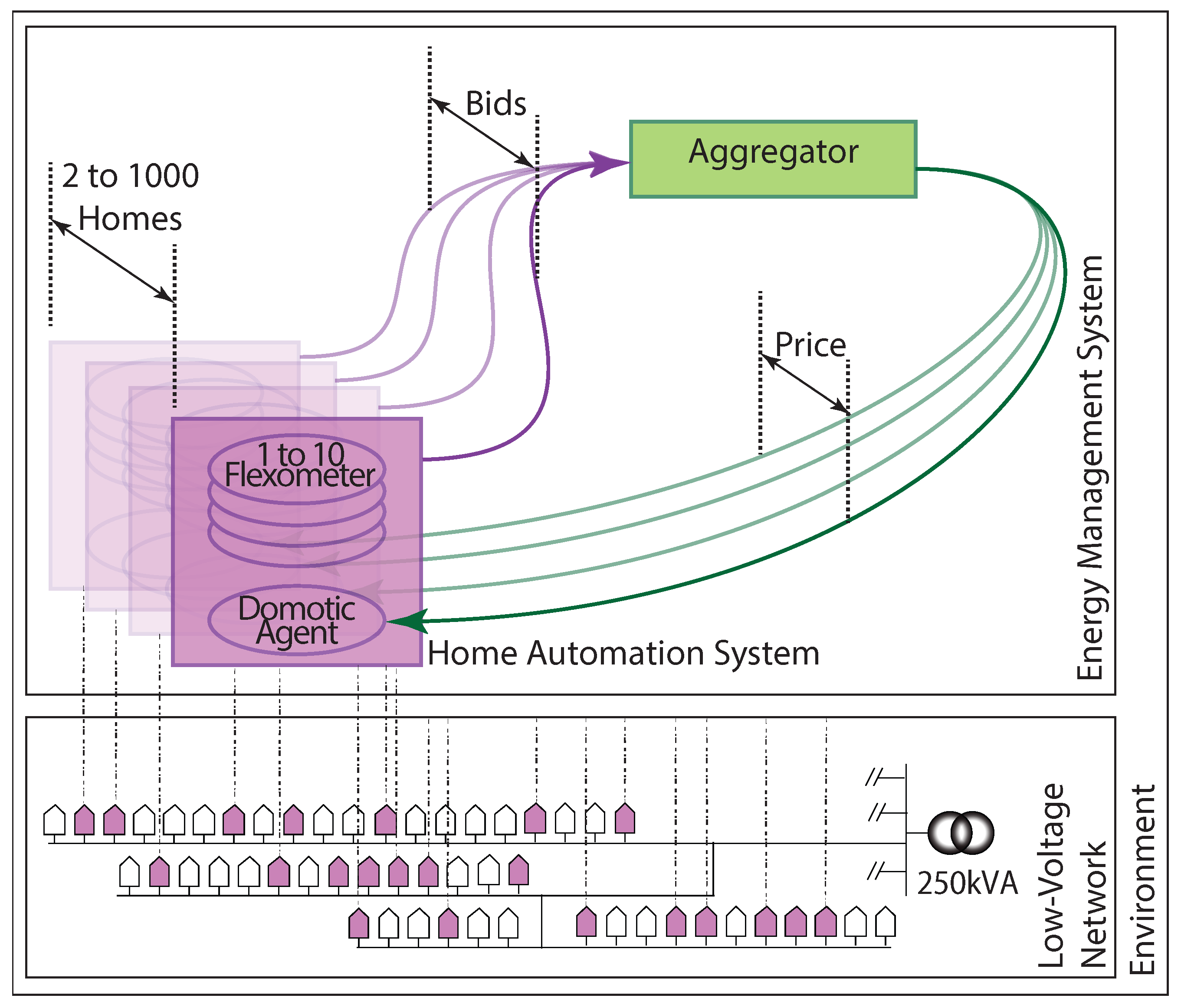
2. Design and Concept of Energy Flexometer
2.1. Concept
2.2. Design
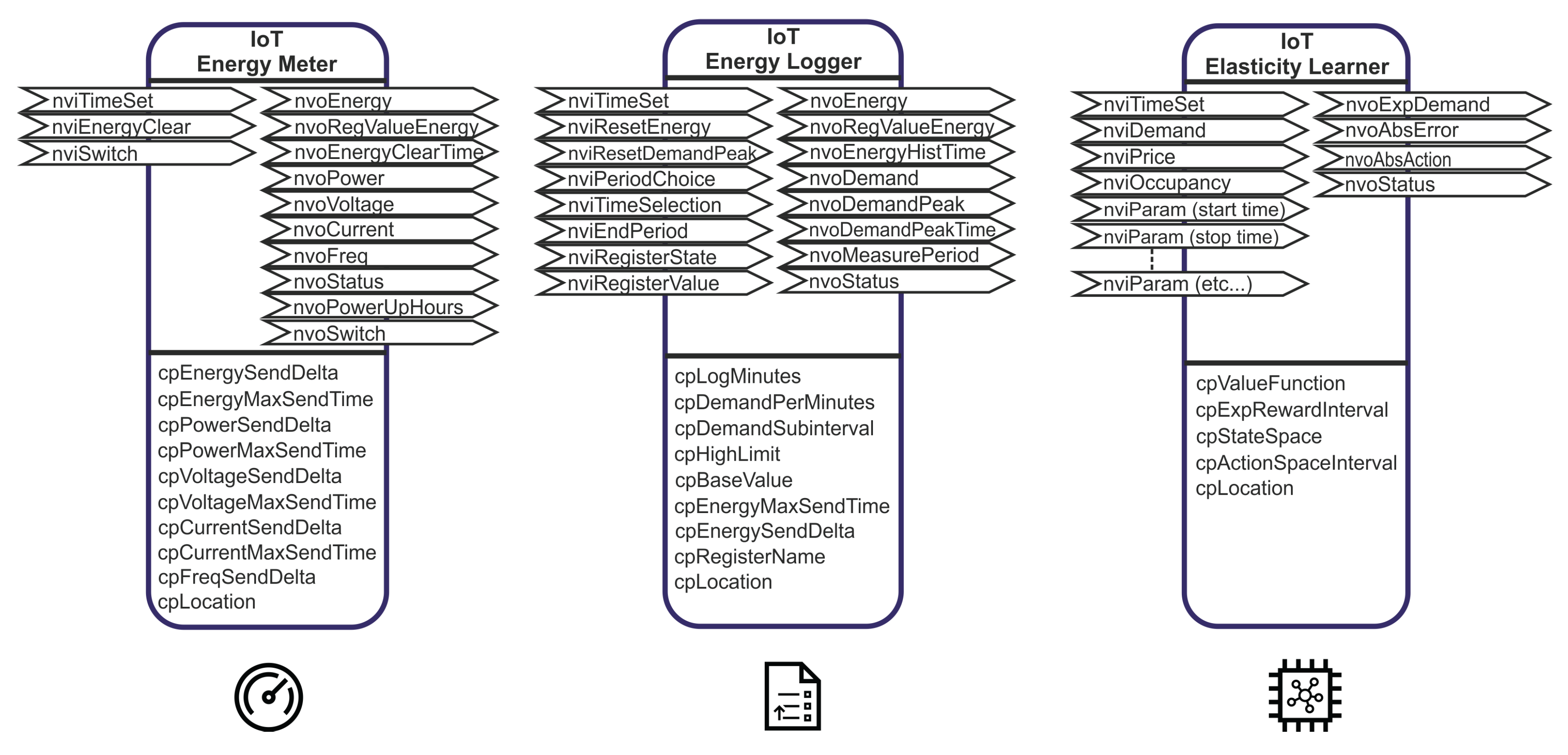
2.3. Energy Meter
2.4. Energy Logger
2.5. Energy Elasticity Learner
3. Demand Elasticity Estimation
3.1. State Space and Action Space
3.2. The Objective Function
3.3. Action Selection
| Algorithm 1: Demand Elasticity Estimation Algorithm. |
 |
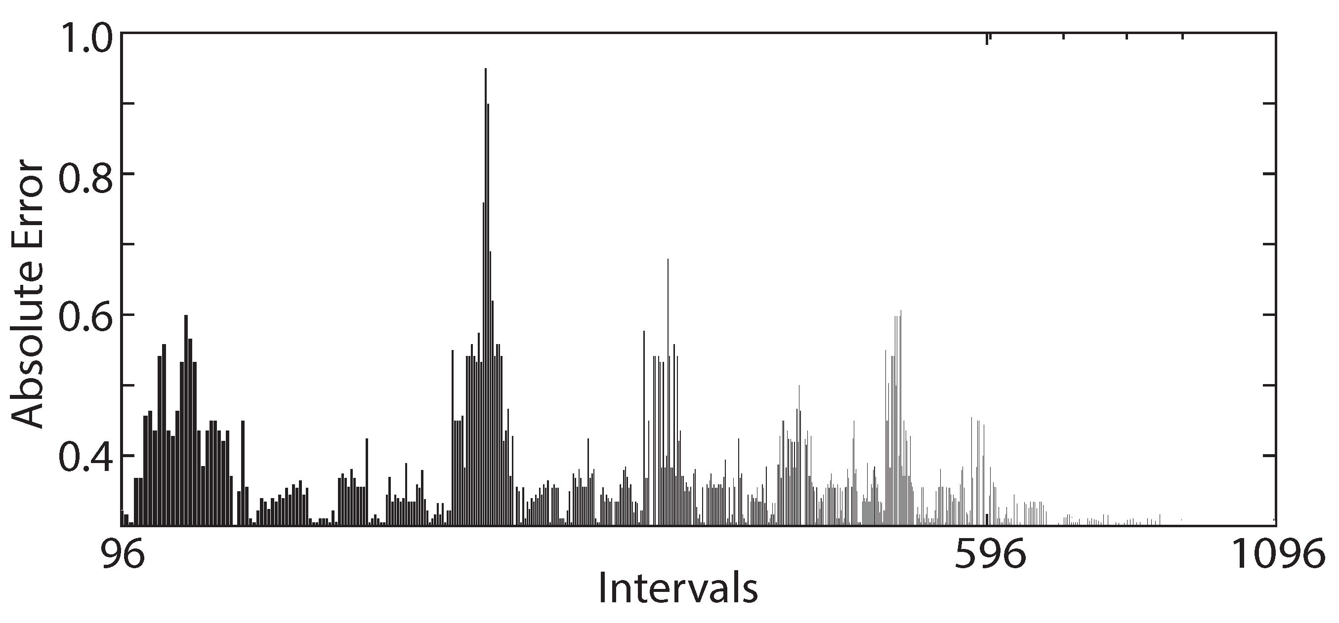
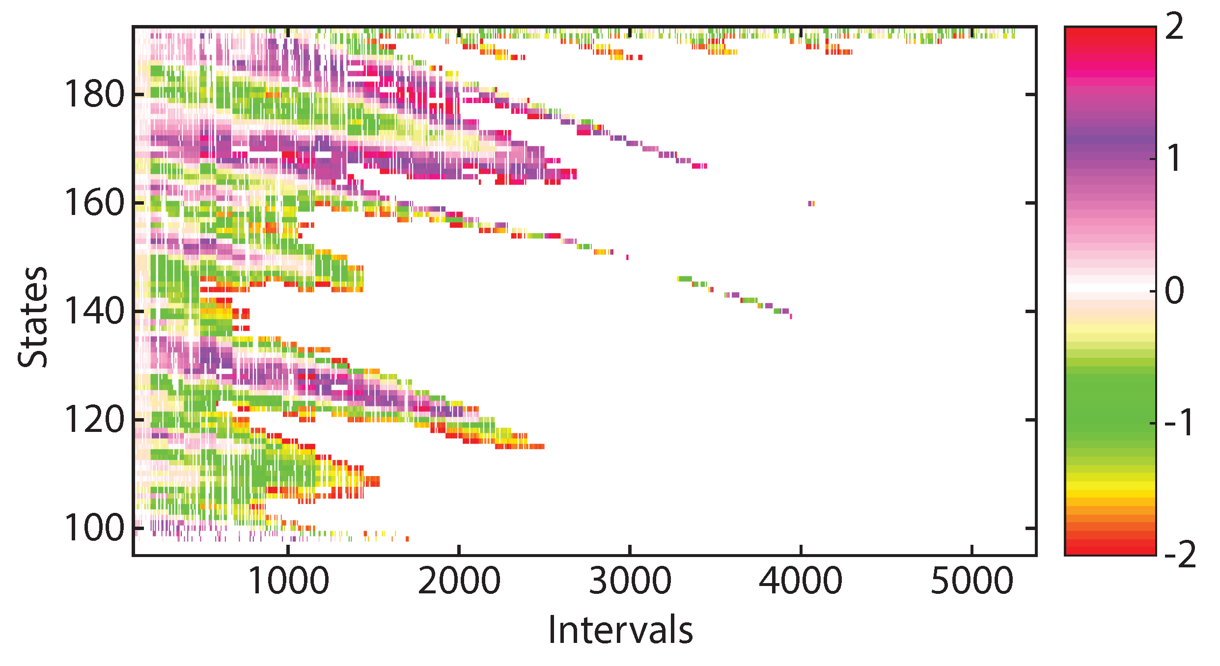
3.4. Simulation of Demand Elasticity by using the Algorithm
4. Physical Implementation
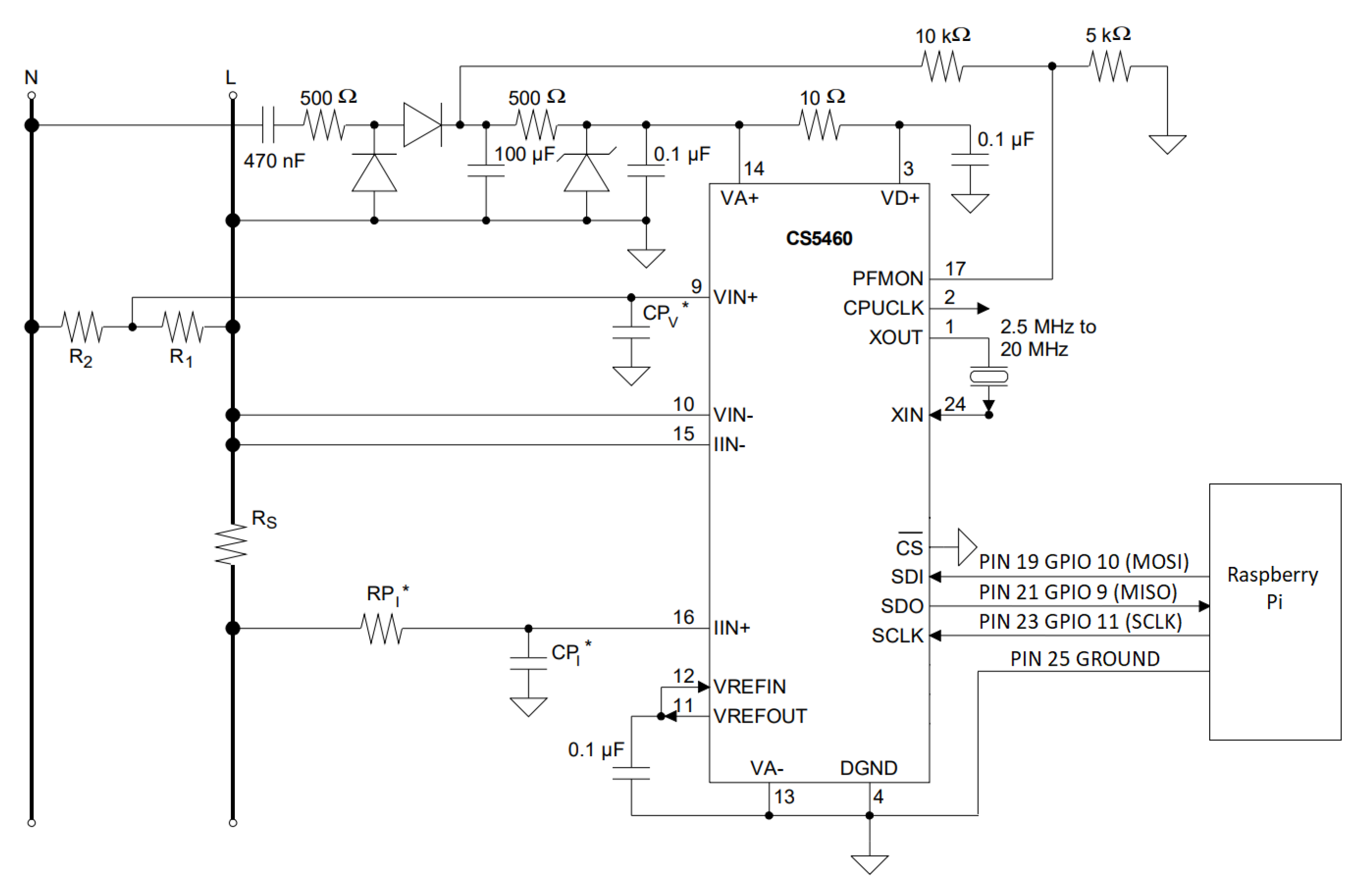
4.1. Measurement System Design
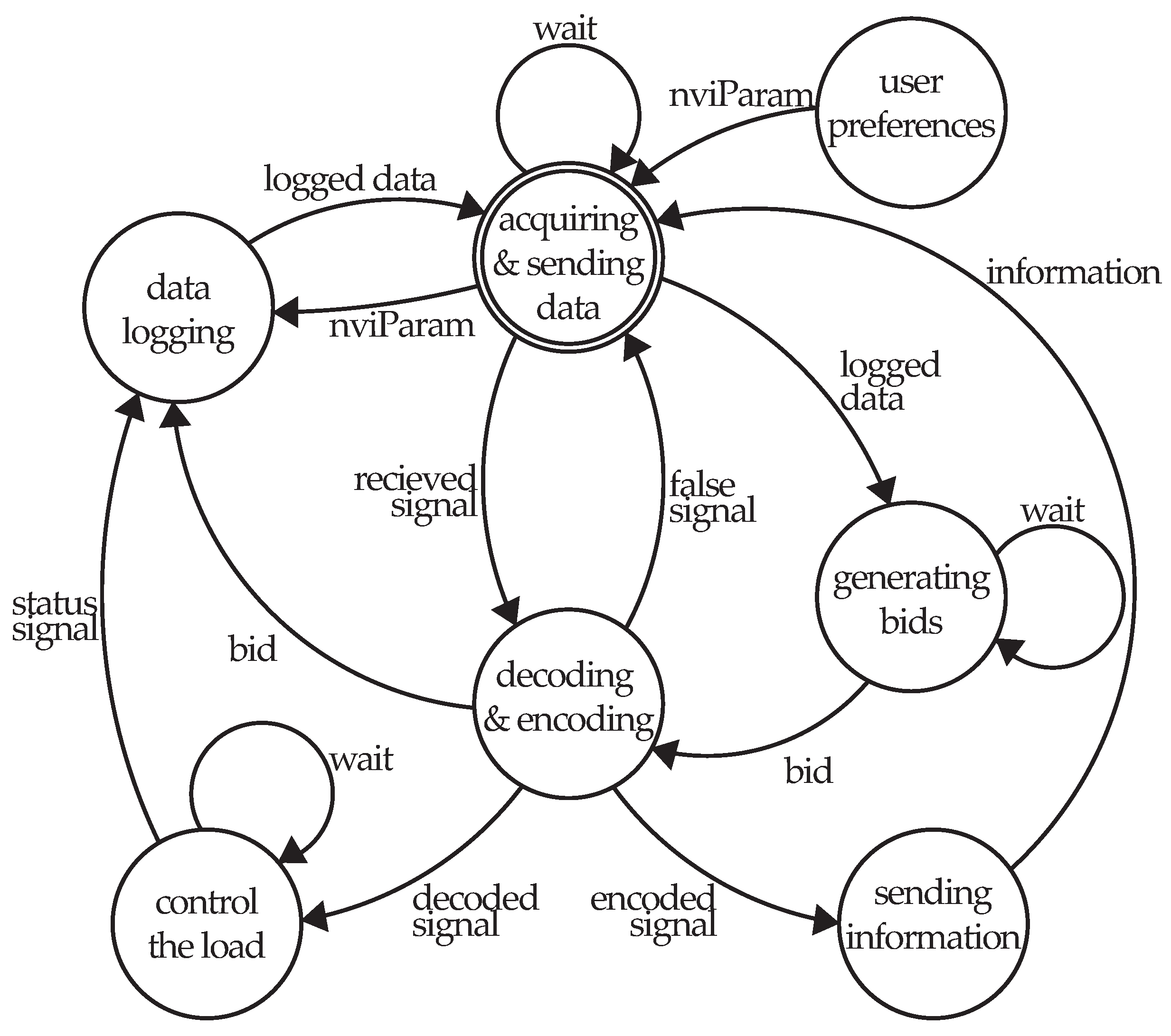
4.2. Finite State Machine
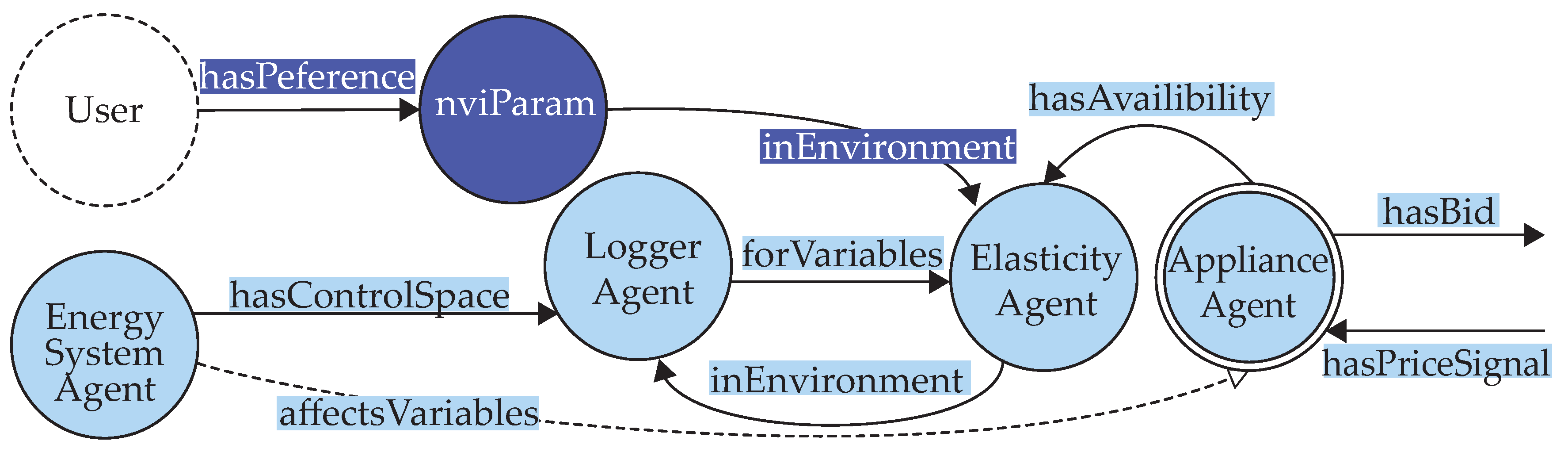
4.3. Knowledge Base
5. Evaluation
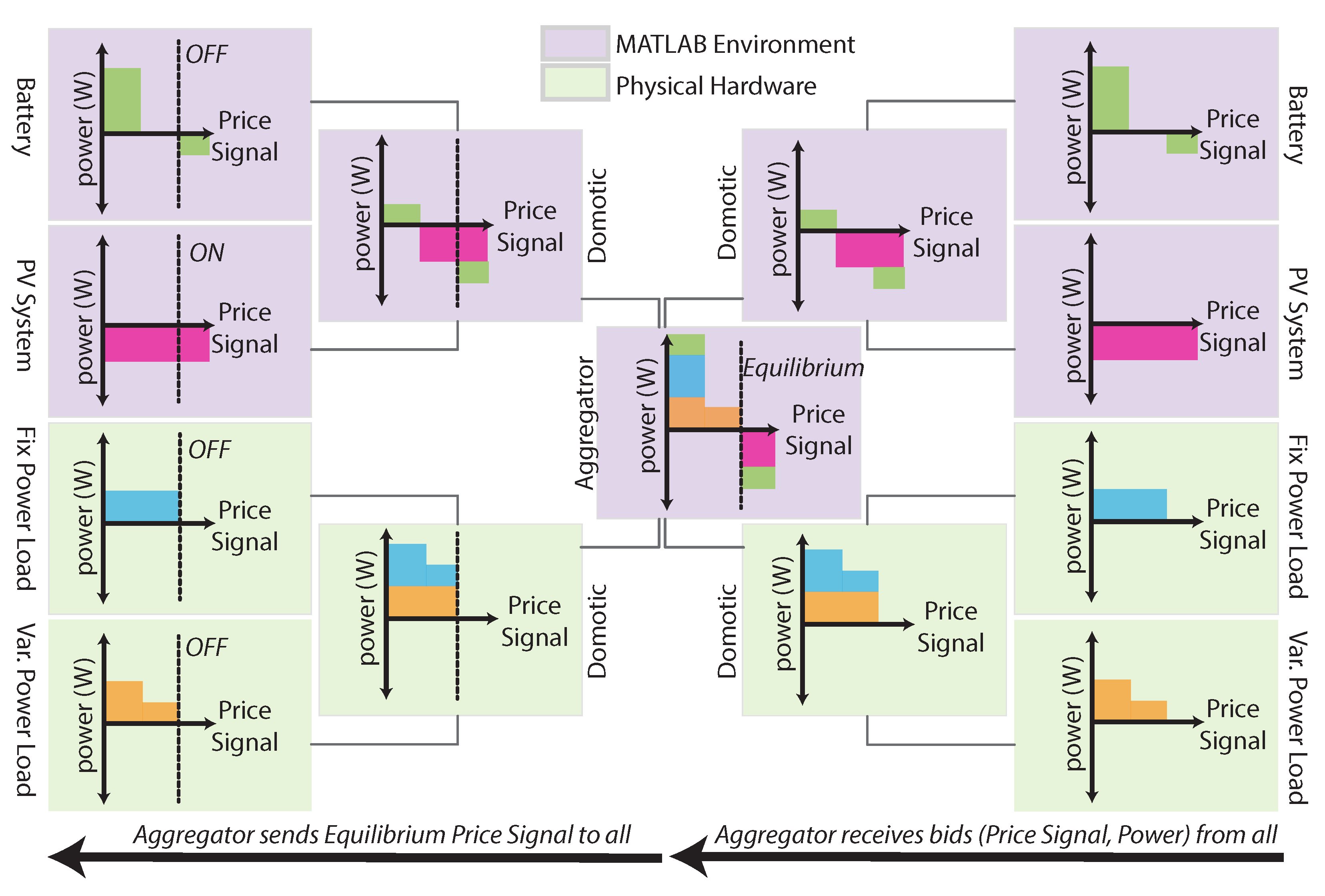
5.1. Experiment Design
5.2. Performance Metrics
5.3. Results
6. Conclusions
Acknowledgments
Author Contributions
Conflicts of Interest
References
- EIA. International Energy Outlook 2017 Overview. In IEO2017; EIA: Washington, DC, USA, 2017; Volume 143. [Google Scholar]
- Papaefthymiou, G.; Dragoon, K. Towards 100% renewable energy systems: Uncapping power system flexibility. Energy Policy 2016, 92, 69–82. [Google Scholar] [CrossRef]
- Parvathy, S.; Patne, N.R.; Jadhav, A.M. A smart demand side management mechanism for domestic energy consumers with major HVAC load. In Proceedings of the IEEE International Conference on Electrical Power and Energy Systems (ICEPES), Bhopal, India, 14–16 December 2016; pp. 504–511. [Google Scholar]
- Ożadowicz, A. A New Concept of Active Demand Side Management for Energy Efficient Prosumer Microgrids with Smart Building Technologies. Energies 2017, 10, 1771. [Google Scholar] [CrossRef]
- Bahrami, S.; Sheikhi, A. From demand response in smart grid toward integrated demand response in smart energy hub. IEEE Trans. Smart Grid 2016, 7, 650–658. [Google Scholar] [CrossRef]
- Fan, W.; Liu, N.; Zhang, J. An event-triggered online energy management algorithm of smart home: Lyapunov optimization approach. Energies 2016, 9, 381. [Google Scholar] [CrossRef]
- Melton, R.B. Gridwise Transactive Energy Framework (Draft Version); Technical Report; Pacific Northwest National Laboratory (PNNL): Richland, WA, USA, 2013. [Google Scholar]
- Liu, Z.; Wu, Q.; Huang, S.; Zhao, H. Transactive energy: A review of state of the art and implementation. In Proceedings of the 2017 IEEE Manchester PowerTech, Manchester, UK, 18–22 June 2017; pp. 1–6. [Google Scholar]
- Hu, J.; Yang, G.; Xue, Y. Economic Assessment of network-constrained transactive energy for managing flexible demand in distribution systems. Energies 2017, 10, 711. [Google Scholar] [CrossRef]
- Akter, M.N.; Mahmud, M.A.; Oo, A.M.T. A Hierarchical Transactive Energy Management System for Energy Sharing in Residential Microgrids. Energies 2017, 10, 2098. [Google Scholar] [CrossRef]
- Nunna, H.K.; Srinivasan, D. Multiagent-Based Transactive Energy Framework for Distribution Systems With Smart Microgrids. IEEE Trans. Ind. Inform. 2017, 13, 2241–2250. [Google Scholar] [CrossRef]
- Sijie, C.; Chen-Ching, L. From demand response to transactive energy: State of the art. J. Mod. Power Syst. Clean Energy 2017, 5, 10–19. [Google Scholar]
- Babar, M.; Nguyen, P.; Cuk, V.; Kamphuis, I. The development of demand elasticity model for demand response in the retail market environment. In Proceedings of the 2015 IEEE Eindhoven PowerTech, Eindhoven, The Netherlands, 29 June–2 July 2015; pp. 1–6. [Google Scholar]
- Ożadowicz, A.; Grela, J. An event-driven building energy management system enabling active demand side management. In Proceedings of the IEEE 2016 Second International Conference on Event-Based Control, Communication, and Signal Processing (EBCCSP), Krakow, Poland, 13–15 June 2016; pp. 1–8. [Google Scholar]
- Ożadowicz, A.; Grela, J.; Babar, M. Implementation of a demand elasticity model in the building energy management system. In Proceedings of the IEEE 2016 Second International Conference on Event-Based Control, Communication, and Signal Processing (EBCCSP), Krakow, Poland, 13–15 June 2016; pp. 1–4. [Google Scholar]
- Jachimski, M.; Mikoś, Z.; Wróbel, G.; Hayduk, G.; Kwasnowski, P. Event-based and time-triggered energy consumption data acquisition in building automation. In Proceedings of the IEEE 2015 International Conference on Event-Based Control, Communication, and Signal Processing (EBCCSP), Krakow, Poland, 17–19 June 2015; pp. 1–6. [Google Scholar]
- Simonov, M.; Chicco, G.; Zanetto, G. Event-driven energy metering: Principles and applications. IEEE Trans. Ind. Appl. 2017, 53, 3217–3227. [Google Scholar] [CrossRef]
- Lobaccaro, G.; Carlucci, S.; Löfström, E. A review of systems and technologies for smart homes and smart grids. Energies 2016, 9, 348. [Google Scholar] [CrossRef]
- Wang, Y.; Pordanjani, I.R.; Xu, W. An event-driven demand response scheme for power system security enhancement. IEEE Trans. Smart Grid 2011, 2, 23–29. [Google Scholar] [CrossRef]
- Collier, S.E. The emerging Enernet: Convergence of the smart grid with the internet of things. IEEE Ind. Appl. Mag. 2017, 23, 12–16. [Google Scholar] [CrossRef]
- Shaikh, P.H.; Nor, N.B.M.; Nallagownden, P.; Elamvazuthi, I.; Ibrahim, T. A review on optimized control systems for building energy and comfort management of smart sustainable buildings. Renew. Sustain. Energy Rev. 2014, 34, 409–429. [Google Scholar] [CrossRef]
- Kok, K. The Powermatcher: Smart Coordination for the Smart Electricity Grid. Ph.D. Thesis, Vrije Universiteit, Amsterdam, The Netherlands, 2013. [Google Scholar]
- Fernandes, F.; Morais, H.; Vale, Z.; Ramos, C. Dynamic load management in a smart home to participate in demand response events. Energy Build. 2014, 82, 592–606. [Google Scholar] [CrossRef]
- Lilis, G.; Van Cutsem, O.; Kayal, M. Building virtualization engine: A novel approach based on discrete event simulation. In Proceedings of the IEEE 2016 Second International Conference on Event-based Control, Communication, and Signal Processing (EBCCSP), Krakow, Poland, 13–15 June 2016; pp. 1–5. [Google Scholar]
- Sučić, B.; Anđelković, A.S.; Tomšić, Ž. The concept of an integrated performance monitoring system for promotion of energy awareness in buildings. Energy Build. 2015, 98, 82–91. [Google Scholar] [CrossRef]
- Klaassen, E.; Kobus, C.; Frunt, J.; Slootweg, J. Responsiveness of residential electricity demand to dynamic tariffs: Experiences from a large field test in the netherlands. Appl. Energy 2016, 183, 1065–1074. [Google Scholar] [CrossRef]
- Mahieu, J. Active Demand Side Management. Master’s Thesis, Hogeschool West-Vlaanderen, Ostend, Belgium, 2012. [Google Scholar]
- Nguyen, P.H.; Kling, W.L.; Ribeiro, P.F. Smart power router: A flexible agent-based converter interface in active distribution networks. IEEE Trans. Smart Grid 2011, 2, 487–495. [Google Scholar] [CrossRef]
- Islam, S.; Woyte, A.; Belmans, R.; Heskes, P.; Rooij, P. Investigating performance, reliability and safety parameters of photovoltaic module inverter: Test results and compliances with the standards. Renew. Energy 2006, 31, 1157–1181. [Google Scholar] [CrossRef]
- Biegel, B.; Andersen, P.; Stoustrup, J.; Madsen, M.B.; Hansen, L.H.; Rasmussen, L.H. Aggregation and control of flexible consumers—A real life demonstration. IFAC Proc. Vol. 2014, 47, 9950–9955. [Google Scholar] [CrossRef]
- Abrishambaf, O.; Faria, P.; Gomes, L.; Spínola, J.; Vale, Z.; Corchado, J.M. Implementation of a real-time microgrid simulation platform based on centralized and distributed management. Energies 2017, 10, 806. [Google Scholar] [CrossRef]
- Camarinha-Matos, L.M. Collaborative smart grids—A survey on trends. Renew. Sustain. Energy Rev. 2016, 65, 283–294. [Google Scholar] [CrossRef]
- Basu, K.; Hawarah, L.; Arghira, N.; Joumaa, H.; Ploix, S. A prediction system for home appliance usage. Energy Build. 2013, 67, 668–679. [Google Scholar] [CrossRef]
- Camacho, R.; Carreira, P.; Lynce, I.; Resendes, S. An ontology-based approach to conflict resolution in Home and Building Automation Systems. Expert Syst. Appl. 2014, 41, 6161–6173. [Google Scholar] [CrossRef]
- Ivan, G.; Genesi, C.; Espeche, J.M. Deliverable-2.2: MAS2TERING platform design document. MAS2TERING Multi-Agent Systems Holonic Platform Generic Components. Available online: http://www.mas2tering.eu/wp-content/uploads/2016/09/MAS2TERING_Deliverable_2.2_platform-design-document.pdf (accessed on 4 December 2017).
- Hassan, S.; Meritxell, V. Deliverable-3.1: Multi-agent systems holonic platform generic components. MAS2TERING Multi-Agent Systems Holonic Platform Generic Components. Available online: https://euagenda.eu/upload/publications/mas2tering-multi-agent-systems-holonic-platform-generic-components.pdf (accessed on 4 December 2017).
- Dibowski, H.; Ploennigs, J.; Kabitzsch, K. Automated design of building automation systems. IEEE Trans. Ind. Electron. 2010, 57, 3606–3613. [Google Scholar] [CrossRef]
- Lehmann, M.; Mai, T.L.; Wollschlaeger, B.; Kabitzsch, K. Design approach for component-based automation systems using exact cover. In Proceedings of the 2014 IEEE Emerging Technology and Factory Automation (ETFA), Barcelona, Spain, 16–19 September 2014; pp. 1–8. [Google Scholar]
- Jung, M.; Reinisch, C.; Kastner, W. Integrating building automation systems and ipv6 in the internet of things. In Proceedings of the IEEE 2012 Sixth International Conference on Innovative Mobile and Internet Services in Ubiquitous Computing (IMIS), Palermo, Italy, 4–6 July 2012; pp. 683–688. [Google Scholar]
- Lilis, G.; Conus, G.; Asadi, N.; Kayal, M. Towards the next generation of intelligent building: An assessment study of current automation and future IoT based systems with a proposal for transitional design. Sustain. Cities Soc. 2017, 28, 473–481. [Google Scholar] [CrossRef]
- Seldon, J.R. A note on the teaching of arc elasticity. J. Econ. Educ. 1986, 17, 120–124. [Google Scholar] [CrossRef]
- Babar, M.; Nguyen, P.; Cuk, V.; Kamphuis, I.; Bongaerts, M.; Hanzelka, Z. The evaluation of agile demand response: An applied methodology. IEEE Trans. Smart Grid 2017. [Google Scholar] [CrossRef]
- Watkins, C.J.; Dayan, P. Q-learning. Mach. Learn. 1992, 8, 279–292. [Google Scholar] [CrossRef]


| NV Name | Description |
|---|---|
| nviTimeSet | Synchronization and time settings for measurement purpose |
| nviEnergyClear | Reset or initialize the electricity consumption total |
| nviSwitch | Load control input—to provide external signals (e.g., an request for energy reduction sent by the provider to the customer in DR services) |
| Total active energy—meter value output | |
| nvoRegValueEnergy | Total active energy—this NV cannot be reset |
| nvoEnergyClearTime | Date and time of resetting nvoEnergy |
| nvoPower | Total active energy—meter value output |
| nvoVoltage | Phase voltage mean value |
| nvoCurrent | Phase current mean value |
| nvoFreq | Fundamental voltage frequency |
| nvoStatus | Device status report/info |
| nvoPowerUpHours | Operating hours since the last time operating at which the device was switched ON |
| nvoSwitch | Load control output—providing direct control of device or group of loads, taking into account demand analysis results, by changing the state of the relay actuator |
| cpParamSendDelta | Send on Delta send condition setting (Param can be energy, current, etc.) |
| cpParamMaxSendTime | Polling time send condition setting (Param can be energy, current, etc.) |
| cpLocation | Installation location and logger ID |
| NV Name | Description |
|---|---|
| nviTimeSet | Synchronization and time settings for logging purpose |
| nviResetEnergy | Reset or initialize the nvoEnergy |
| nviResetDemandPeak | Reset Demand Peak NVs |
| nviPeriodChoice | Historical period of when data are saved to the meter |
| nviTimeSelection | Historical time selection |
| nviEndPeriod | Measuring period ending input |
| nviRegisterState | Register state selection input |
| nviRegisterValue | Send value to the energy register object via the network |
| nvoEnergy | Total active energy—copy of the current meter value (for the last month). It could provide other historical data as well |
| nvoRegValueEnergy | Current value of the energy register with a time stamp and status bits |
| nvoEnergyHistTime | Register historical time output |
| nvoDemand | Demand power (average power over demand period) |
| nvoDemandPeak | Peak demand power |
| nvoDemandPeakTime | Time and date of peak demand |
| nvoMeasurePeriod | The length of the measuring period |
| nvoStatus | Device status report/info |
| cpLogMinutes | Logging interval. Default: 15 min |
| cpDemandPerMinutes | Demand period: 5 min to 1440 min. Default: 15 min |
| cpDemandSubinterval | Rolling demand subinterval count: 1–8. Default: 1 |
| cpHighLimit | Definition of the highest normal value of the register |
| cpBaseValue | Definition of the base value of the register |
| cpEnergyMaxSendTime | Polling time send condition setting (Param can be energy, current, etc.) |
| cpEnergySendDelta | Send on Delta send condition setting (Param can be energy, current, etc.) |
| cpRegisterName | Definition of the register name |
| cpLocation | Installation location and logger ID |
| NV Name | Description |
|---|---|
| nviTimeSet | Synchronization and time settings for learning purpose |
| nviDemand | Demand value input from IoT Energy Logger |
| nviPrice | Customer preferences parameter which may affect demand—Price |
| nviOccupancy | Customer preferences parameter which may affect demand—Occupancy |
| nviParam (start time) | Agent start time |
| nviParam (stop time) | Agent stop time |
| nviParam (etc…) | customer preferences input parameter which may affect demand |
| nvoExpDemand | Expected demand value (calculated) |
| nvoAbsError | Absolute error value (of calculation) |
| nvoAbsAction | Action value (of calculation)—control action to an agent (e.g., turn on/off lamp) |
| nvoStatus | Device status report/info |
| cpValueFunction | Setting: learner value function |
| cpExpRewardInterval | Send condition: maximum reward |
| cpStateSpace | Setting: triggerings actions |
| cpActionSpaceInterval | Send condition: nvoExpDemand |
| cpLocation | Installation location and logger ID |
| Flexometer | Without | With |
|---|---|---|
| with variable loading | 13 s | 7.0 s |
| with fixed loading | 4.9 s | 1.7 s |
© 2018 by the authors. Licensee MDPI, Basel, Switzerland. This article is an open access article distributed under the terms and conditions of the Creative Commons Attribution (CC BY) license (http://creativecommons.org/licenses/by/4.0/).
Share and Cite
Babar, M.; Grela, J.; Ożadowicz, A.; Nguyen, P.H.; Hanzelka, Z.; Kamphuis, I.G. Energy Flexometer: Transactive Energy-Based Internet of Things Technology. Energies 2018, 11, 568. https://doi.org/10.3390/en11030568
Babar M, Grela J, Ożadowicz A, Nguyen PH, Hanzelka Z, Kamphuis IG. Energy Flexometer: Transactive Energy-Based Internet of Things Technology. Energies. 2018; 11(3):568. https://doi.org/10.3390/en11030568
Chicago/Turabian StyleBabar, Muhammad, Jakub Grela, Andrzej Ożadowicz, Phuong H. Nguyen, Zbigniew Hanzelka, and I. G. Kamphuis. 2018. "Energy Flexometer: Transactive Energy-Based Internet of Things Technology" Energies 11, no. 3: 568. https://doi.org/10.3390/en11030568
APA StyleBabar, M., Grela, J., Ożadowicz, A., Nguyen, P. H., Hanzelka, Z., & Kamphuis, I. G. (2018). Energy Flexometer: Transactive Energy-Based Internet of Things Technology. Energies, 11(3), 568. https://doi.org/10.3390/en11030568