Smart Global Maximum Power Point Tracking Controller of Photovoltaic Module Arrays


1
Department of Electrical Engineering, National Changhua University of Education, Changhua 50074, Taiwan
2
Department of Electrical Engineering, National Chin-Yi University of Technology, Taichung 41170, Taiwan
*
Author to whom correspondence should be addressed.
Energies 2018, 11(3), 567; https://doi.org/10.3390/en11030567
Submission received: 15 January 2018
/
Revised: 13 February 2018
/
Accepted: 19 February 2018
/
Published: 6 March 2018
(This article belongs to the Section I: Energy Fundamentals and Conversion)
Abstract
:This study first explored the effect of shading on the output characteristics of modules in a photovoltaic module array. Next, a modified particle swarm optimization (PSO) method was employed to track the maximum power point of the multiple-peak characteristic curve of the array. Through the optimization method, the weighting value and cognition learning factor decreased with an increasing number of iterations, whereas the social learning factor increased, thereby enhancing the tracking capability of a maximum power point tracker. In addition, the weighting value was slightly modified on the basis of the changes in the slope and power of the characteristic curve to increase the tracking speed and stability of the tracker. Finally, a PIC18F8720 microcontroller was coordinated with peripheral hardware circuits to realize the proposed PSO method, which was then adopted to track the maximum power point of the power–voltage (P–V) output characteristic curve of the photovoltaic module array under shading. Subsequently, tests were conducted to verify that the modified PSO method exhibited favorable tracking speed and accuracy.
1. Introduction
The output power of a photovoltaic module array is affected by daylight intensity and temperature and thus exhibits a nonlinear characteristic. Therefore, a maximum power point tracking (MPPT) controller can be used to maintain the output power of such an array at the highest level. Currently, common tracking methods include the voltage feedback, constant voltage, power feedback, perturb and observe (P&O), and incremental conductance (INC) methods [1,2,3,4,5]. In particular, the voltage feedback method [1,2] requires first measuring the voltage at the maximum power point of an array under a specific temperature. This method is advantageous for simple interpretation but, when the atmospheric conditions change substantially, it cannot track the updated maximum power point. On the basis of the characteristic that the maximum power point is associated with similar voltage under various irradiations, the constant voltage method [1] tracks the maximum power point and involves easy control and simple calculation. However, this method also cannot track the updated maximum power point after the atmospheric conditions change substantially. The power feedback method [3] adopts the variation rates of the output power and voltage (dP/dV) to determine the maximum power point. This method decreases energy consumption and exhibits high overall efficiency, but the accuracy of the sensory modules involved is undesirable. The P&O method [4] perturbs a photovoltaic system by increasing or decreasing the voltage during a fixed cycle. When the output power is increased with increasing voltage during a cycle, the subsequent cycle involves further increasing the voltage; otherwise, the voltage is reduced. This method is advantageous for a simple framework and few measurement parameters, but it cannot accurately track the maximum power point. In addition, the solution obtained using the P&O method can oscillate near the maximum point, thus increasing tracking losses. The INC method [5] compares the static conductance and dynamic conductance of a photovoltaic array to determine the tracking direction. This method enables accurate control and fast responses but involves high computation and expensive controllers. Hence, a simpler fast-converging technique [6] is proposed to improve the drawbacks of INC method. The aforementioned maximum power point tracking method is inadequate for examining a photovoltaic module array with shaded or malfunctioning modules because the power–voltage (P–V) curve of the array can exhibit multiple peaks [7]; hence, using the aforementioned convention tracking methods might mistakenly identify a regional maximum point as the global maximum point.
In recent years, various scholars have proposed smart maximum power tracking techniques for photovoltaic module arrays, including the fuzzy control (FC) [8,9], genetic algorithm (GA) [10], neural network (NN) [11], artificial neural network (ANN) [12,13], and ant colony algorithm (ACA) [14,15] methods. In particular, the FC, NN, and ANN methods involve complex control processes and computation; hence, they are difficult to execute. The GA and ACA methods [10,14,15] can only be used to examine photovoltaic module arrays with single-peak output characteristic curves or nonshaded modules. The work proposed in [16] suggests a simple relationship to predict the correct position of the global maximum power point. However, this method can only be used to examine PV module array with two-peak output characteristics. A maximum power point tracking scheme based on the ripple correlation control (RCC) algorithm was proposed in [17]. However, this method can only be applied for multilevel inverters. Compared with the conventional methods, these methods enable higher success rates of identifying the global maximum power point.
Because the aforementioned MPPT techniques can only be used to examine photovoltaic module arrays with single-peak or two-peak output characteristic curves, this study employed and modified a particle swarm optimization (PSO) method. Under dissimilar shading ratios, the modified PSO method enabled effective identification of the global maximum power point of a photovoltaic module array with double-peak, triple-peak, and quadruple-peak P–V curves.
2. Characteristics of Photovoltaic Module Array
In a photovoltaic power generation system, photovoltaic modules are connected in parallel and series into an array to increase the output power of the system. However, when the module array is shaded by external factors such as clouds, trees, buildings, or stains, the output power curve of the system exhibits nonlinear variations and multiple peaks.
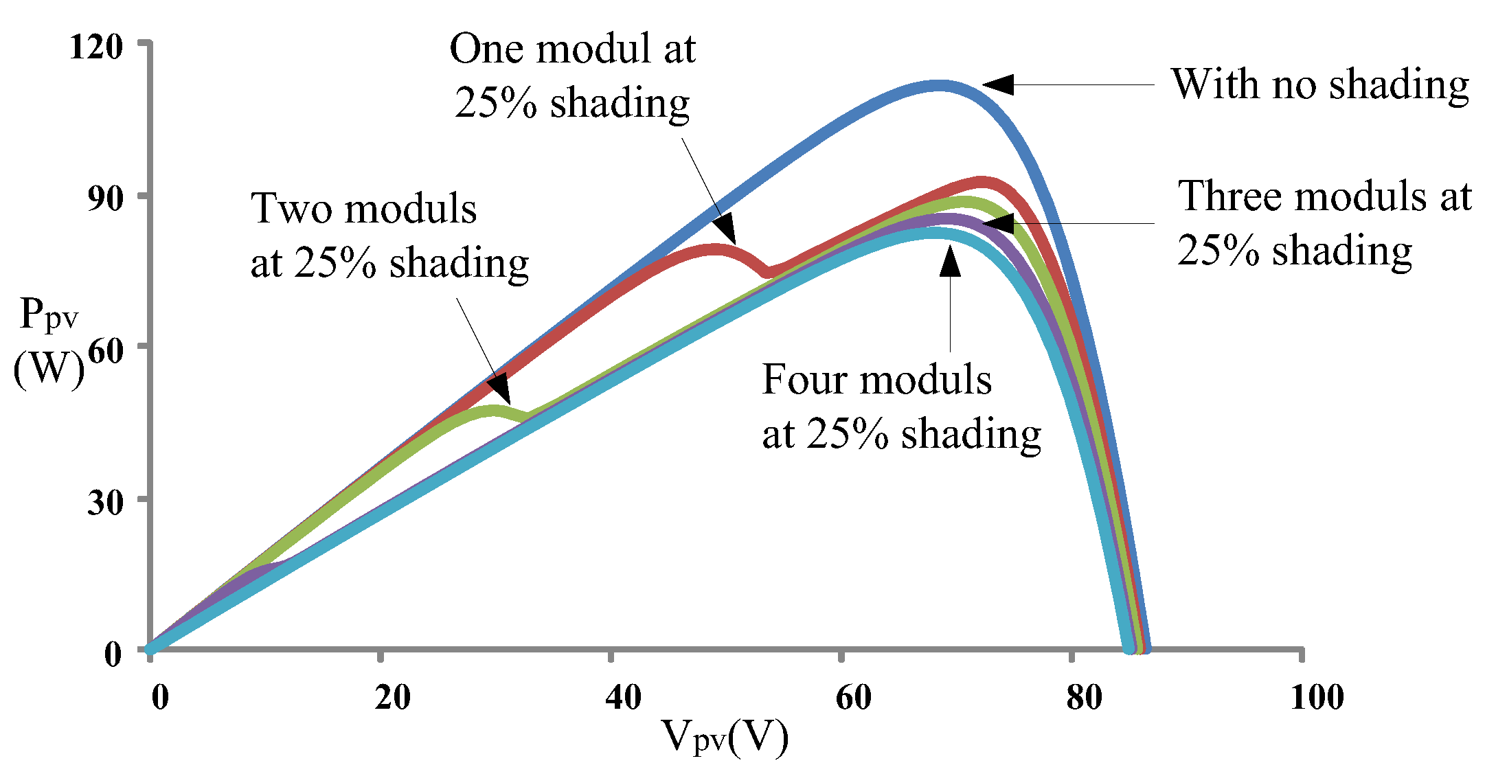
To investigate the output characteristic of a photovoltaic module array with several modules (connected in parallel or series) being shaded, this study connected Sanyo (Moriguchi, Osaka, Japan) HIP2727 modules to form a 4-series 1-parallel photovoltaic module array. Figure 1 and Figure 2 respectively illustrate the current–voltage (I–V) curve and power–voltage (P–V) curve simulated using Solar Pro software (R3.1, Laplace Systems, Kyoto, Japan) [18] when one, two, three, and four modules were at 25% shading. The results revealed that when several modules in the array were shaded, the output characteristic curve exhibited multiple peaks, and the maximum power point decreased with the increasing number of shaded modules.
3. Particle Swarm Optimization
PSO is a swarm intelligence optimization theory proposed by Eberhart and Kennedy [19] in 1995 and is categorized as a branch of evolutionary algorithms. The theory was inspired when the two scholars observed the foraging behavior of bird colonies; it is typically employed to solve related search and optimization problems [20,21]. In this theory, each flying bird in space is called a particle, and each moving particle is associated with an adequate value reflected through an objective function. In addition, the velocity of each particle determines its displacement and direction. When moving in space, the particles are affected by two types of memory value. Each particle searches and memorizes its individual current optimal location. The memory of each particle is accessible to other particles, enabling the particles to select the swarm optimal location from various individual optimal locations. Through this method, the particle swarm continuously modifies its velocity to quickly converge to the global optimal solution.
3.1. Conventional Particle Swarm Optimization
The process of the conventional PSO algorithm is described as follows:
- Step 1
- Configure the number of particles, maximum number of iterations, weighting value, and learning factors.
- Step 2
- Initialize the particle swarm and randomly configure the location and velocity of each particle.
- Step 3
- Substitute the initial location of each particle into an objective function to assess the fitness function value of each particle.
- Step 4
- Compare the fitness function value of each particle with its individual optimal memory location (Pbest,i) to select the more favorable value to update Pbest.
- Step 5
- Compare each Pbest value with the group optimal memory value (Gbest); if a Pbest value is more favorable than the Gbest value, the Gbest value is updated to the Pbest value.
- Step 6
- Use the kernel equations of PSO to update the particle velocity and location, as shown in Equations (1) and (2).
- Step 7
- Terminate the tracking process if the stop criterion is fulfilled. Otherwise, repeat Step 4 to 6 until fulfilling the stop criterion (identifying the global optimal solution) or researching the maximum iteration.
The parameters of the conventional PSO algorithm are elucidated as follows:
- Weighting value W: The W value of a particle is associated with its previous movement distance.
- Cognition learning factor (C1): The C1 value of a particle is related to itself.
- Social learning factor (C2): The C2 value of a particle is related to other particles.
- : the velocity of ith particle in jth iteration.
- : the location of ith particle in jth iteration.
- rand1(): the first random number generator, the value of which is between 0 and 1.
- rand2(): the second random number generator, the value of which is between 0 and 1.
- : the individual optimal solution of ith particle.
- : the group optimal solution.
The weighting value and learning factors of the PSO algorithm affects the success rate and tracking efficiency of the algorithm [22]. An excessively small weighting value yields an insufficient particle movement distance, and thus is unable to determine a global optimal solution from the regional optimal solutions of a multiple-peak curve. By contrast, an excessively large weighting value yields an extensive particle movement distance and thus fails to accurately identify the object function. Therefore, the weighting value is usually selected according to the object function. In addition, an excessively large learning factor requires additional iterations and thus decreases the overall tracking efficiency. Accordingly, the C1 and C2 values should not be overly large.
3.2. Modified Particle Swarm Optimization
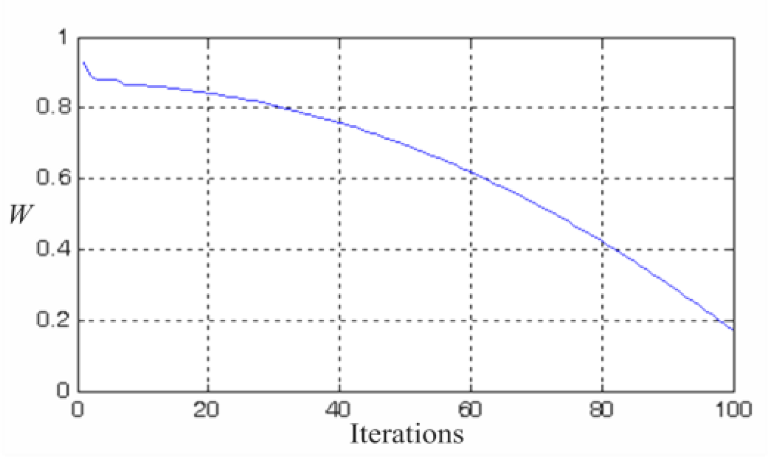
The PSO algorithm proposed in this study involves modifying the weighting of the conventional PSO. Specifically, Equation (3) is used to adjust the basic weighting and apply larger particle movements during the early iterations; this enables transcending of regional optimal solutions. However, as the number of iterations increases, the particles begin to closely approximate the global maximum power point; hence, the particle movement is reduced during this period to accurately track the global maximum power point.
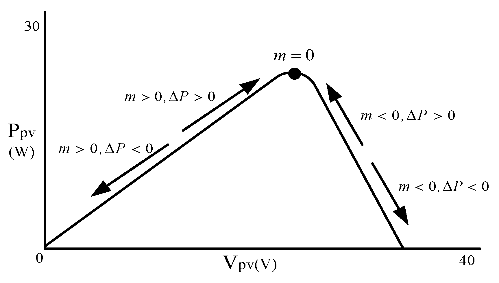
As shown in Figure 3, the power feedback method can be adopted to examine the slope (m) and changes in power () of the P–V characteristic curve of a photovoltaic module array. Figure 4 illustrates the trend of the weighting value according to m and , and Table 1 lists the criteria for adjusting the weighting value. Specifically, [(Wmax − Wmin)/2]/11 is used as the reference value for increasing or decreasing the weighting value, which is linearly adjusted according to the 11 ranges of the P–V curve slope. m and are defined using Equations (4) and (5):
- (1)
- m > 0 and a positive value indicate that the particles lie to the left of the maximum power point, with the tracking direction toward the maximum power point. A large m value implies that the particles are far away from the maximum power point; hence, the weighting value is increased to accelerate the tracking speed.
- (2)
- m < 0 and a positive value indicate that the particles lie to the right of the maximum power point, with the tracking direction toward the maximum power point. A small m value implies that the particles far away from the maximum power point; hence, the weighting value is increased to accelerate the tracking speed.
Parameters related to the weighting values are described as follows:
Upper limit of weighting (Wmax): the Wmax value of a particle is the maximum weighting value associated with its previous movement distance.
Lower limit of weighting (Wmin): the Wmin value of a particle is the minimum weighting value associated with its previous movement distance.
- : the current number of iterations.
- : the maximum number of iterations.
- P(j+1): the power yielded through j + 1 iterations.
- V(j+1): the voltage yielded through j + 1 iterations.
Regarding the learning factors, Equation (6) decreases the cognition learning factor C1 as the iteration number increases, indicating that reference to individual optimal locations is reduced with increasing iteration number. By contrast, Equation (7) increases the social learning factor C2 as the iteration number increases, indicating that reliance on the global optimal location is increased with increasing iteration number. Accordingly, the trends of the learning factors are displayed as in Figure 5 and Figure 6. Figure 7 illustrates the flowchart of the modified PSO algorithm. In this study, to ensure that the configured parameters of the modified PSO are not overly similar to those of the conventional PSO (Table 2) and thus affecting subsequent experimental interpretations, the upper limits of the weighting value, cognition learning factor, and social learning factor of the modified PSO were at least twice the values of the lower limits (Table 3).
Parameters related to the learning factors are defined as follows:
- C1,max: upper limit of cognition learning factor.
- C1,min: lower limit of cognition learning factor.
- C2,max: upper limit of social learning factor.
- C2,min: lower limit of social learning factor.
The weighting W was chosen to be 0.4 in the conventional PSO method for comparison with the modified PSO method using variable weighting. For the conventional PSO method, the weighting W is fixed at 0.4. However, the weighting is adjustable between Wmax (=0.9) and Wmin (=0.2) for the proposed modified PSO method according to the iteration times and the slope of P–V characteristic curve. And W = 0.4 is between the maximum value Wmax and the minimum value Wmin.
In this paper, the maximum power point tracking performance of the proposed modified PSO method and the conventional PSO method is compared. However, in the conventional PSO method, C1 and C2 are all selected as 2. Therefore, in the modified PSO method, the lower limit of C1 and C2 is also selected as 2, which is fair.
3.3. Framework of the Maximum Power Point Tracker of Modified Particle Swarm Optimization
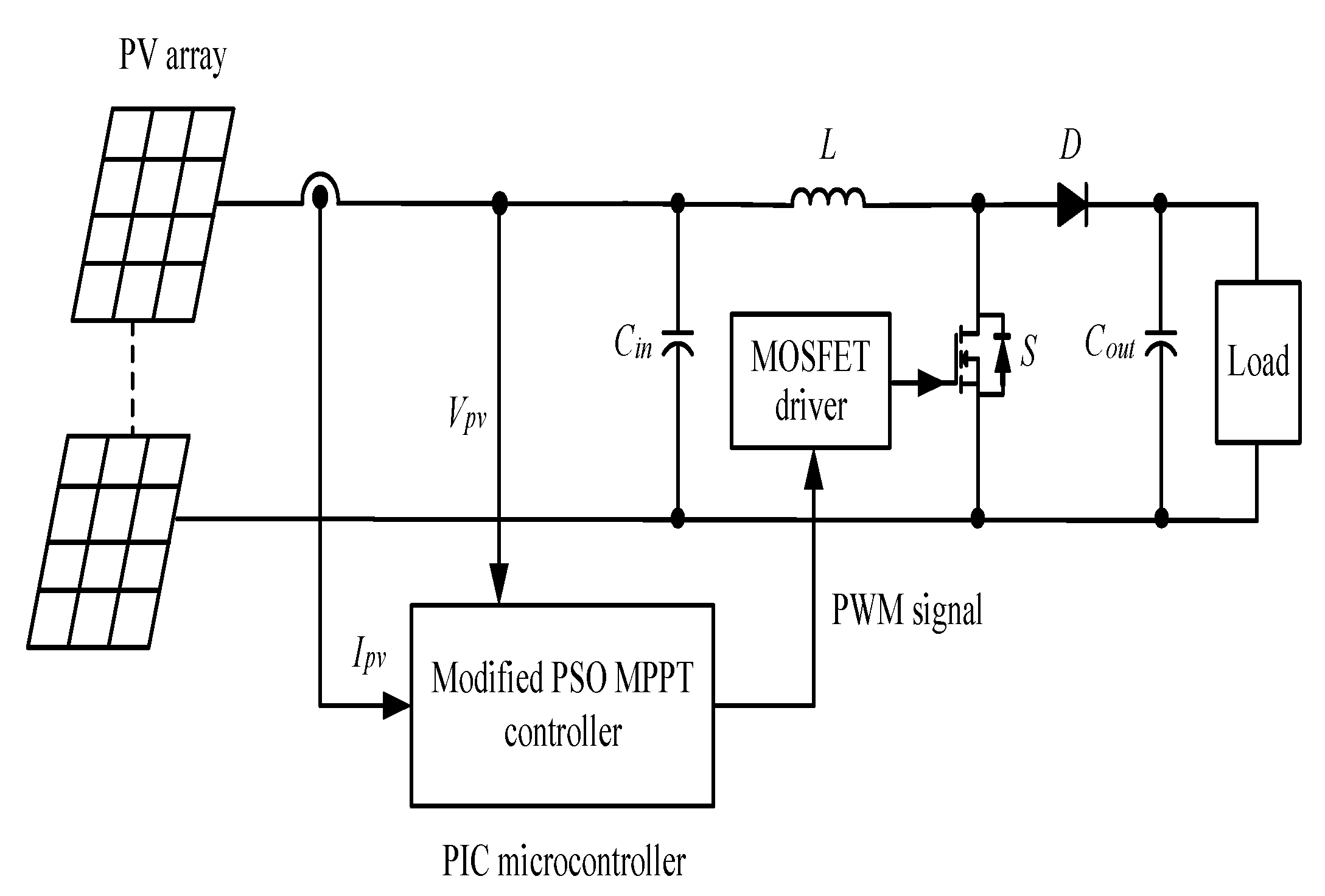
Figure 8 illustrates the framework of the maximum power point tracker of the modified PSO proposed in this study. The system includes a photovoltaic array arranged using Sanyo (Moriguchi, Osaka, Japan) HIP2717 modules [23], the PIC18F8720 microcontroller (R2004, Microchip Technology, Chandler, AZ, USA) [24], and a boost converter [25]. The modified PSO is used to control the duty cycle of the boost converter, thus identifying the global maximum power point of the module array. In particular, the tracking efficiency of this method is highlighted when the module array is shaded. Table 4 lists the parameter values of each component in the boost converter circuit. Table 5 lists the specifications of the HIP2717 module.
4. Testing Results of Conventional PSO and Modified PSO
In this study, the self-designed boost converter was integrated with the PIC microcontroller and coordinated with a HIP2717 simulator to examine the tracking capabilities of the conventional PSO and modified PSO trackers when they were applied to the photovoltaic module array under four cases of shading conditions, as listed in Table 6. Moreover, to accurately analyze the tracking capabilities of the two trackers under multiple peaks, the MP-170 measurement instrument was used [26]. Accordingly, the P–V characteristic curve of each case was plotted using the HIP2717 simulator.
(1) Case 1 (2-series 1-parallel: 0% shading + 40% shading)
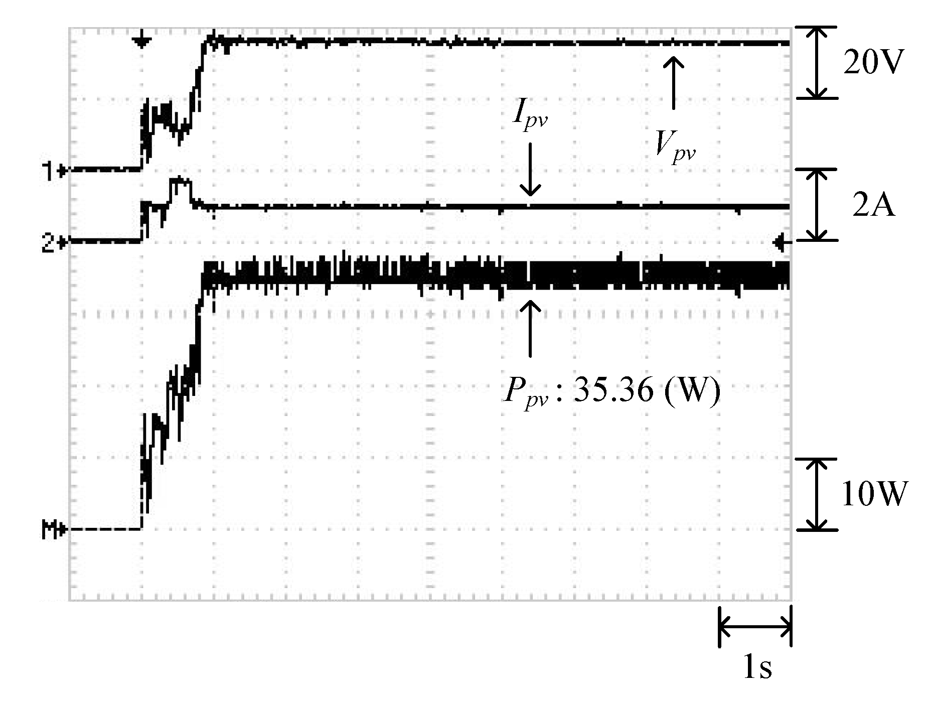
Figure 9 displays the P–V characteristic curve of Case 1 measured using MP-170. The curve exhibits two peaks, and the global maximum power point is located on the right peak (35.42 W). Figure 10 and Figure 11 illustrate the results obtained through the conventional and modified PSO algorithms, respectively. Comparing Figure 10 and Figure 11 revealed that the conventional PSO algorithm required more time to track the global maximum power point than the modified PSO algorithm.
(2) Case 2 (3-series 1-parallel: 0% shading + 30% shading + 70% shading)
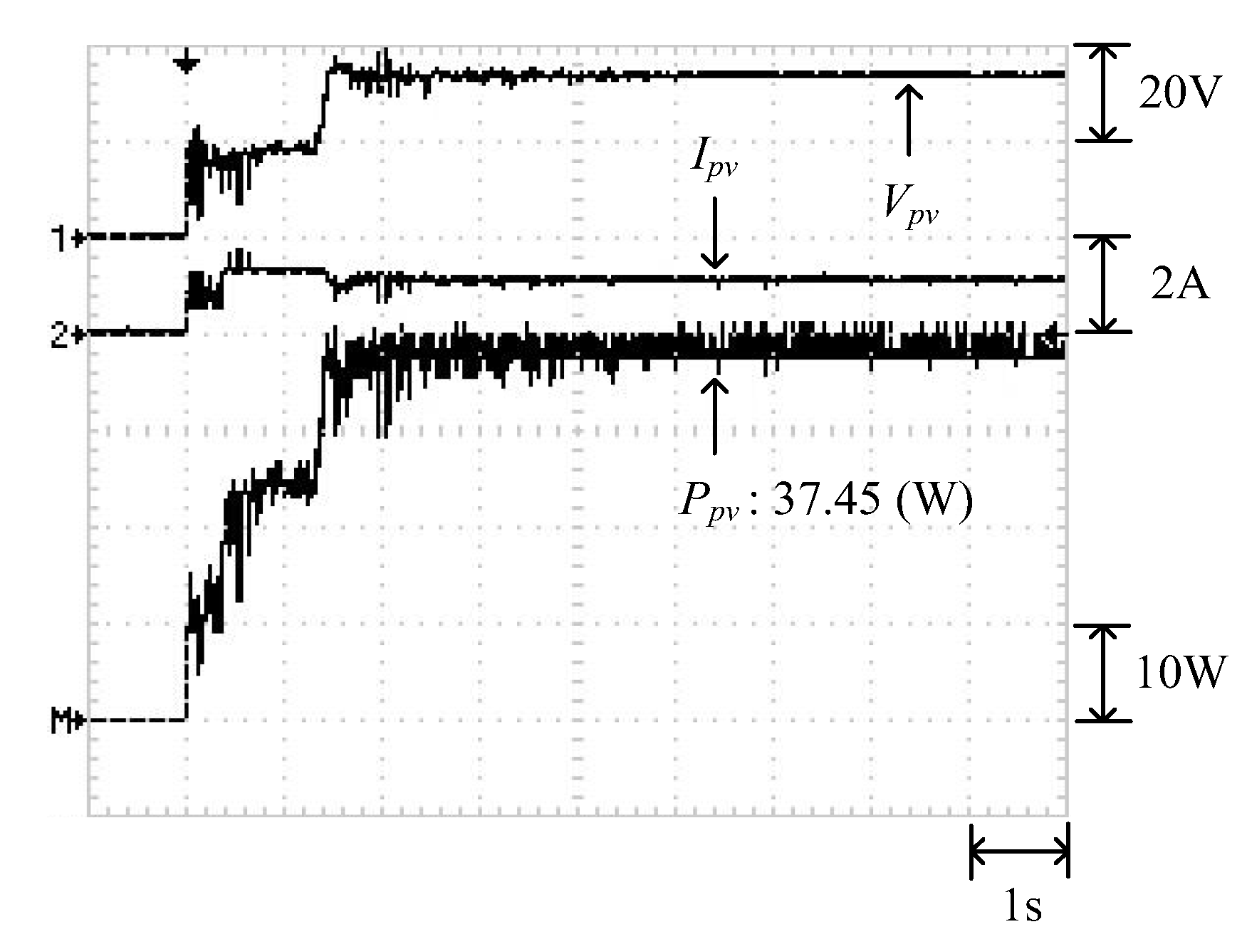
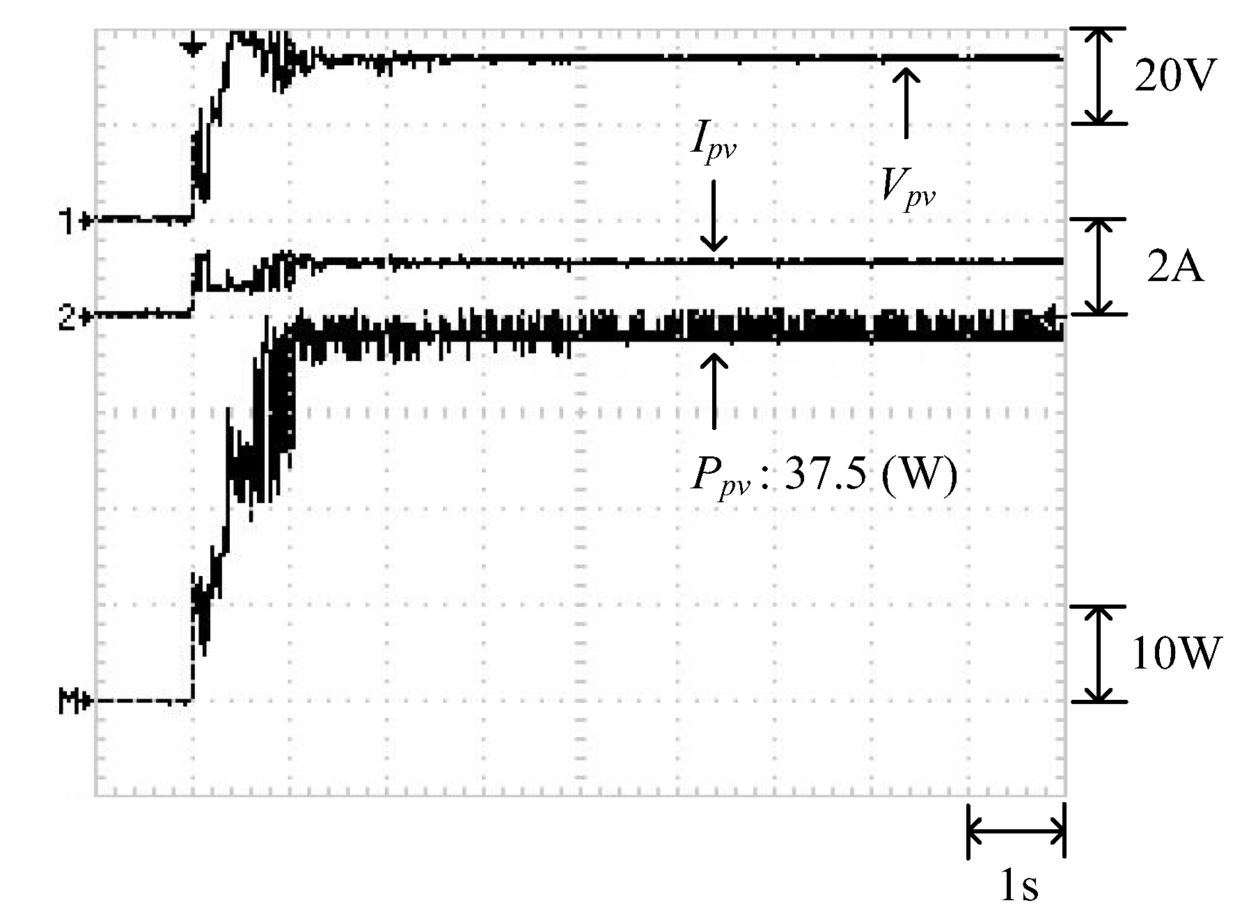
Figure 12 illustrates the P–V characteristic curve of Case 2. The curve demonstrates three peaks, with the global maximum power point located on the middle peak (37.52 W). Figure 13 and Figure 14 display the results obtained through the conventional and modified PSO algorithms, respectively. Observing these two figures showed that when the conventional PSO algorithm was used, additional time was required to transcend the regional solutions and track the global maximum power point (37.45 W). By contrast, the modified PSO algorithm required less time to transcend the regional solutions and accurately track the maximum power point (37.5 W).
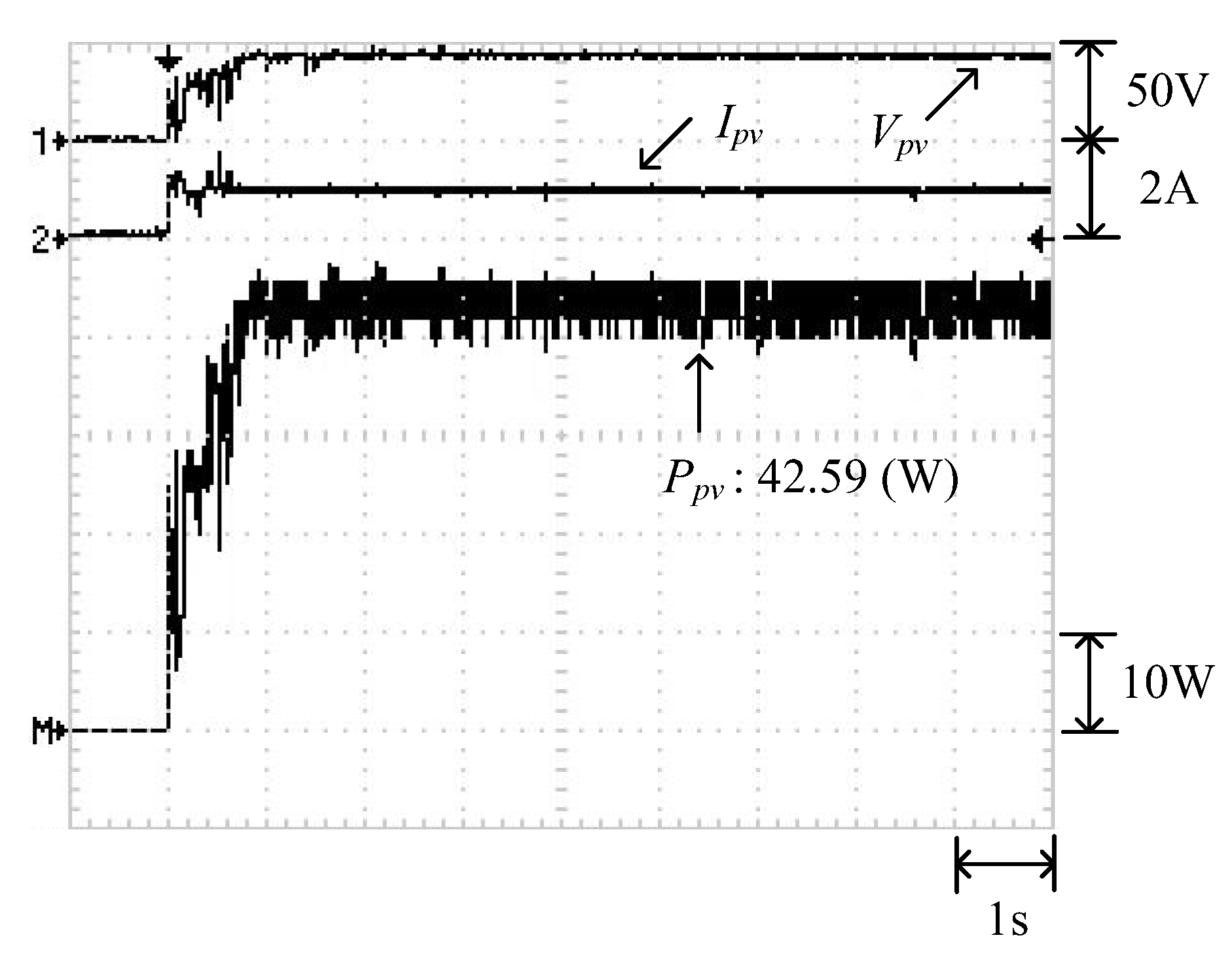
(3) Case 3 (4-series 1-parallel: 0% shading + 30% shading + 50% shading + 70% shading)
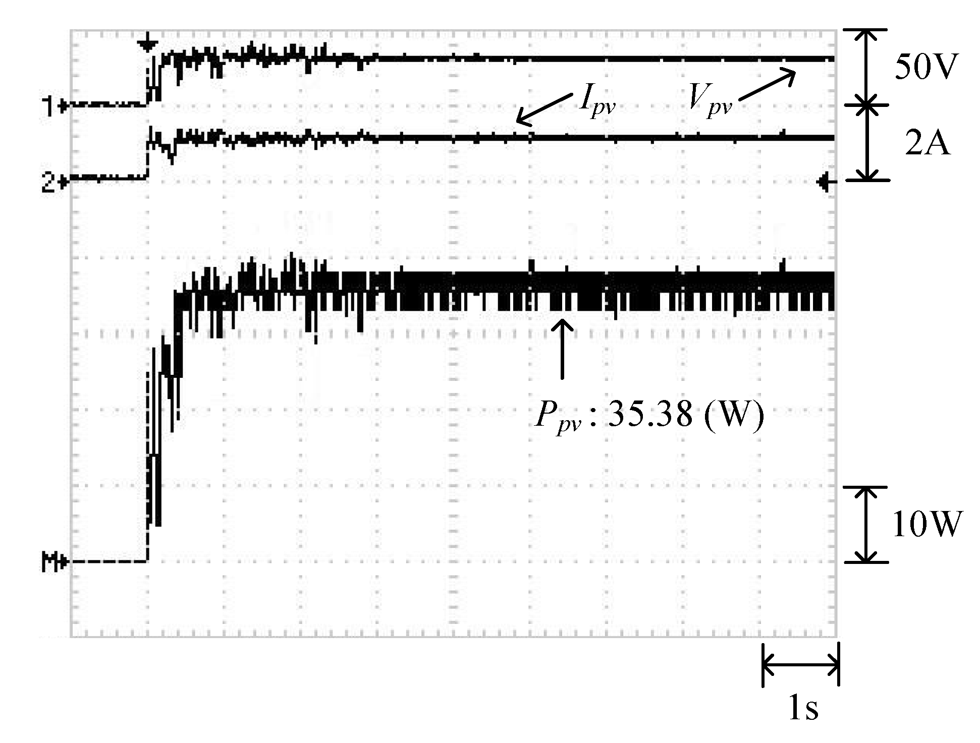
Figure 15 displays the P–V characteristic curve of Case 3. The curve exhibits four peaks, and the global maximum power point is located on the middle peak (42.9 W). Figure 16 and Figure 17 display the results obtained through the conventional and modified PSO algorithms, respectively. Comparing these two figures revealed that when the conventional PSO algorithm was used, the configured iteration number failed to transcend the local solutions, and the global maximum power point was inaccurately determined to be 35.38 W. By contrast, the modified PSO algorithm enabled quick transcending of regional solutions and tracking of the maximum power point (42.59 W), with favorable accuracy.
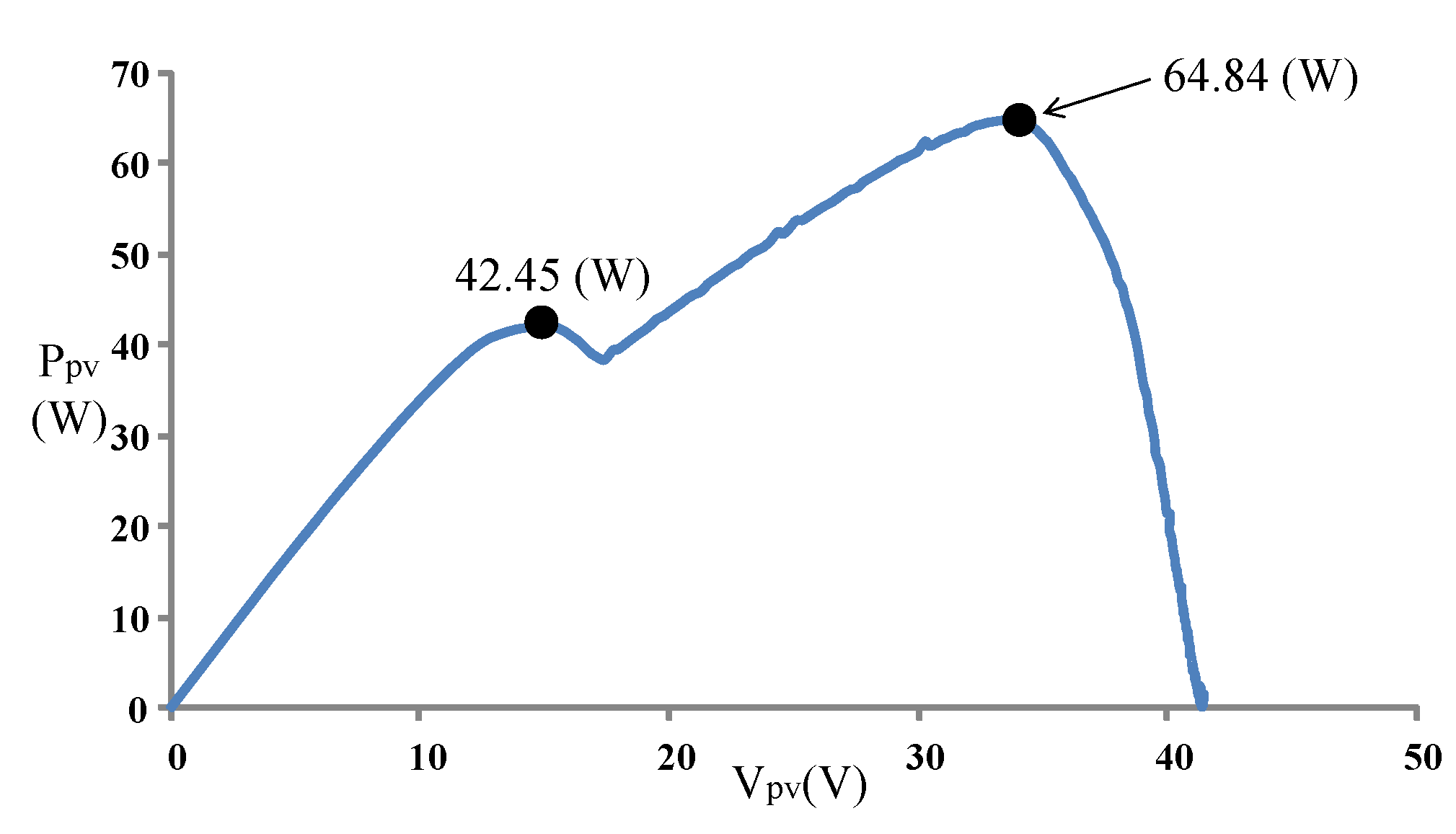
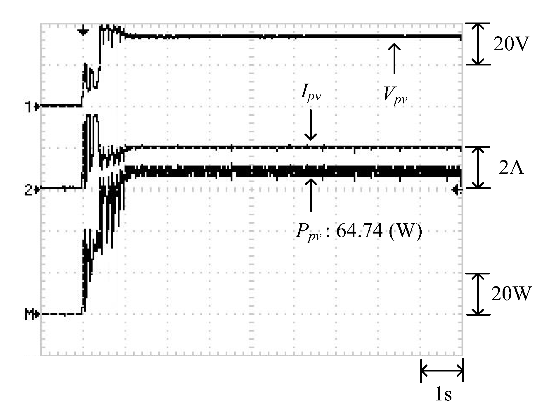
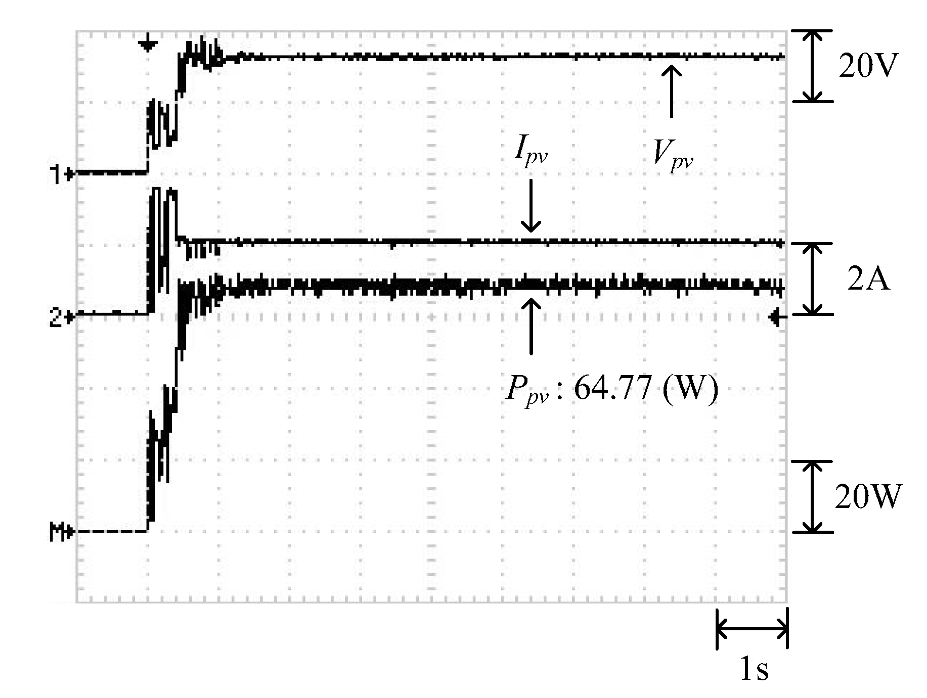
(4) Case 4 (2-series 2-parallel: (25% shading + 0% shading) // (55% shading + 0% shading))
Figure 18 illustrates the P–V characteristic curve of Case 4. The curve exhibits two peaks, and the global maximum power point is located on the right peak (64.84 W). Figure 19 and Figure 20 illustrate the results obtained through the conventional and modified PSO algorithms, respectively. Observing these two figures showed that the conventional PSO algorithm not only required additional time to transcend regional solutions but was also affected by the noise signals on the P–V curve. Therefore, the solution oscillated near 60 W before determining the global maximum power point. By contrast, the modified PSO algorithm enabled quick transcending of regional solutions, and the tracking and interpretation process was less affected by the noise signals.
(5) Comparison and analysis of each case
The four cases were each tested five times using the conventional PSO and modified PSO algorithms, and the tracking times and maximum power point values were averaged for each case, as shown in Table 7. The iterations of the two methods are all set as 100 times. They have been presented in Table 2 and Table 3, respectively. In this table, the average tracking time and average maximum power are derived through averaging tracking times and maximum power outputs of the five trials. The results showed that the average tracking time and maximum power of each case obtained through the modified PSO algorithm were more favorable than those attained through the conventional PSO algorithm.
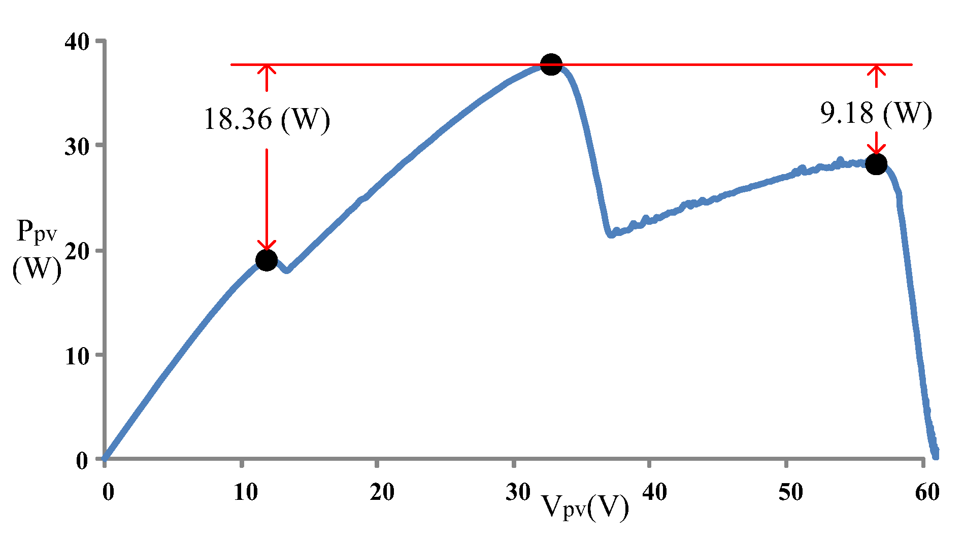
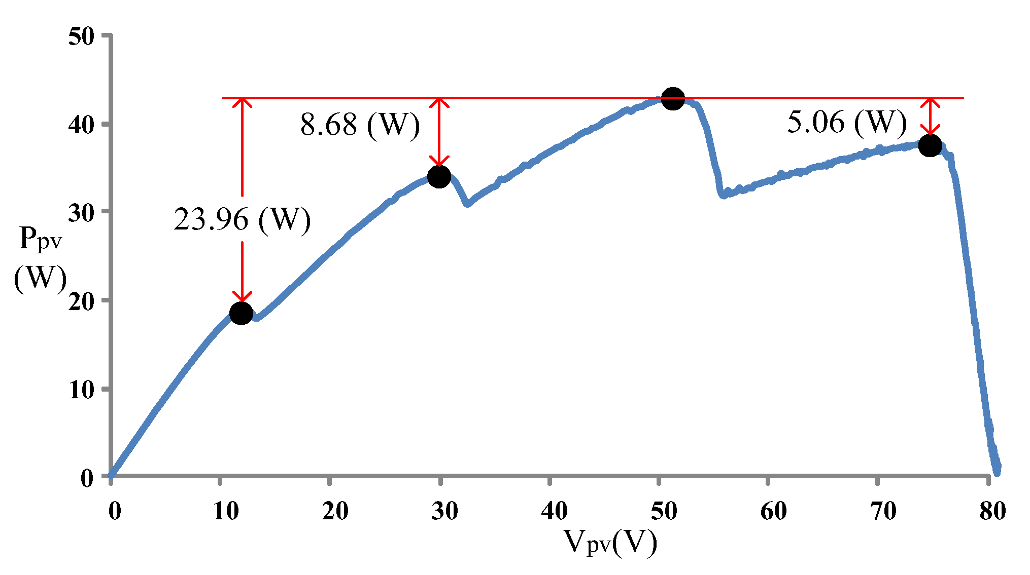
The test results verified that for each case, the modified PSO algorithm attained more favorable tracking speed and accuracy than did the convention PSO algorithm. Furthermore, using the conventional PSO algorithm failed to track the global maximum power point in Case 3. Therefore, the P–V characteristic curves of Case 2 and Case 3 were further analyzed (Figure 21 and Figure 22). The results showed that in Case 2, the global maximum power point differed from the left and right regional solutions by 18.36 W and 9.18 W, respectively. In Case 3, the global maximum power point differed from the three regional solutions by 23.96 W, 8.68 W, and 5.06 W (from the leftmost to rightmost peaks, respectively). Although both cases exhibited multiple-peak curves, two of the regional solutions in Case 3 closely approximated the global maximum power point. This facilitated incorrect identification of regional solutions as the global solution. Accordingly, the conventional PSO algorithm performed least desirably in Case 3.
5. Conclusions
In this study, the conventional PSO algorithm was adjusted to propose a modified PSO algorithm, which was then adopted to track the maximum power point of a photovoltaic module array. The weighting value, cognition learning factor, and social learning factor either increased or decreased with increasing iteration number. This facilitated decreasing the total number of iterations. In addition, the weighting value was slightly adjusted according to the slope and changes in power of the P–V characteristic curve, thus enhancing the success rate of tracking the global maximum power point. The test results verified that when the modules of the photovoltaic module arrays were partially shaded, the modified PSO algorithm more accurately and quickly tracked the global maximum power point than the conventional PSO algorithm.
Acknowledgments
The authors gratefully acknowledge the support of the Ministry of Science and Technology, Taiwan, under the Grant Number MOST 106-2221-E-167-013-MY2.
Author Contributions
The mode analysis on the maximum power point of the multiple-peak characteristic curve of the array was made by Long-Yi Chang. Jia-Jing Kao carried out the simulations and experiments of the proposed converter. Kuei-Hsiang Chao was responsible for writing the paper and serves as the corresponding author. Yi-Nung Chung implemented the boost converter and measured steady-state performance of the proposed converter.
Conflicts of Interest
The authors declare no conflict of interest.
References
- Tofoli, F.L.; Pereira, D.C.; Paula, W.J. Comparative Study of Maximum Power Point Tracking Techniques for Photovoltaic Systems. Int. J. Photoenergy 2015, 2015, 812582. [Google Scholar] [CrossRef]
- Masoum, M.A.S.; Dehbonei, H.; Fuchs, E.F. Theoretical and Experimental Analyses of Photovoltaic Systems with Voltage and Current-based Maximum Power Point Tracking. IEEE Trans. Energy Convers. 2002, 17, 514–522. [Google Scholar] [CrossRef]
- Subudhi, B.; Pradhan, R.A. Comparative Study on Maximum Power Point Tracking Techniques for Photovoltaic Power Systems. IEEE Trans. Sustain. Energy 2013, 4, 89–98. [Google Scholar] [CrossRef]
- Elgendy, M.A.; Zahawi, B.; Atkinson, D.J. Assessment of Perturb and Observe MPPT Algorithm Implementation Techniques for PV Pumping Applications. IEEE Trans. Sustain. Energy 2012, 3, 21–33. [Google Scholar] [CrossRef]
- Visweswara, K. An Investigation of Incremental Conductance Based Maximum Power Point Tracking for Photovoltaic System. Energy Procedia 2014, 54, 11–20. [Google Scholar] [CrossRef]
- Soon, T.K.; Mekhilef, S. A Fast-converging MPPT Technique for Photovoltaic System under Fast-varying Solar Irradiation and Load Resistance. IEEE Trans. Ind. Inf. 2016, 11, 176–186. [Google Scholar] [CrossRef]
- Moballegh, S.; Jiang, J. Modeling, Prediction, and Experimental Validations of Power Peaks of PV Arrays under Partial Shading Conditions. IEEE Trans. Sustain. Energy 2014, 5, 293–300. [Google Scholar] [CrossRef]
- Khateb, A.E.; Rahim, N.A.; Selvaraj, J.; Uddin, M.N. Fuzzy-logic-controller-based SEPIC Converter for Maximum Power Point Tracking. IEEE Trans. Ind. Appl. 2014, 50, 2349–2358. [Google Scholar] [CrossRef]
- Algarín, C.R.; Giraldo, J.T.; Álvarez, O.R. Fuzzy Logic Based MPPT Controller for a PV System. Energies 2017, 10, 2036. [Google Scholar] [CrossRef]
- Kumar, P.; Jain, G.; Palwalia, D.K. Genetic Algorithm Based Maximum Power Tracking in Solar Power Generation. In Proceedings of the International Conference on Power and Advanced Control Engineering (ICPACE), Bangalore, India, 12–14 August 2015; pp. 1–6. [Google Scholar]
- Veerachary, M.; Senjyu, T.; Uezato, K. Neural Network Based Maximum Power Point Tracking of Coupled Inductor Interleaved Boost Converter Supplied PV System Using Fuzzy Controller. IEEE Trans. Ind. Electron. 2003, 50, 749–758. [Google Scholar] [CrossRef]
- Khanaki, R.; Radzi, M.A.M.; Marhaban, M.H. Artificial Neural Network Based Maximum Power Point Tracking Controller for Photovoltaic Standalone System. Int. J. Green Energy 2016, 13, 283–291. [Google Scholar] [CrossRef]
- Ma, S.L.; Chen, M.X.; Wu, J.W.; Huo, W.L.; Huang, L. Augmented Nonlinear Controller for Maximum Power-Point Tracking with Artificial Neural Network in Grid-Connected Photovoltaic Systems. Energies 2016, 9, 1005. [Google Scholar] [CrossRef]
- Besheer, A.H. Ant Colony System Based PI Maximum Power Point Tracking for Standalone Photovoltaic System. In Proceedings of the IEEE International Conference on Industrial Technology, Athens, Greece, 19–21 March 2012; pp. 693–698. [Google Scholar]
- Nivetha, V.; Gowri, G.V. Maximum Power Point Tracking of Photovoltaic System Using Ant Colony and Particle Swam Optimization Algorithms. In Proceedings of the 2nd International Conference on Electronics and Communication Systems (ICECS), Coimbatore, India, 26–27 February 2015; pp. 948–952. [Google Scholar]
- Ahmed, J.; Salam, Z. An Improved Method to Predict the Position of Maximum Power Point during Partial Shading for PV Arrays. IEEE Trans. Ind. Inf. 2015, 11, 1378–1387. [Google Scholar] [CrossRef]
- Hammami, M.; Grandi, G. A Single-Phase Multilevel PV Generation System with an Improved Ripple Correlation Control MPPT Algorithm. Energies 2017, 10, 2037. [Google Scholar] [CrossRef]
- Solar Pro Official Website. Available online: http://lapsys.co.jp/english (accessed on 10 May 2016).
- Kennedy, J.; Eberhart, R.C. Particle Swarm Optimization. In Proceedings of the IEEE International Conference on Neural Networks, Perth, Australia, 27 November–1 December 1995; pp. 1942–1948. [Google Scholar]
- Eberhart, R.C.; Kennedy, J. A New Optimizer Using Particle Swarm Theory. In Proceedings of the Sixth International Symposium on Micro Machine and Human Science, Nagoya, Japan, 4–6 October 1995; pp. 39–43. [Google Scholar]
- Chao, K.H.; Lin, Y.S.; Lai, U.D. Improved Particle Swarm Optimization for Maximum Power Point Tracking in Photovoltaic Module Arrays. Appl. Energy 2015, 158, 609–618. [Google Scholar] [CrossRef]
- Han, W.H. Comparison Study of Several Kinds of Inertia Weights for PSO. In Proceedings of the IEEE International Conference on Informatics and Computing, Shanghai, China, 10–12 December 2010; pp. 280–284. [Google Scholar]
- SANYO HIP 2017 Datasheet. Available online: http://iris.nyit.edu/~mbertome/solardecathlon/SDClerical/SD_DESIGN+DEVELOPMENT/091804_Sanyo190HITBrochure.pdf (accessed on 15 January 2016).
- PIC18Fxx20 Datasheet. Available online: http://pdf.datasheetcatalog.com/datasheet/microchip/39609b.pdf (accessed on 15 July 2014).
- Hart, D.W. Introduction to Power Electronics; Prentice Hall: New York, NY, USA, 2003. [Google Scholar]
- MP-170 Brochure. Available online: http://www.environmental-expert.com/products/model-mp-170-iv-checker-80092 (accessed on 15 July 2014).
Figure 1.
Current–voltage (I–V) curves of the 4-series 1-parallel array when different numbers of modules were at 25% shading.
Figure 1.
Current–voltage (I–V) curves of the 4-series 1-parallel array when different numbers of modules were at 25% shading.
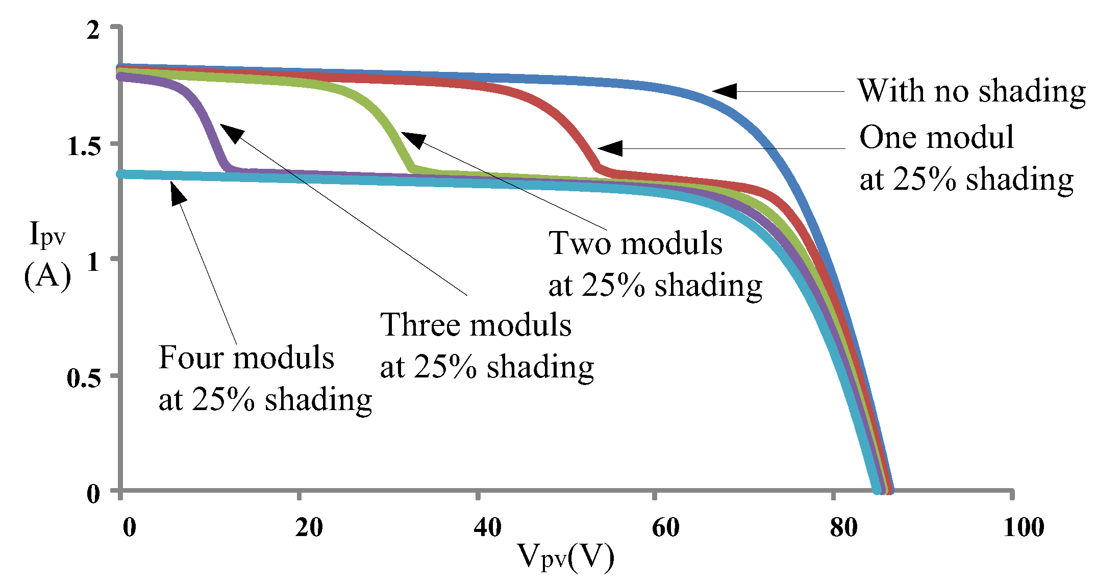
Figure 2.
Power–voltage (P–V) curves of the 4-series 1-parallel array when different numbers of modules were at 25% shading.
Figure 2.
Power–voltage (P–V) curves of the 4-series 1-parallel array when different numbers of modules were at 25% shading.

Figure 3.
Slope (m) and changes in power () of the P–V characteristic curve determined through the power feedback method.
Figure 3.
Slope (m) and changes in power () of the P–V characteristic curve determined through the power feedback method.

Figure 4.
Trends of the weighting value (W) of the modified particle swarm optimization (PSO).

Figure 5.
Trend of the cognition learning factor (C1) of the modified PSO.
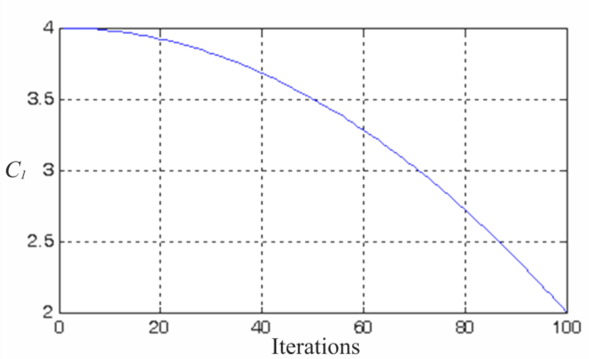
Figure 6.
Trend of the social learning factor (C2) of the modified PSO.
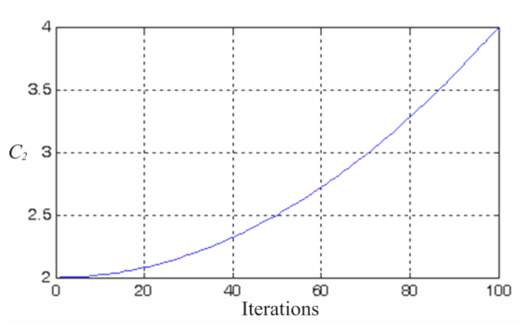
Figure 7.
Flowchart of the modified PSO algorithm.
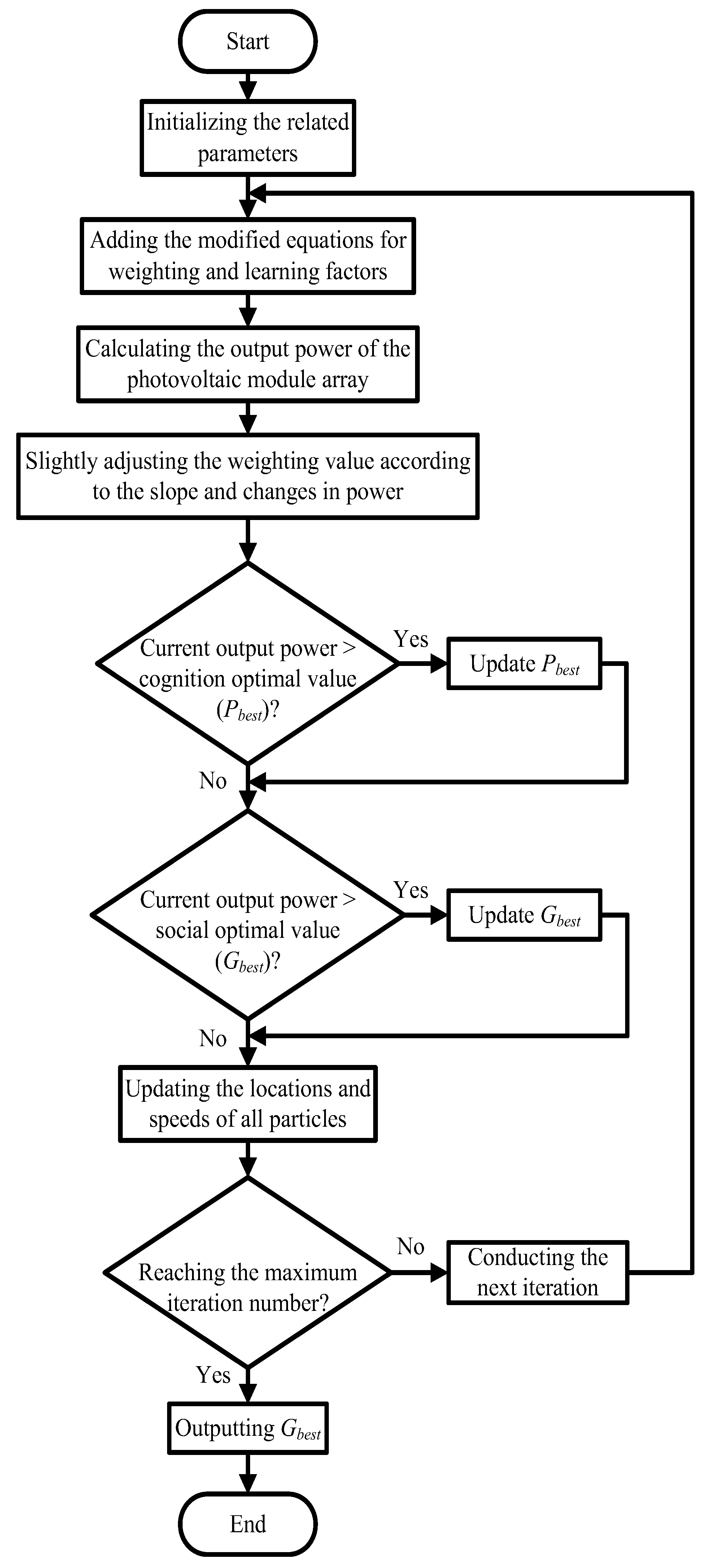
Figure 8.
Framework of the maximum power point tracker of the modified PSO.

Figure 9.
P–V characteristic curve of Case 1.
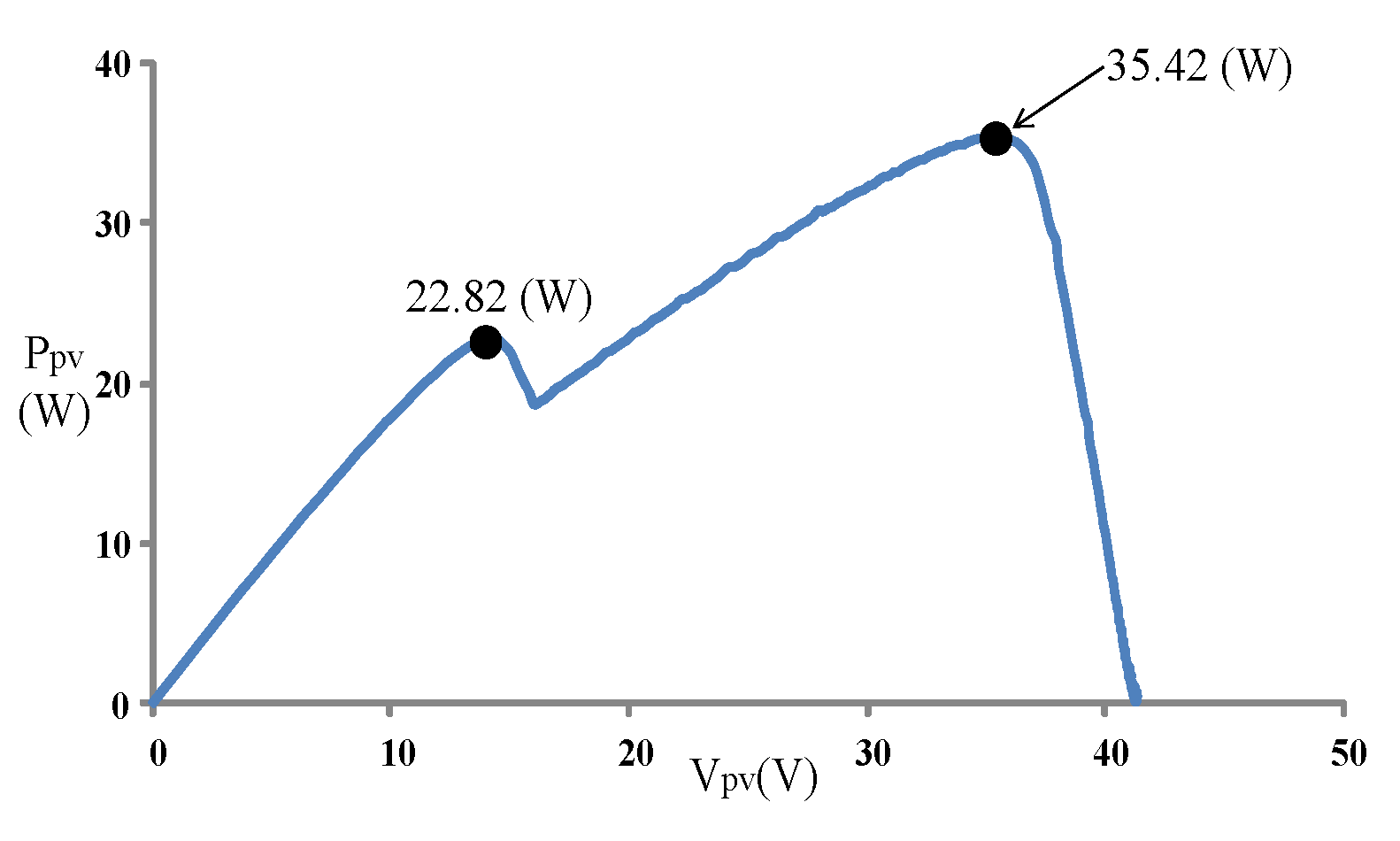
Figure 10.
Maximum power point of Case 1 determined through the conventional PSO algorithm.

Figure 11.
Maximum power point of Case 1 determined through the modified PSO algorithm.
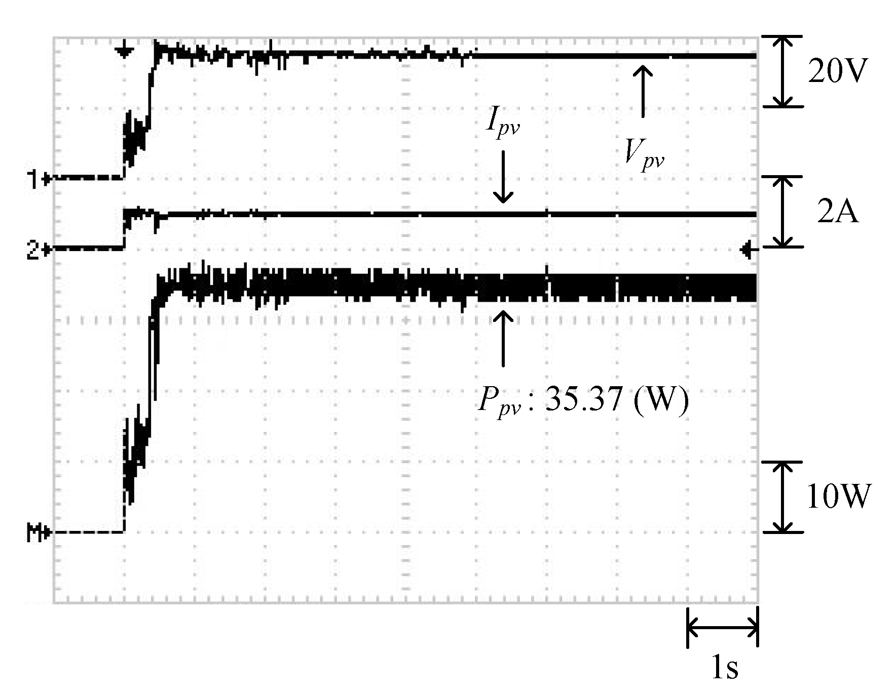
Figure 12.
P–V characteristic curve of Case 2.
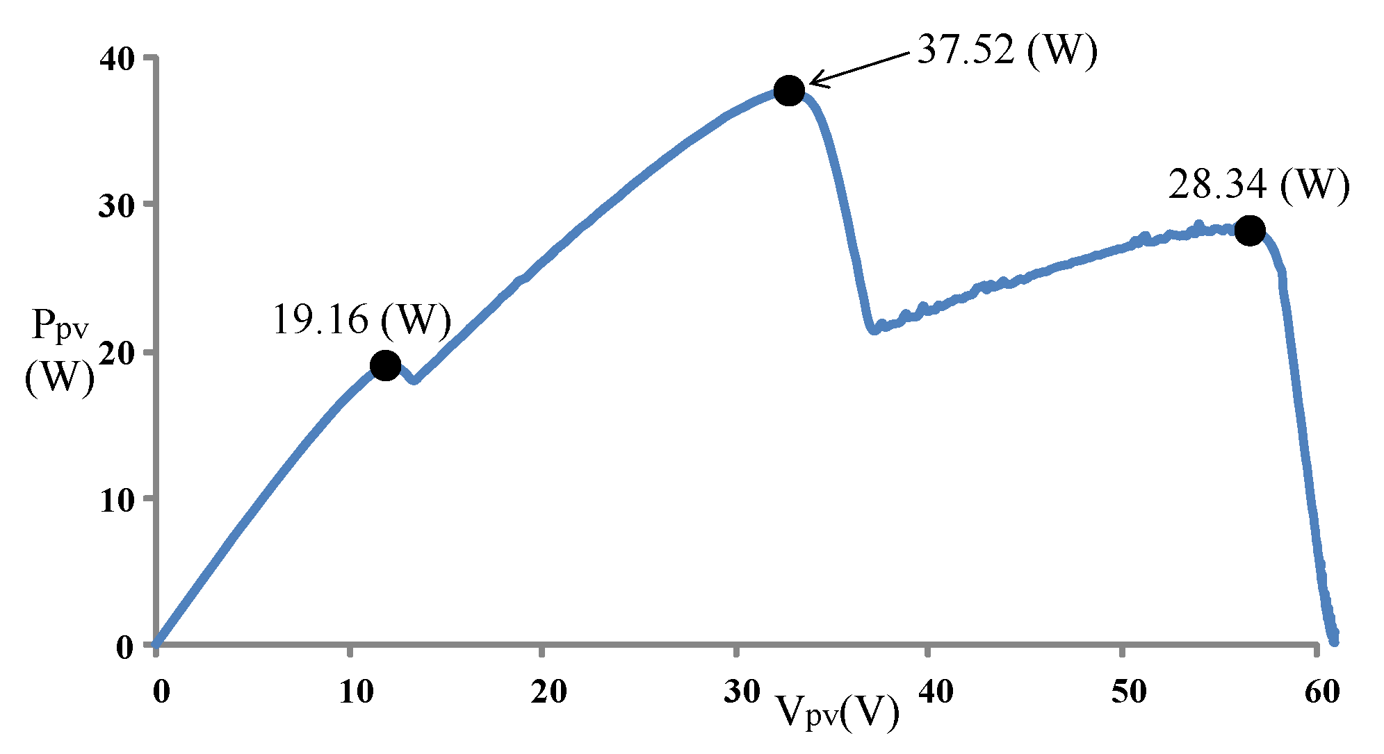
Figure 13.
Maximum power point of Case 2 determined through the conventional PSO algorithm.

Figure 14.
Maximum power point of Case 2 determined through the modified PSO algorithm.

Figure 15.
P–V characteristic curve of Case 3.
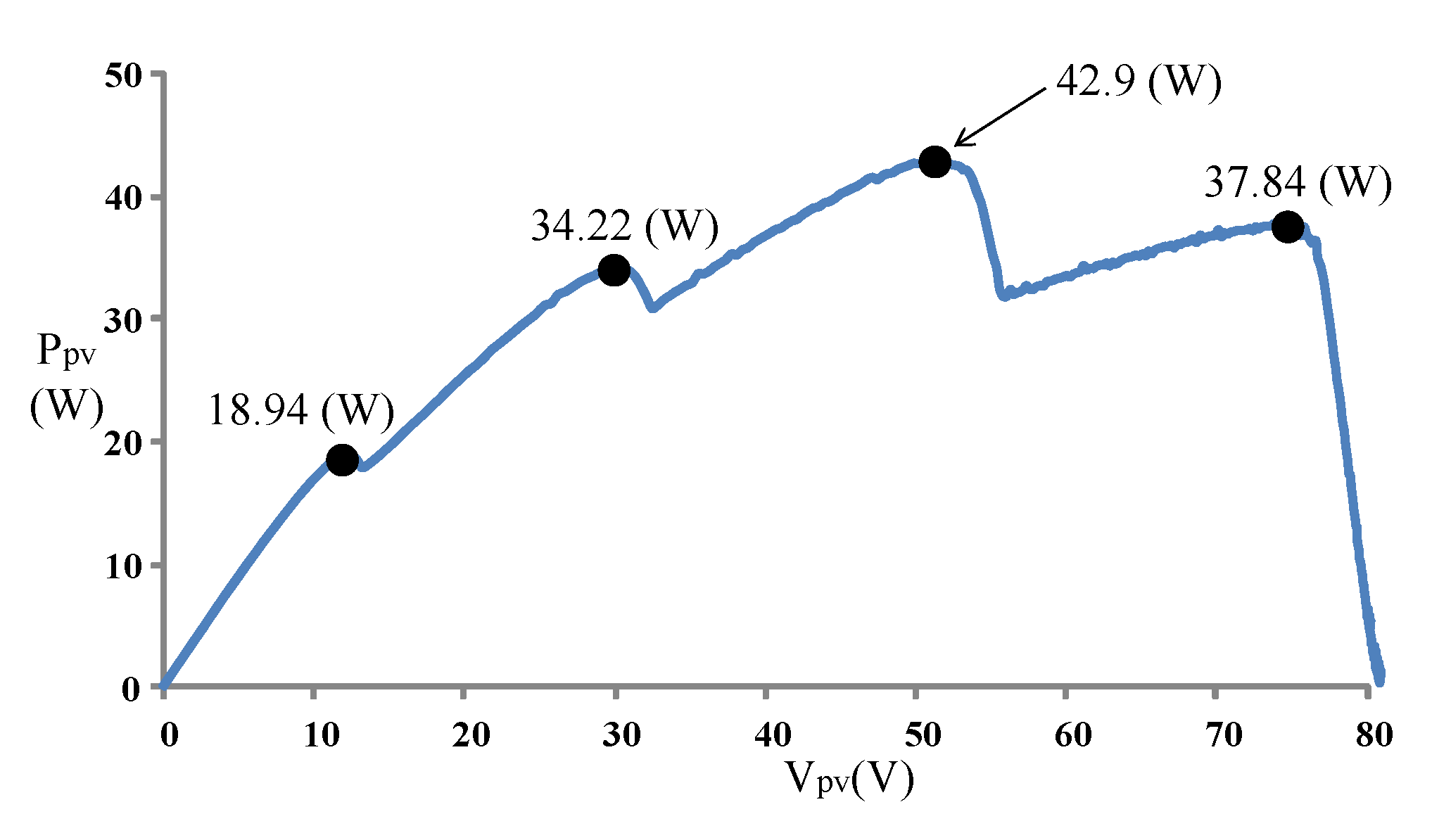
Figure 16.
Maximum power point of Case 3 determined through the conventional PSO algorithm.

Figure 17.
Maximum power point of Case 3 determined through the modified PSO algorithm.

Figure 18.
P–V characteristic curve of Case 4.

Figure 19.
Maximum power point of Case 4 determined through the conventional PSO algorithm.

Figure 20.
Maximum power point of Case 4 determined through the modified PSO algorithm.

Figure 21.
Analysis on the P–V characteristic curve of Case 2.

Figure 22.
Analysis on the P–V characteristic curve of Case 3.


Table 1.
Weighting value adjustment according to the slope and changes in power of the characteristic curve.
Table 1.
Weighting value adjustment according to the slope and changes in power of the characteristic curve.
| Conditions Items | ||
|---|---|---|
| 1 | ||
| 2 | ||
| 3 | ||
| 4 | ||
| 5 | ||
| 6 | ||
| 7 | ||
| 8 | ||
| 9 | ||
| 10 | ||
| 11 |
Table 2.
Parameter configuration of the conventional PSO.
| Parameter | Configured Value |
|---|---|
| Particle number | 4 |
| Iteration number | 100 |
| Weighting (W) | 0.4 |
| Cognition learning factor (C1) | 2 |
| Social learning factor (C2) | 2 |
Table 3.
Parameter configuration of the modified PSO.
| Parameter | Configured Value |
|---|---|
| Particle number | 4 |
| Iteration number | 100 |
| Upper limit of weighting (Wmax) | 0.9 |
| Lower limit of weighting (Wmin) | 0.2 |
| Upper limit of cognition learning factor (C1,max) | 4 |
| Lower limit of cognition learning factor (C1,min) | 2 |
| Upper limit of social learning factor (C2,max) | 4 |
| Lower limit of social learning factor (C2,min) | 2 |
Table 4.
Rated configuration values of the boost converter.
| Component Name | Specifications |
|---|---|
| Inductor L | 1 mH |
| Input capacity Cin | 470 μF/450 V |
| Output capacity Cout | 470 μF/450 V |
| Switching frequency f | 20 kHz |
| Power transistor | IRF460 (500 V/20 A) |
| Diode | DSEP30-12A (1200 V/30 A) |
Table 5.
Specifications of Sanyo HIP2717 module.
| Parameter | Value |
|---|---|
| Rated maximum power () | 27.8 W |
| Current at maximum output power point () | 1.63 A |
| Voltage at maximum output power point () | 17.1 V |
| Short circuit current () | 1.82 A |
| Open circuit voltage () | 21.6 V |
Table 6.
Shading conditions of the four cases.
| Case | Shading Conditions | Number of Peaks in the P–V Curve |
|---|---|---|
| 1 | 2-series 1-parallel: 0% shading + 40% shading | Double peaks |
| 2 | 3-series 1-parallel: 0% shading + 30% shading + 70% shading | Triple peaks |
| 3 | 4-series 1-parallel: 0% shading + 30% shading + 50% shading + 70% shading | Quadruple peaks |
| 4 | 2-series 2-parallel: (25% shading + 0% shading) // (55% shading + 0% shading) | Double peaks |
Note: “+” indicates module connection in series; “//” indicates module connection in parallel.
Table 7.
Comparison of the test results of the four cases.
| Case | Number of Peaks in the P–V Curve | Conventional PSO | Modified PSO | ||
|---|---|---|---|---|---|
| Average Tracking Time | Average Maximum Power | Average Tracking Time | Average Maximum Power | ||
| 1 | Double peaks | 0.96 s | 35.21 W | 0.55 s | 35.32 W |
| 2 | Triple peaks | 1.89 s | 37.08 W | 0.98 s | 37.28 W |
| 3 | Quadruple peaks | Tracking failed | 35.73 W | 1.2 s | 45.55 W |
| 4 | Double peaks | 1.22 s | 64.68 W | 0.67 s | 64.73 W |
© 2018 by the authors. Licensee MDPI, Basel, Switzerland. This article is an open access article distributed under the terms and conditions of the Creative Commons Attribution (CC BY) license (http://creativecommons.org/licenses/by/4.0/).
Share and Cite
MDPI and ACS Style
Chang, L.-Y.; Chung, Y.-N.; Chao, K.-H.; Kao, J.-J. Smart Global Maximum Power Point Tracking Controller of Photovoltaic Module Arrays. Energies 2018, 11, 567. https://doi.org/10.3390/en11030567
AMA Style
Chang L-Y, Chung Y-N, Chao K-H, Kao J-J. Smart Global Maximum Power Point Tracking Controller of Photovoltaic Module Arrays. Energies. 2018; 11(3):567. https://doi.org/10.3390/en11030567
Chicago/Turabian StyleChang, Long-Yi, Yi-Nung Chung, Kuei-Hsiang Chao, and Jia-Jing Kao. 2018. "Smart Global Maximum Power Point Tracking Controller of Photovoltaic Module Arrays" Energies 11, no. 3: 567. https://doi.org/10.3390/en11030567
Note that from the first issue of 2016, this journal uses article numbers instead of page numbers. See further details here.