1. Introduction
Demand side management (DSM) refers to the policy of influencing the energy consumption behaviors of customers by electric power utilities that are beneficial for both sides [
1,
2,
3]. In particular, DSM enables consumers and utilities to actively adjust their electricity demand at any time throughout the day by using the dynamic pricing of electrical energy [
4]. The incentives for the concept of demand response are also enhanced through the relatively recent initiative to incorporate smart meters as part of smart grid developments. The smart grid initiative also enables more efficient operation of the energy grid. Within this new initiative, two-way communication networks are crucial in enabling automation, active and efficient operation and demand response. Hence, DSM is also viewed as a program used by utilities to control energy flow on the consumer side. Consequently, available energy can be used more efficiently without installing new generation and transmission facilities.
Among the myriad benefits of DSM are improving the reliability and security of power systems, easing network congestions, reducing operating, capital and customer costs, and mitigating environmental impacts [
5]. Hence, all existing and future DSM measures will play a major role in reducing system peak loads and in meeting the challenges faced by electric power utilities. Considering this, quantifying the reliability impact of DSM on the power networks is, therefore, important.
The reliability impact of DSM from a generating capacity adequacy assessment viewpoint has been studied and quantified in reference [
5]. A framework was developed to evaluate all possible scenarios for the implementation of interruptible load into demand side management [
6]. Besides that, a project for evaluating the impact of DSM on the transmission and distribution system is described in reference [
7]. Apart from these, the reliability of DSM communication systems has been examined as well [
8]. References [
9,
10,
11,
12] indicate some of the studies that have covered the reliability impacts of DSM on various aspects of a composite power system. All of these studies, however, do not consider the issue of line congestion and the implications for limiting the contributions of DSM. In the case of a specified transmission network capacity, the ability of DSM to ease network congestion is limited by the continuous rise in demand. The dynamic thermal rating (DTR) system offers an effective way to clear line congestion [
13] and it has been widely accepted in the electrical power industry [
14,
15,
16]. Hence, it is also vital to examine the reliability impact of the interactions between DSM and DTR system on a power network.
The characteristics of a DTR system are well detailed in the IEEE 738 standard [
17]. In brief, a DTR system calculates real-time line capacities (
) based on a set of weather conditions and the law of energy conservation such that the convection (
) and radiated (
) heat losses are balanced with the solar (
) and joule (
) heat gains. Mathematically, this is expressed as in (1).
where
and
represent the wind speed, wind angle, air temperature, solar radiation angle, and conductor resistance as a function of its temperature, respectively.
Based on (1), the actual line capacity fluctuates with the weather conditions and this is different from the conventional static thermal rating (STR) operation that fixes line ratings based on very conservative weather assumptions [
18,
19,
20]. Thus, DTRs are usually higher than STRs by 10% to 30% for about 90% of the time, with 50% being possible in windy areas [
21,
22]. Therefore, the DTR system also enables full utilization of the line capacity [
21] and this has assisted the deployment of wind farms worldwide [
20,
23,
24,
25]. Also, references [
19,
26,
27] have quantified the risk and reliability impact of DTR systems on a composite power system. An optimum placing strategy for the DTR sensors on a long overhead transmission line was proposed as well [
18].
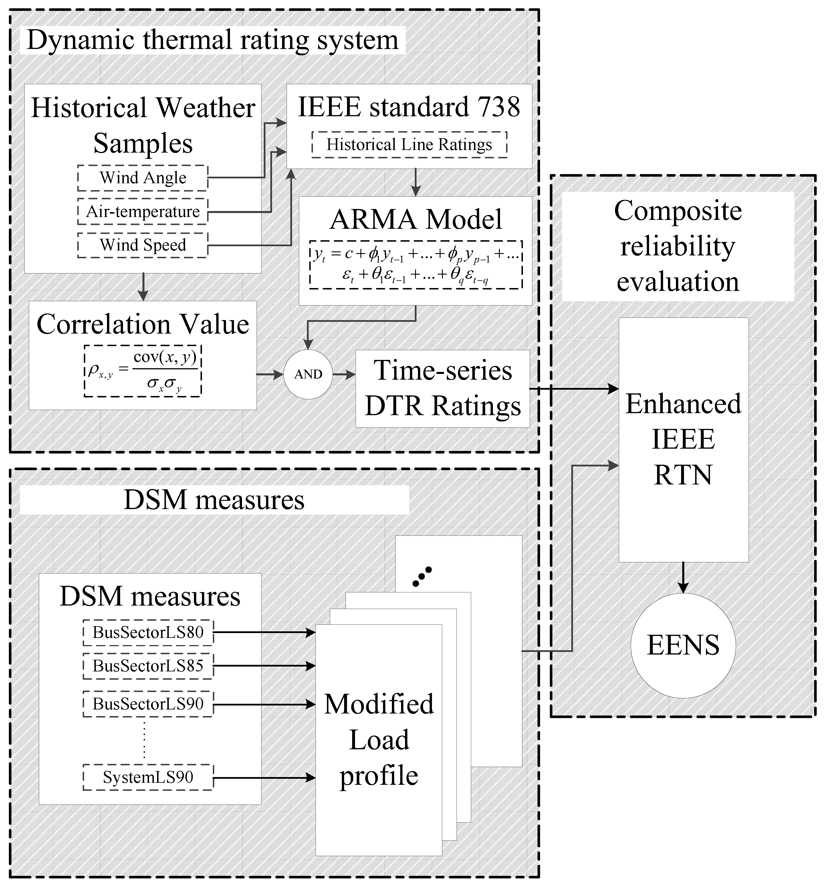
Considering these studies of the DTR system, it seems that there is a lack of research that quantifies the reliability impact of the interactions between DSM and the DTR system on a composite power system. Thus, this paper presents a methodology for the reliability evaluation of a composite power system incorporating DSM and the DTR systems. In this paper, the IEEE reliability test network (RTN) is chosen as the power network for demonstrating the methodology in this paper. The novelty of the methodologies lies in the modelling of DSM, the DTR system, and the combination of both within a single reliability evaluation framework. The proposed modelling of DSM in this paper implements load shifting on the load demand curve from the system, bus and load sector levels. This provides new insight into the reliability impact of DSM as most studies neglect the manipulation of load from the load sector level. The correlation effects of line ratings are considered in the DTR system modelling as the weather that influences line ratings is also correlated. This reflects the actual atmospheric behavior and this is the first time that this has been used in a framework that considers both DSM and the DTR systems. Finally, the modelling of the line ratings was performed using the time series method—an auto regressive moving average (ARMA) model. The ARMA model is more advantageous than the usual probability distribution fitting as distribution functions are not enforced and it can simulate actual trends based on historical data.
2. Composite Reliability Evaluation
In general, the reliability studies of power systems can be performed from three levels [
28]. Each level adds onto the complexity of the previous one, such that level one only analyzes the generation adequacy, level two analyzes generation and transmission network adequacy, and level three analyzes generation, transmission and distribution network adequacy. Level two analysis is known as the composite reliability evaluation and it is performed in this paper.
The Monte Carlo (MC) simulation is the workhorse for conducting power system reliability studies due to its ability to accurately simulate huge numbers of possible power system states [
29]. One of the MCs—the sequential MC (SMC) simulation—is used in this paper as the chronological effects of load managements by DSM and line ratings by the DTR system are considered by the SMC simulation [
28,
29]. In brief, the composite reliability evaluation follows the process below.
Step 1: Initiate the status of all the power system components as the normal up-state. The components refer to the generators and transmission lines.
Step 2: Simulate the duration of residing in the normal and failure states for all the components. The durations of residing in the up- and down-states are governed by the failure and repair rates. These rates are considered to be constant and the inverse transform method [
30] is used to determine the durations. The method mentions that the
ith component state duration
is given as
.
is the uniformly distributed random number in between 0 and 1.
is either the failure or repair rate of the
th component. This step produces cycles of up- and down-states for all the components on an hourly basis.
Step 3: Construct the chronological load model based on the implemented DSM measures (see
Section 4) and calculate the line ratings based on the IEEE 738 standard for the DTR system. Both of these elements are also on an hourly basis.
Step 4: Assess the load loss condition of the power system for each hour by running the direct-current optimal power flow (DCOPF) [
31]. The DCOPF is widely used in the composite reliability analysis as its solution is linear and it has less computational burden [
28,
29].
Step 5: Calculate and update the power system predictive index—expected energy not served (EENS). EENS measures the average amount of energy not served in a year (MWhr/year). Repeat step 2–4 until the coefficient of variation of EENS is less than 5%.
In this paper, the reliability evaluation procedures mentioned above were implemented in MATLAB and the DCOPF was executed using MATPOWER 5.0 [
31]. Hereinafter, the term “composite reliability evaluation” refers to the procedures and methods described in this section.
3. Test System Data
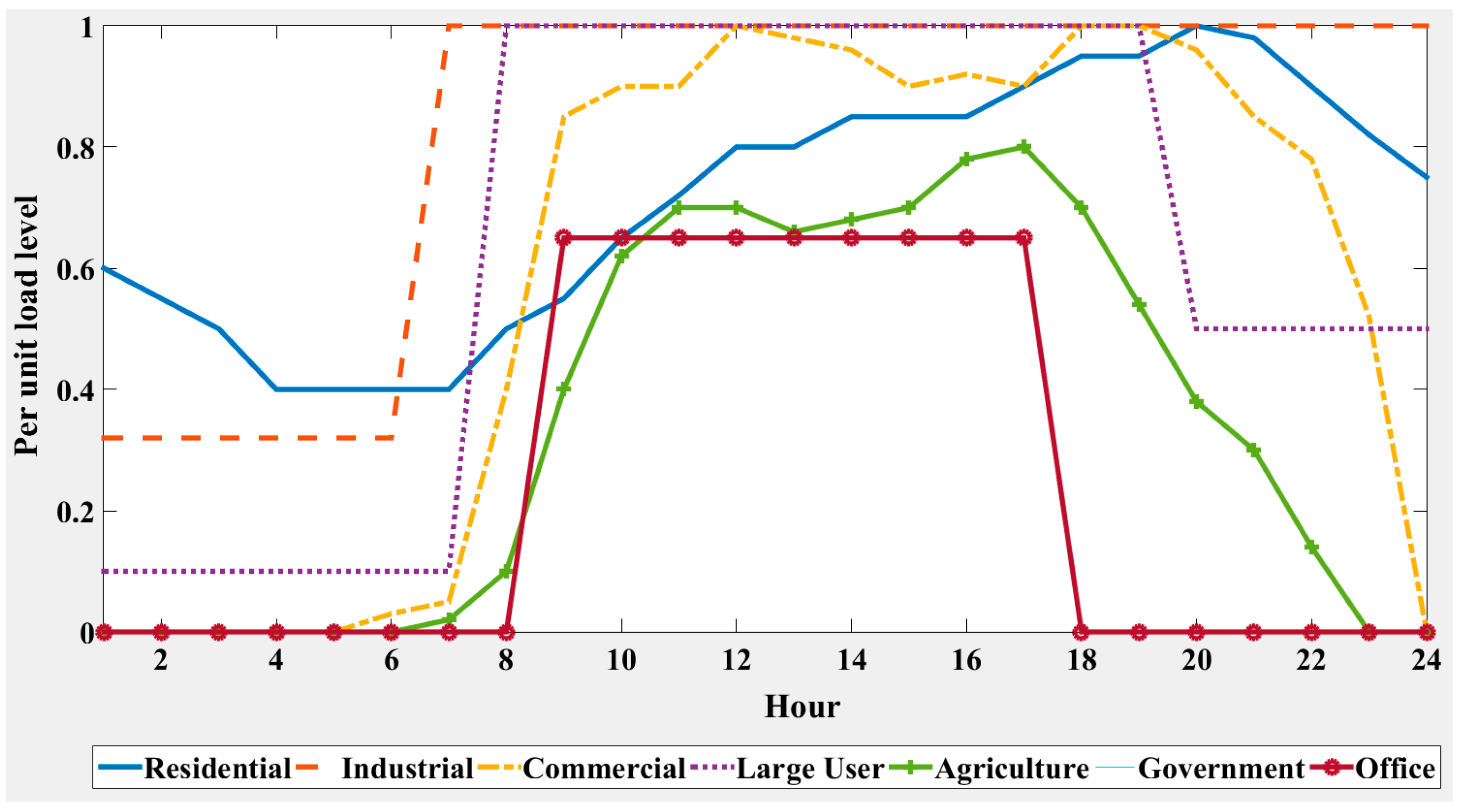
The original IEEE RTN [
32] is a 24-bus network with 33 transmission lines, 32 generating units, 10 generator buses and 17 load buses. It has a total installed generating capacity of 3405 MW and a total system peak load of 2850 MW. This specified total system demand, however, does not indicate the variation of individual bus loads during the period concerned. A more comprehensive version of the system load would recognize that individual buses have different load curves and they are a composition of various load classes which all have unique curves. Hence, this necessitates the development of a load model starting from the perspective of the load sectors at each bus and a new collective hourly load curve for the system can then be developed. This information is, however, generally rare and for this reason, this paper adopts the load sector curves as presented in [
5,
33]. The 24-h load curves for all the load sectors are presented in
Figure 1. In addition, the customer compositions at each load point are specified as well and they are as shown in
Table 1 [
33].
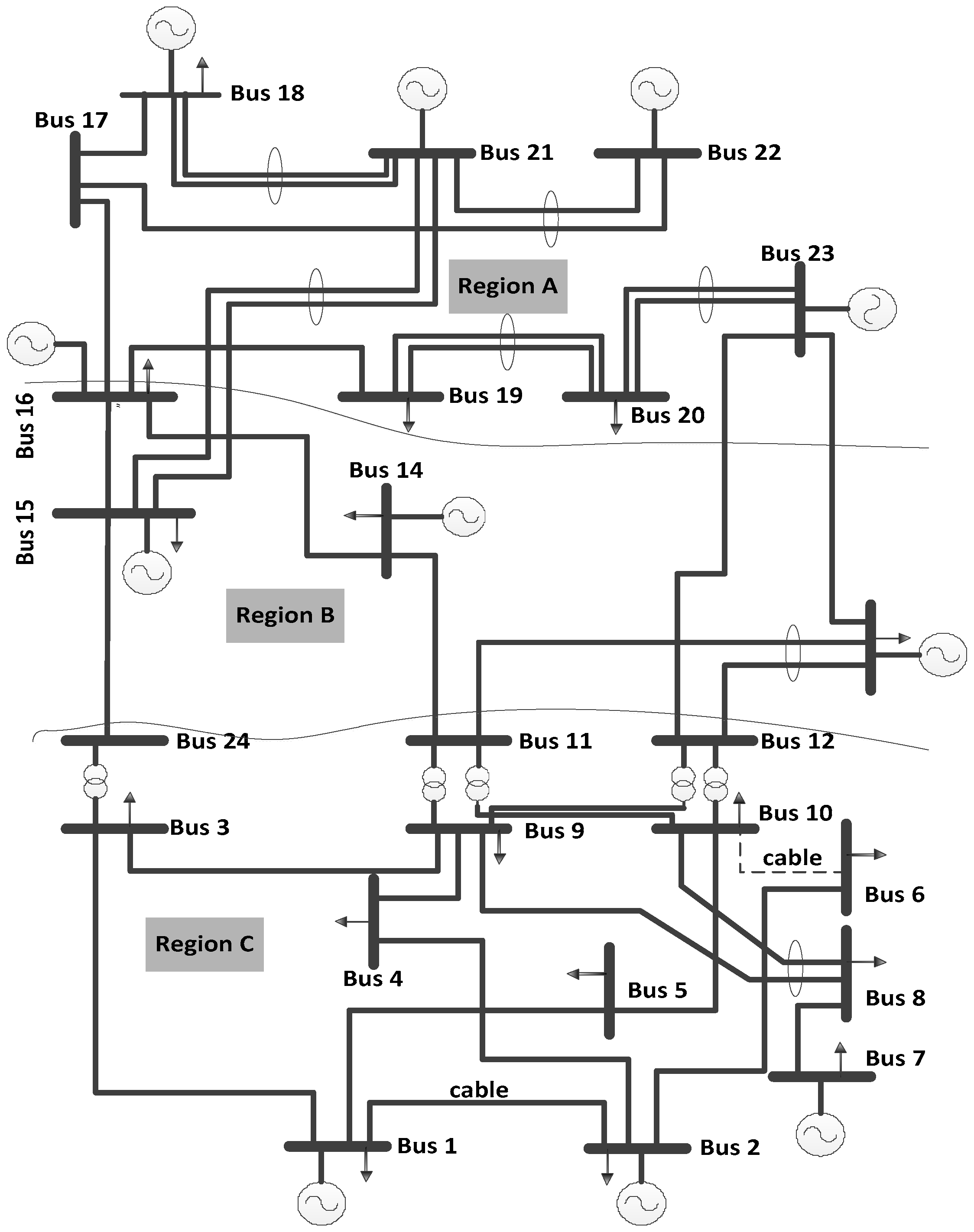
The enhanced RTN is also divided into three regions—A, B and C—as shown in
Figure 2. Region A is considered to be further away from region C than its neighboring region B and similar logic applies to the other two regions. Each transmission line in the enhanced RTN is also equipped with a DTR system. Note that the lines with a common tower or right-of-way share a DTR system due to their proximity.
4. DSM Measures
The load shifting initiatives of the DSM in this paper transfer all the energy not supplied during the on-peak hours to the off-peak hours according to the calculation as shown in (2) [
6].
where
L(t) is the original load model; is the modified load model; P is the pre-specified peak; Ω is the set of on-peak hours when the demand is reduced; is the set of off-peak hours when the demand is recovered; and N is the number of off-peak hours in .
The energy reduced during the on-peak hours is shifted to the immediate off-peak hours, whereby these hours are determined based on the pre-specified peak and valley load values, respectively. The energy added during the off-peak hours is limited to the maximum of the pre-specified peak. All the load shifting initiatives performed in this paper are mentioned in
Table 2. The table shows that 3 pre-specified peak values, 80%, 85% and 90%, were considered and all of them share the same pre-specified valley values.
The BusSectorLS measures apply load shifting to each load sector individually and the modified load profiles are summed to produce the bus loads which are then further summed to form the system load. The BusLS measures apply load shifting to the load of each bus and the modified load profiles of the buses are summed to form the system load. Finally, the SystemLS measures perform load shifting directly on the system load profile.
For the purpose of illustration, the system load profiles of all the DSM measures performed on each load sector (BusSectorLS) are shown in
Figure 3. The figure shows that BusSectorLS80 has, among them, the flattest curve as it clipped-off the most load to fill in its valleys. BusSectorLS85 and BusSectorLS90, have load curves that are similar to the original load shape. This discussions for
Figure 3 are also applicable for all the other DSM measures and they are not shown in this paper due to space limitations.
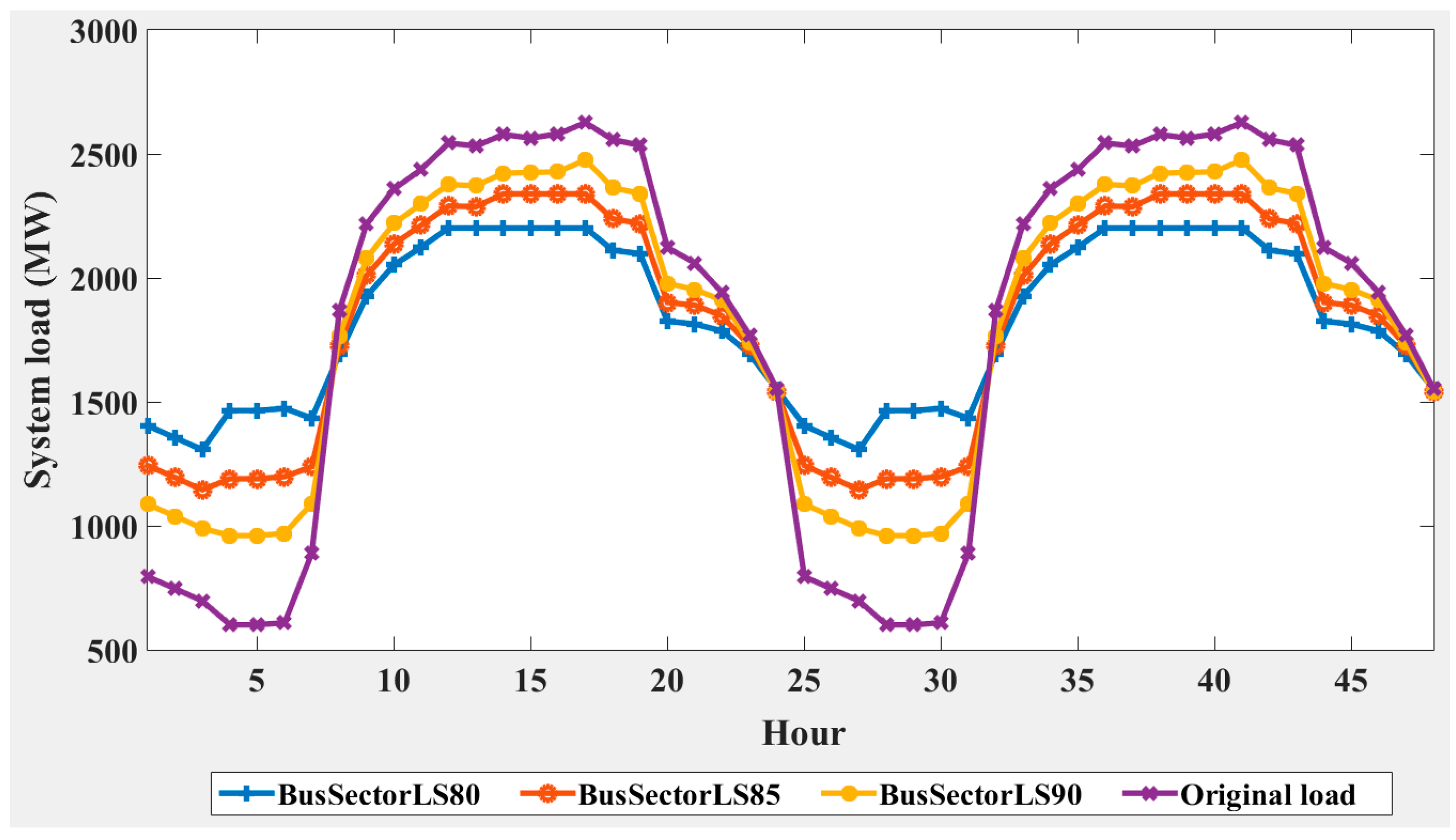
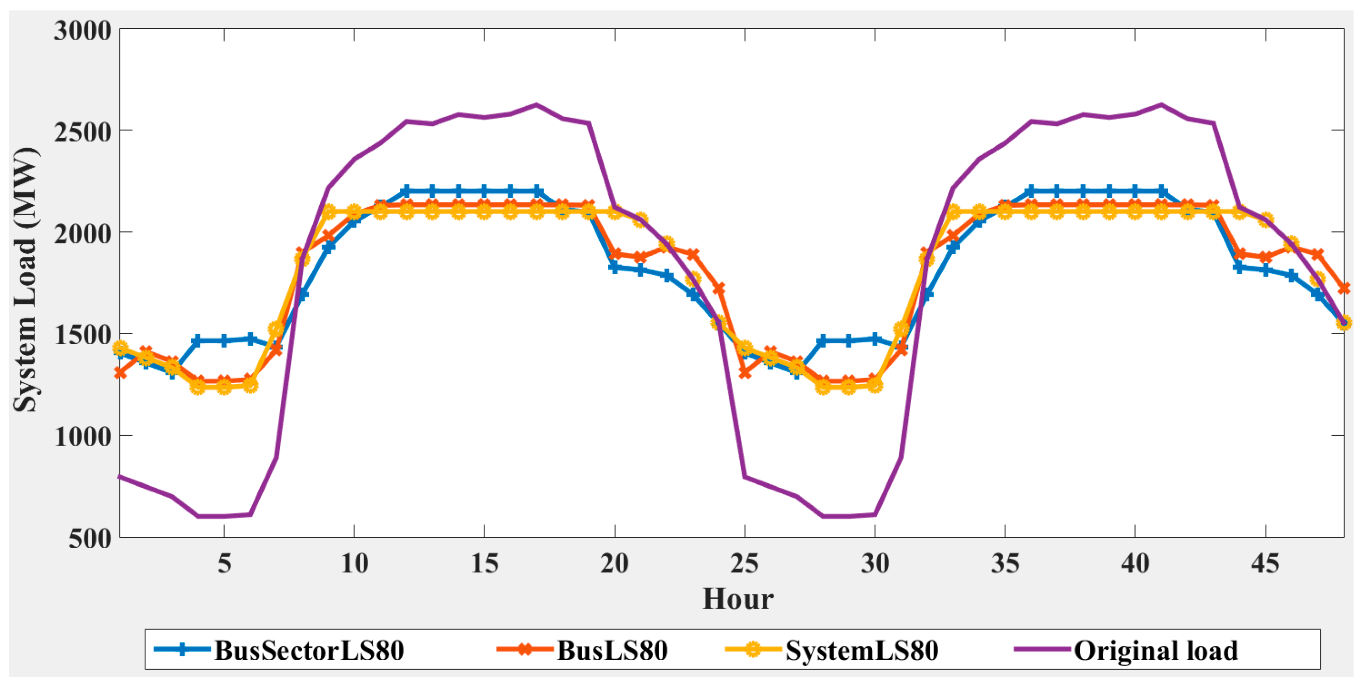
Then, the comparison of the 48-h system load profiles of all the DSM measures using the 80% pre-specified peak are shown in
Figure 4. The figure shows that BusLS80 and SystemLS80 have similar load shapes but the BusLS80 load profile has a slightly shorter peak duration. In terms of their valleys, they are both very similar to each other. BusSectorLS80, however, is different than the other two DSM measures mentioned previously. It has larger peak and valley values and it also has steeper rise and fall times in its load curve. As a result, the BusSectorLS80 has a shorter duration of peak loads as well.
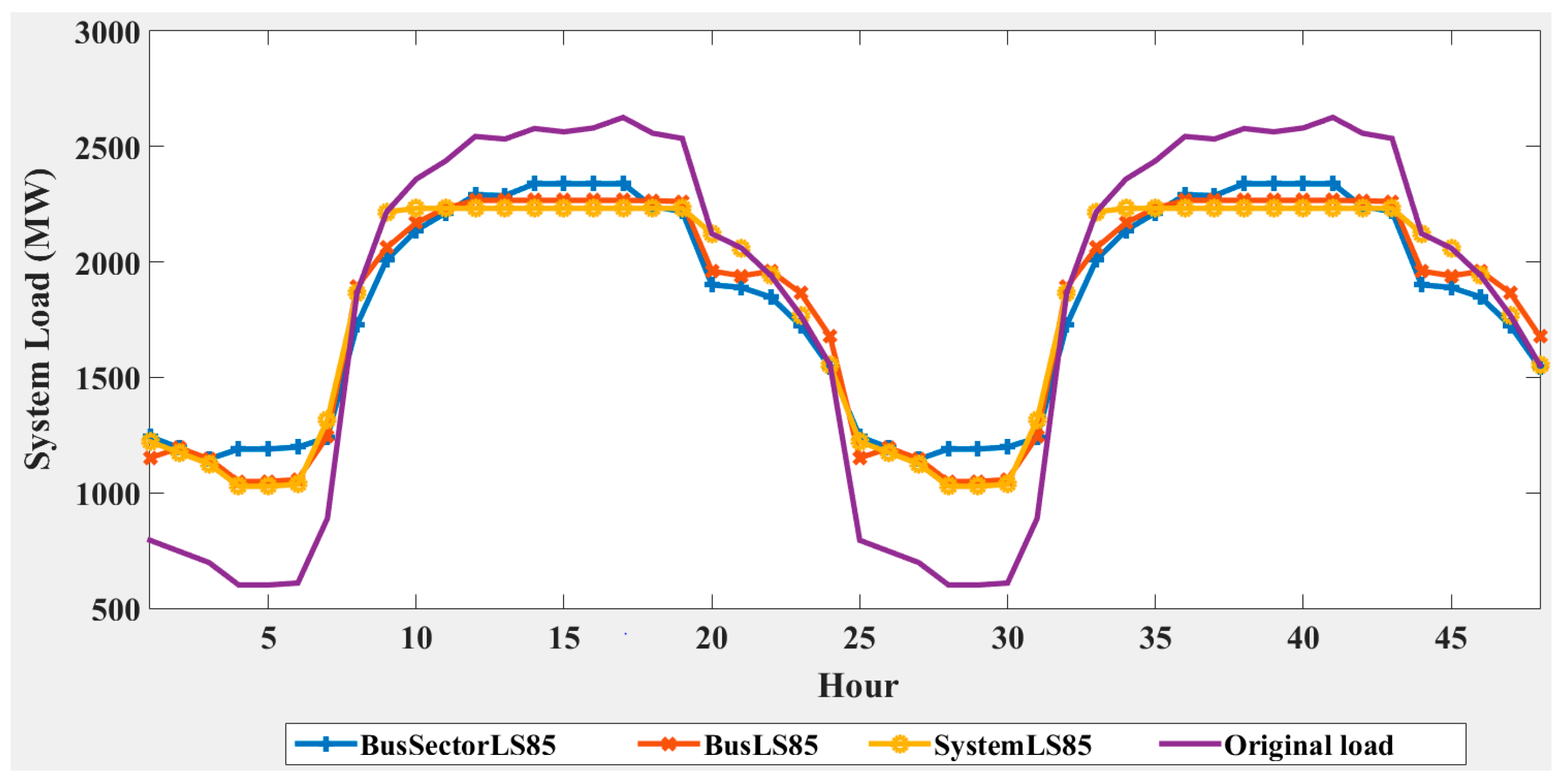
Similar comparisons were also performed for all the DSM measures using the 85% pre-specified peak and they are as shown in
Figure 5. The results show similar patterns as in
Figure 4 but there are slight variations in the magnitude of the curves. The results in
Figure 5 show that the BusLS85 load profile has a slightly shorter peak duration than SystemLS85 and both measures have comparable valley curves. As for BusSectorLS85, it shows steep rise and fall times in its load curve, which lead to a shorter duration of peak loads—a characteristic similar to BusSectorLS80.
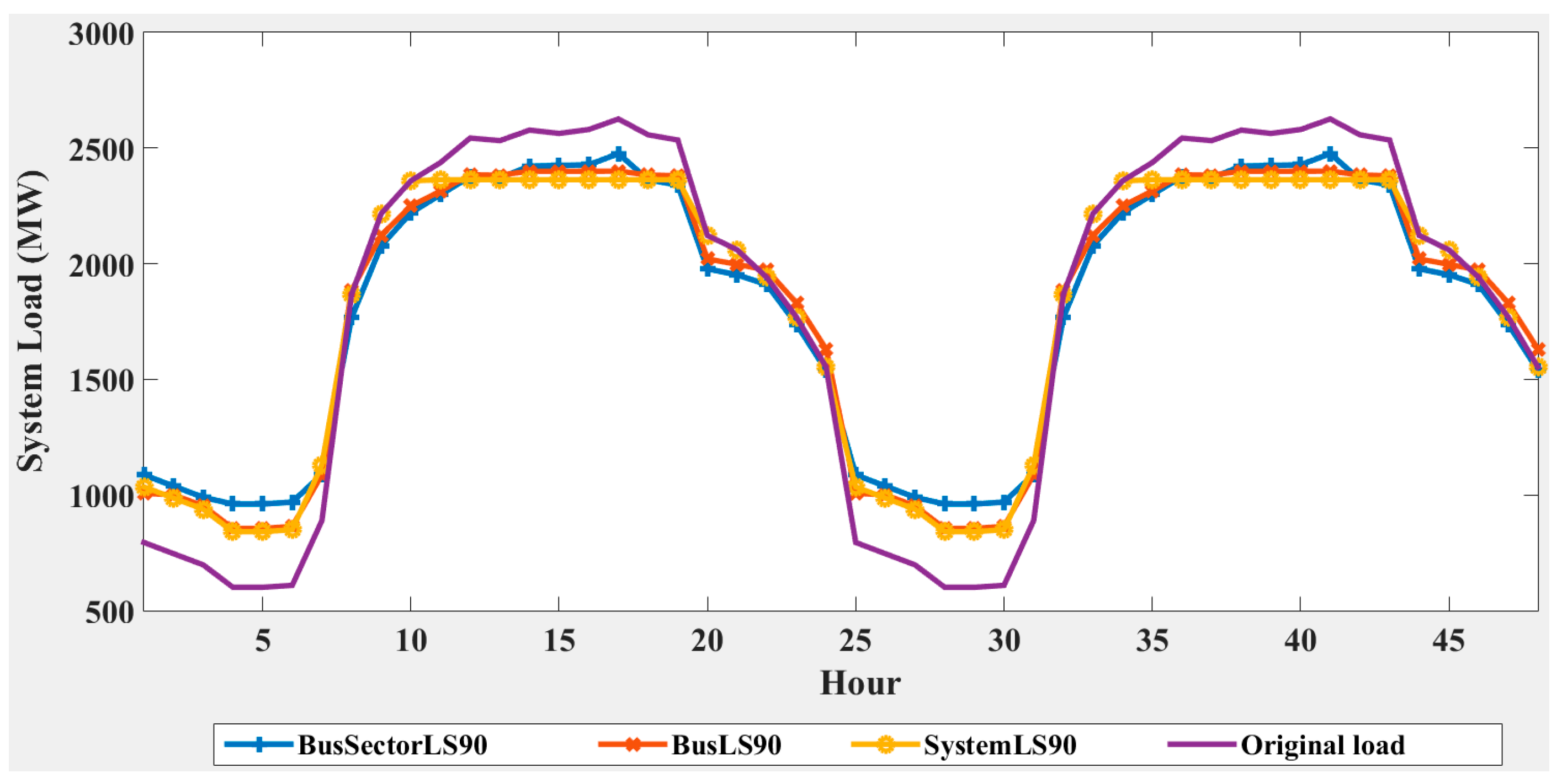
Finally, the comparisons for all the DSM measures using the 90% pre-specified peak were performed and they are as shown in
Figure 6. All the DSM measures under this policy have load curves that are almost similar to each other. Despite that, the load patterns in
Figure 4 and
Figure 5 remain in
Figure 6. In other words, the differences between BusLS90 and SystemLS90 are similar to the differences between BusLS80 (or 85) and SystemLS80 (or 85). The BusSectorLS90, similarly with BusSectorLS80 and BusSectorLS85, has a load curve with steep rise and fall times, resulting in a shorter duration of peak loads.
5. DTR System
Twenty-one transmission corridors were identified in the enhanced IEEE RTN after considering the lines with a common tower or right-of-way. Based on this information, 21 DTR systems are implemented in the enhanced IEEE RTN and it is further considered that each of the DTR system is affected by a different weather profile. Hence, 21 sets of weather data are required for the modelling of the DTR systems. In order to do that, 21 sets of 20 years of historical weather data with the time resolution of an hour was sampled from the British Atmospheric Data Center (BADC) website [
34]. These weather data were used to calculate the historical line ratings of each of the transmission corridor by following the DTR system theory in (1). In addition, all of the weather data require by the DTR systems that are residing in the same region of the enhanced IEEE RTN were sampled from the locations that are no further than 50 km apart. The weather data in between the regions, however, were sampled from locations that are separated by about 100 km.
Then, according to [
35], the propagation of the historical weather data, and hence the line ratings, follow a trend and they are not completely random. Considering this, the historical line ratings are more suitably modelled using the auto-regressive and moving-average (ARMA) model instead of the commonplace distribution-fitting method. Generally, an ARMA model with
-order auto-regressive and
-order moving-average
components is as shown in (3).
where
yt is the future conditional mean value;
is the past observed values;
is the auto-regressive constant;
is the moving-average constant;
—
is the normally and independently distributed random white noise with zero mean and
variance; and
is past random innovation values.
The ARMA (
) process in (3) shows that a future conditional mean value of line ratings (
is affected by its past observed values and past random innovation values. Hence, (3) also demonstrates that the ARMA model can produce realistic line rating values during the SMC simulation process while preserving the line rating values of actual data trends [
35].
In addition to the ARMA modelling, the correlations among the ARMA models need to be considered as well. This is because the calculated historical line ratings are correlated in the same way as their weather data. In order to do that, the correlations among the line ratings were first determined using the Pearson’s product-moment as shown in (4).
where
is the correlations between vector
and
;
is the covariance between vector
and
; and
is the standard deviation of a vector.
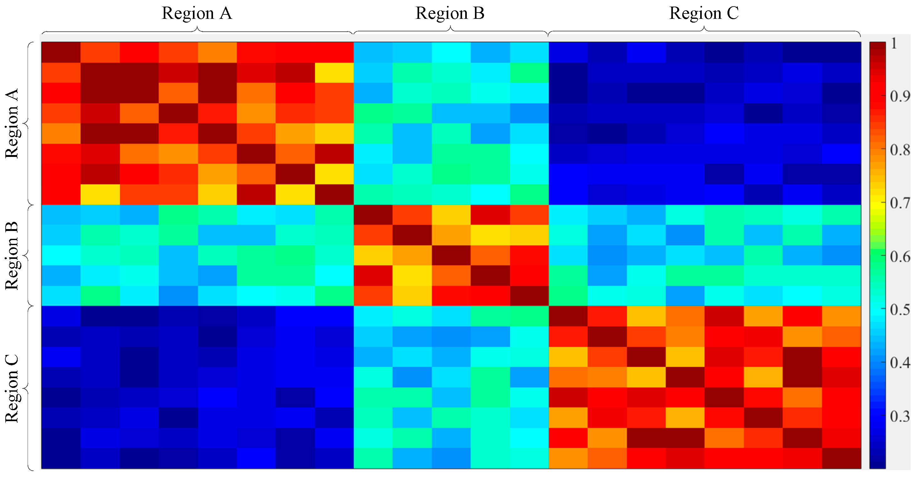
The correlations among the line ratings as a result of the application of (4) is shown as a heat map in
Figure 7. The results show that the correlations among the line ratings from the same region of the enhanced IEEE RTN is strong. The strength of the correlation, however, reduces when the line ratings from different regions are compared. In general, the strength of the correlation is inversely proportional to the distance in between the line ratings. For example, region A has a weaker correlation with region C than with region B. Taking this into account, it is vital that the correlations among the ARMA models are considered during the simulations of their line ratings.
As mentioned earlier in (3), the simulation of an ARMA model is dependent on its random innovations that are sampled from an independent normal distribution. Such simulations of all the ARMA models will produce line rating vectors that are independent of each other. A common multivariate normal distribution, however, that considers the correlations among all the ARMA models will produce line rating vectors that are also correlated in the same way. Hence, in this paper, the common multivariate normal distribution is formed by generalizing the univariate normal distribution to 21 variables (21 sets of line ratings). This process is mathematically described by (5).
where
is the vector of correlated innovations;
x is the vector of random innovations;
p is the number of the ARMA model;
μ— is the mean vector of random innovations for all the considered ARMA models; and Σ—
is the symmetric covariance matrix for all the considered ARMA models. It can be obtained by rearranging (4) and its diagonal elements represent variances.
Considering both the DSM model in
Section 4 and the DTR system model in this section, an overview of the proposed methodology is presented and it is as shown in
Figure 8. The figure shows that the proposed methodology is divided into three main parts—the DSM measures, the DTR system and the composite reliability evaluation. For the DTR system, historical weather data was used to determine historical line ratings based on the IEEE 738 standard. These line ratings are then modelled with ARMA models. The ARMA models together with their correlation information derived from their respective weather data, are used to simulate line ratings for each transmission corridor and these ratings are updated into the enhanced IEEE RTN. At the same time, in measuring the DSM, the enhanced load model is manipulated according to the selected DSM measure and the resultant load profile is also updated into the IEEE RTN. Finally, a composite reliability evaluation is performed on the updated enhanced IEEE RTN and the EENS index value is recorded to quantify the reliability performance.
6. Results and Discussions
6.1. Effects of DSM Measures
All the DSM measures in
Table 3 were implemented together with the described DTR system in the enhanced IEEE RTN. In this part of the studies, the actual correlations among the DTR systems are considered and the loading level was incrementally increased by 20% up to twice the original loading level. Due to space limitations, only the EENS values for all the DSM measures at the original and the maximum loading levels are reported and they are shown in
Table 3.
The results indicate that the SystemLS measures have the worst reliability performance compared to the other DSM measures. In contrast, the BusSectorLS measures have the best reliability performance regardless of the loading levels, and hence, they also have the lowest EENS values. Nonetheless, the BusLS measures are just slightly worse than the BusSectorLS measures. The reason for these is that the SystemLS measures have longer peak durations than the other measures for all levels of the pre-specified peak load (
Figure 4,
Figure 5 and
Figure 6), which leads to a higher probability of loss of load under this group of DSM measures. Besides that, when the BusSectorLS measures are implemented, the load duration curve decreases much faster from the peak load than the SystemLS measures, and thus, improving their EENS values and further widening the gap between the EENS values of these two groups of DSM measures.
Moreover, it is also noticeable that the differences between the EENS of BusSectorLS, BusLS and SystemLS measures are larger when the pre-specified peak load is high and this effect is amplified with increasing load level. For example, the EENS of BusSectorLS90 is lower than BusLS90 and SystemLS90 by 18 MWhr/year and 293 MWhr/year, respectively, at the original load level. These values increase to 12,928 MWhr/year and 18,712 MWhr/year at twice the original load level. These results show that the reliability performance of the IEEE RTN benefit the most when the DSM measures are implemented on the load sector level. This is because when load sectors are considered individually, there are more opportunities for load shifting.
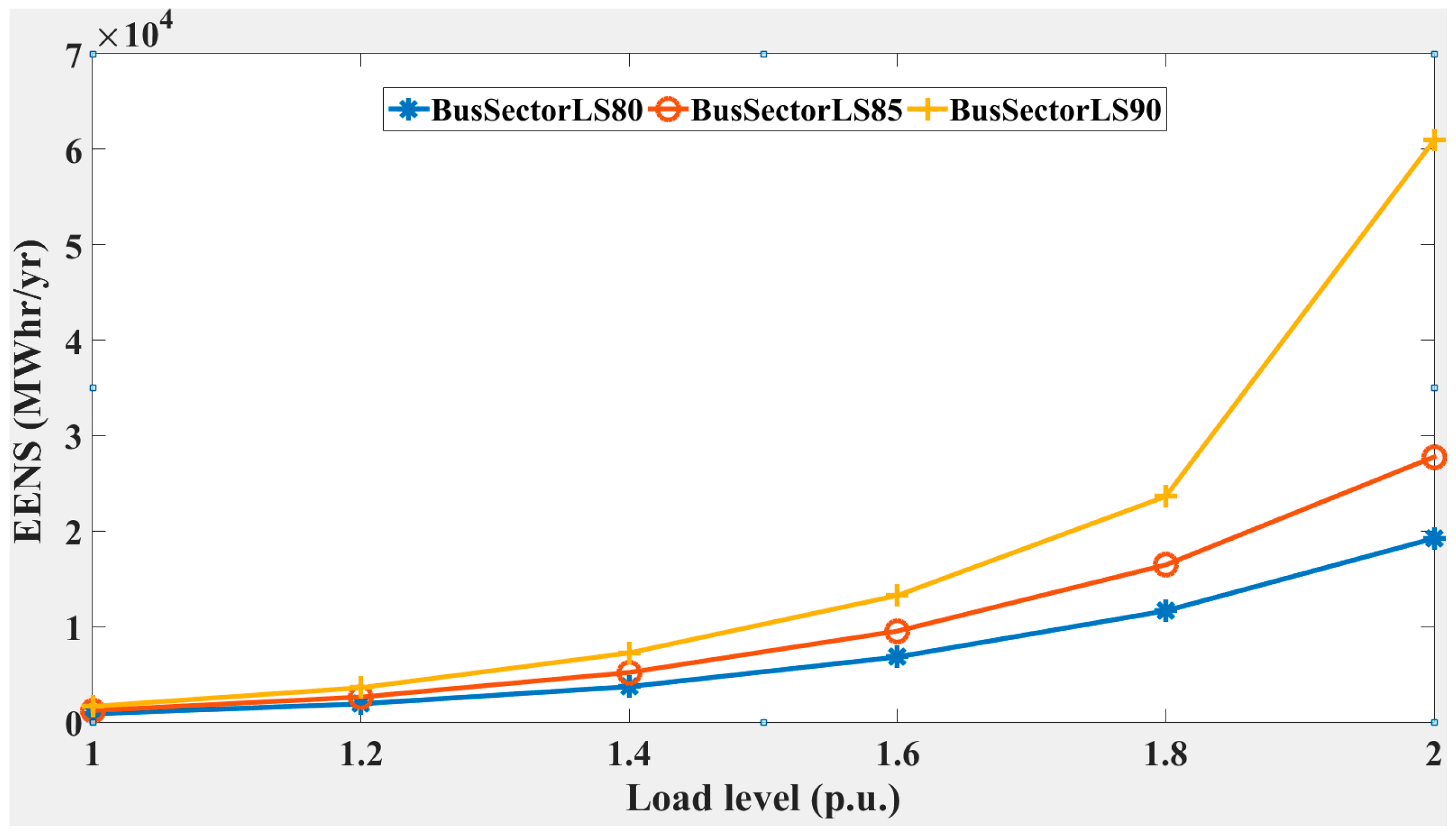
When the DSM measures are compared within a group, the DSM measure with a lower pre-specified peak load has a better (lower) EENS value. For example, BusSectorLS80 performs better than BusSectorLS85 and BusSectorLS90. This effect is highlighted as the load level increases and this is shown in
Figure 9. The reason for this is that BusSectorLS80 performs more load shifting than the other BusSectorLS measures. When the pre-specified peak load is lower, for example 80%, a higher amount of load is clipped-off as compared to 85% or 90%. A similar logic also applies for the other groups of DSM measures but only the BusSectorLS measures are plotted in
Figure 9 because they have the best reliability performance.
6.2. Effects of DTR System Correlations
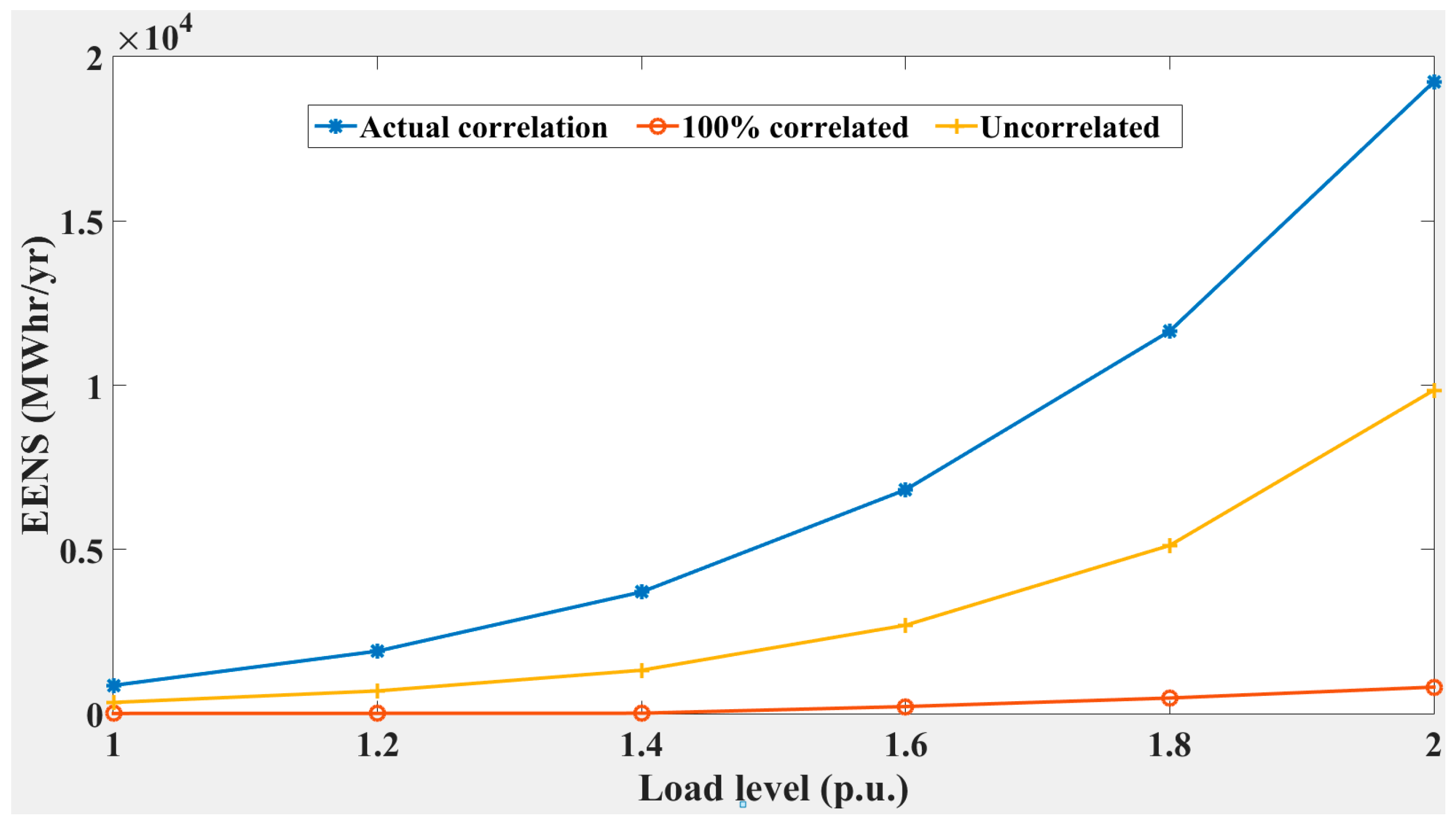
In this section, the correlation effect of the DTR system on the reliability performance of the DSM measures are investigated. In particular, the BusSectorLS80 was selected in this investigation as it has the best reliability performance among all the DSM measures as proven in the previous section. The result of this study is given in
Figure 10. In the figure, the term “Actual correlation” means the real correlations among the DTR system line ratings are considered during the implementation of BusSectorLS80. The term “100% correlated” means that all the DTR system line ratings are considered to be fully correlated. This scenario represents the opposite extreme of the case when the correlations of the DTR system are not considered at all, which is represented by the term “Uncorrelated”.
In
Figure 10, it can be seen that the EENS values are the lowest under the “100% correlated” scenario and this is due to the strong influence of the desirable high line ratings on the undesirable low line ratings. Under this condition, the average simulated line rating values increase dramatically and this allows higher flow of line current to meet more demand. As a result, this scenario also gives an unrealistic, underestimation of the true EENS index value.
In the “Uncorrelated” scenario, however, the correlations among the line ratings are not considered—the DTR systems are independent of each other. Hence, the simulation of the DTR system with low line ratings remain low and they are not affected by the simulation of the DTR system with high line ratings. As a result, this scenario has higher EENS values than the “100% correlated” scenario. Despite this, its reliability performance is an underestimation of the true reliability performance given by the “Actual correlation” case.
The results of this section show that the correlations among the DTR system are an important factor to be considered when studying the joint reliability impact of DSM and DTR systems on power networks.
6.3. Effects of the DTR System
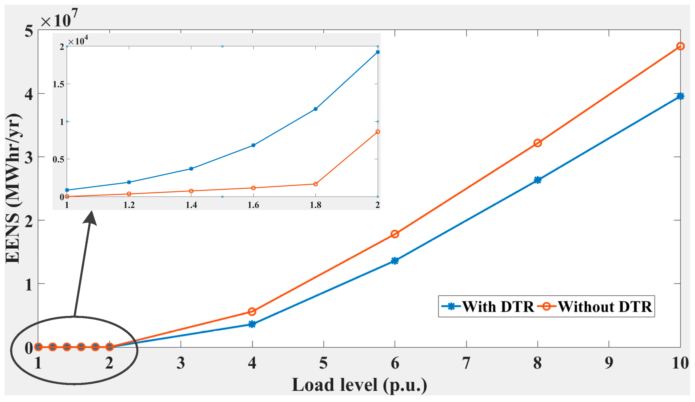
In this section, the impact of the DTR system on the reliability performance of BusSectorLS80 is investigated and the results are shown in
Figure 11. In the figure, the terms “With DTR” and “Without DTR” refer to the conditions where the BusSectorLS80 was implemented with, and without the application of the DTR system on the transmission network, respectively.
The results show that when the load level is less than 2, the EENS values of BusSectorLS80 with the DTR system is higher than without the DTR system. The reason is that at these load levels, BusSectorLS80 alone is sufficient to mitigate load losses. As the application of the DTR system will introduce low line ratings in some undesirable weather conditions and leads to line congestion, the probability of load loss will increase during these load levels, when BusSectorLS80 was implemented with the DTR system.
However, as the load level continues to rise beyond twice the original level, the EENS of BusSectorLS80 without the DTR system rises above the EENS of BusSectorLS80 with the DTR system. Although there are periods of low line ratings due to the DTR system, the reliability benefit of the high line rating periods far outweighs the drop in the reliability due to low line rating periods. Besides that, BusSectorLS80 alone at these high load levels is not effective in mitigating load losses as its contribution is limited by static thermal ratings if no DTR system is implemented.
7. Conclusions
In this paper, the system and bus loads are divided into 7 sector loads. The analyses in this paper show that the system load and the bus load do not change significantly when a DSM measure is applied to them as they are a composition of sector loads. The load shape, however, changes significantly when a DSM measure is applied to each individual sector load. As a result, the summation of all these sectors causes a huge change to the resulting system or bus load.
As also noted in this paper, a methodology for a joint evaluation of the reliability impact of DSM and a DTR system on a composite power network was proposed. The results of this paper show that the reliability impact of DSM is different when the DSM is applied to system load, bus loads and all sector loads. Generally, the DSM implemented on sector load benefits the reliability of the IEEE RTN, the most. The effects of the DTR system correlations was examined as well. This study demonstrates that the inaccurate representation of the correlation values can lead to underestimation and an incorrect reliability evaluation. Finally, the study also shows that at low load levels, DSM improves the reliability of the RTN more if the DTR system is not implemented. At high load levels, however, the reliability performance of the DSM is better if the DTR system is implemented. The reader, however, should note that this conclusion was drawn based on the adopted load curves in
Figure 1. Although the numerical results will change with different load curves, the methodology presented in this paper is still applicable.
The work presented in this paper can be extended to incorporate renewable energy sources, such as wind power, and energy storage. The reason is that the wind that affects line ratings also changes the power outputs of wind turbines. It has been recognized that wind farm operations benefit from line rating enhancement by DTR systems. However, the addition of DSM into this mix has not been examined and its impacts have not been quantified. Moreover, the presence of DSM might decrease the need for the DTR systems as peak load demands have been reduced. The application of energy storage and DTR systems would be another worthwhile venture because energy storage is used to store excess wind energy when there is excessive wind power output or when the line capacity is congested. This interaction will change with the implementation of the DTR systems as line capacity is upgraded. The effect will become more complicated as DSM is introduced into the equation.

 ,
, 


