Ensemble-Based Data Assimilation in Reservoir Characterization: A Review


1
E&P Business Division, SK Innovation, Seoul 03188, Korea
2
Petroleum and Marine Research Division, Korea Institute of Geoscience and Mineral Resources, Daejeon 34132, Korea
3
Department of Energy and Resources Engineering, Kangwon National University, Chuncheon 24341, Kangwon, Korea
4
Department of Energy Systems Engineering, Seoul National University, Seoul 03080, Korea
*
Author to whom correspondence should be addressed.
Energies 2018, 11(2), 445; https://doi.org/10.3390/en11020445
Submission received: 9 January 2018
/
Revised: 7 February 2018
/
Accepted: 9 February 2018
/
Published: 17 February 2018
(This article belongs to the Section L: Energy Sources)
Abstract
:This paper presents a review of ensemble-based data assimilation for strongly nonlinear problems on the characterization of heterogeneous reservoirs with different production histories. It concentrates on ensemble Kalman filter (EnKF) and ensemble smoother (ES) as representative frameworks, discusses their pros and cons, and investigates recent progress to overcome their drawbacks. The typical weaknesses of ensemble-based methods are non-Gaussian parameters, improper prior ensembles and finite population size. Three categorized approaches, to mitigate these limitations, are reviewed with recent accomplishments; improvement of Kalman gains, add-on of transformation functions, and independent evaluation of observed data. The data assimilation in heterogeneous reservoirs, applying the improved ensemble methods, is discussed on predicting unknown dynamic data in reservoir characterization.
1. Introduction
Data assimilation, as a methodology for integrating various kinds of data, is defined as an analysis technique in which the observed information is accumulated into the model state, by taking advantage of consistency constraints with laws of time evolution and physical properties. The technique uses measured data and the theoretical information of the system to improve knowledge of the past, present, or future system states. The framework of typical data assimilation is a recursive method by updating the model state, i.e., ensembles, since the new estimate is a function of the previous estimate, and thereby it updates the ensembles to match the observed data [1,2].
Data assimilation techniques can be categorized as variational schemes, statistical schemes, or hybrid schemes [3,4]. The variational schemes are based on least squares estimation for maximum likelihood, while the statistical methods estimate minimum variance for least uncertainty. The variational schemes, originating from optimal control theory, minimize some cost function that expresses the distance between observations and corresponding model values, using the model equations as constraints [5]. Typical variational methods are 3D-Var, 4D-Var [6], and Nudging [7]. The statistical schemes emanate from estimation theory, and use the error covariances of the observations and of the model predictions to find the most likely linear combination of the two [5]. The classic approach is the Kalman filter for linear problems, whereby for strongly nonlinear problems, it is extended to the ensemble Kalman filter (EnKF), ensemble smoother (ES), ensemble Kalman smoother (EnKS), and other variants. Lastly, the hybrid method integrates both of the above schemes to combine their different strengths. Ensemble of data assimilation (EDA), NDEnVAR [8] and Iterative Ensemble Kalman Smoother (IEnKS) [9] are categorized as hybrid schemes.
Since the real reservoirs are very uncertain, data assimilations in reservoir characterization have focused on uncertainty quantification and reliable data integration with available dynamic and static datasets. Thus, in the field of reservoir engineering, statistical schemes, such as EnKF and ES, have been actively researched. They assume the initial state of the reservoir (pressures, temperatures, and saturations) and the joint probability of reservoir parameters are known, and that the future state can be generated by updating the current and past states [10]. The dynamic data consisting of the assimilation objectives are continuously updated, and thereby reliable revision of plausible or optimal reservoir models is still challengeable. As the amount of data increase, the more reliable reservoir characterization has demanded intensive data integration to match all available spatiotemporal data, as well as newly updated data. However, the different-scaled data, high nonlinearity, and limited available information cause difficulties for more reliable data assimilations with mathematical clearness, and also for improved predictions of unknown properties.
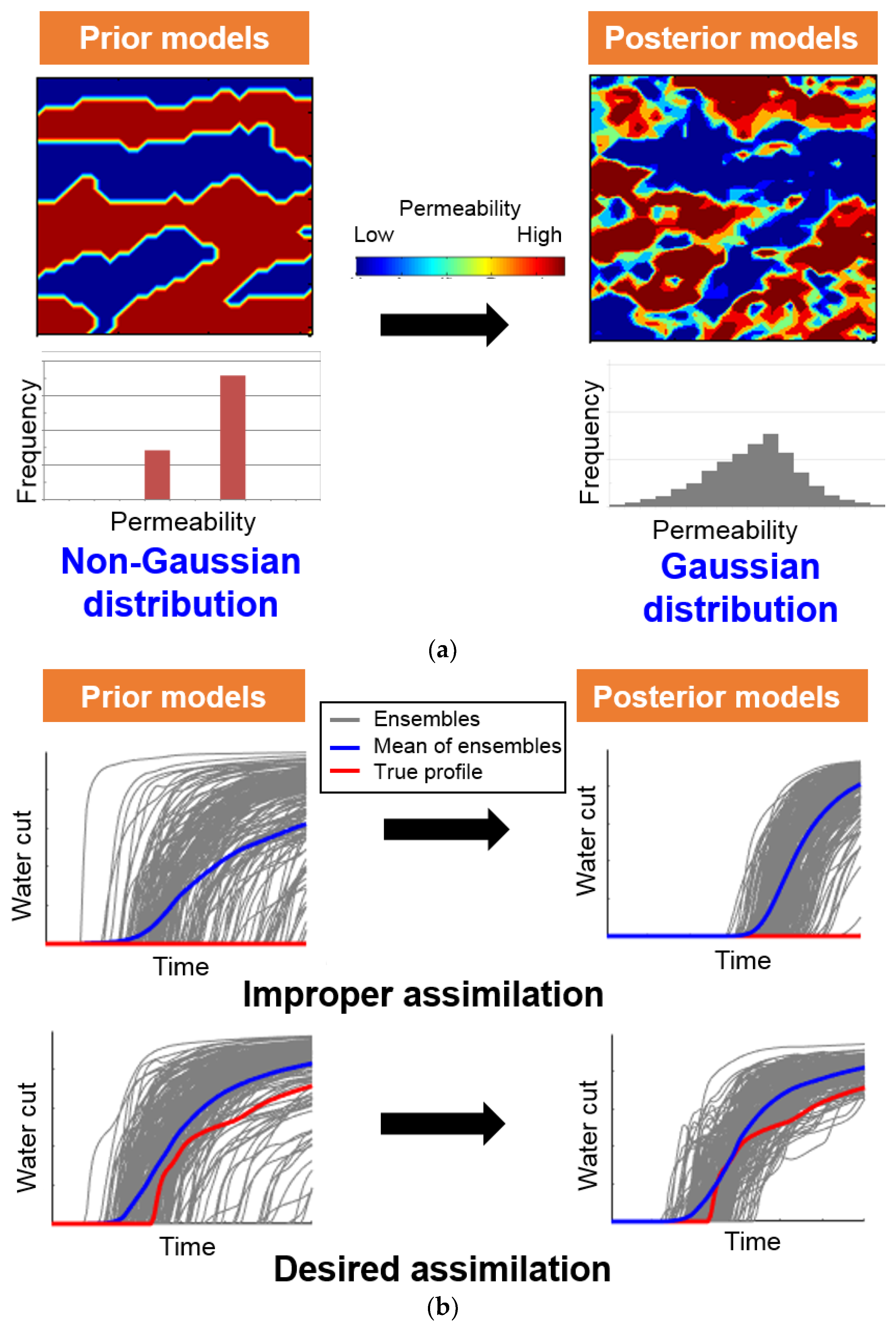
The statistical assimilation for high nonlinear problems in reservoir characterization is fundamentally based on mathematical modeling with linear algebra, and thereby its assumptions cause a few limitations as follows: non-Gaussian model parameters, improper prior ensembles, and finite ensemble size (the number of ensemble members). First, an assimilation equation assumes the model parameters follow a Gaussian distribution. One of the strengths of ensemble-based data assimilation is a wide range of applications, since there are few applicable constraints of model parameters in state vectors, e.g., permeability, facies, aquifer size, and relative permeability. However, most properties in reservoir engineering do not satisfy this Gaussian condition, e.g., some facies models in channelized reservoirs follow bimodal distributions. To make this matter worse, the updated model parameters tend to follow a normal distribution (see Figure 1a). This violates preservation of geological realism, and static information from well logging, core, and seismic data. The second weakness is the improper ensembles: the improper prior ensembles might induce unreliable estimation of posterior solutions. The mean value of initial ensembles is assumed to be true, in spite of inevitable error. A misfit between individual geomodel and true reservoir calculates an estimate error covariance, but a lot of actual fields are lacking in available data for making suitable prior datasets. To make this matter worse, the severe reservoir heterogeneity hinders the proper design of prior models. The uncertainty range of prior ensembles cannot even include observed data (see Figure 1b). Initial geomodels that are far off from the actual reservoir result in false convergence of updated models. The last is the problem of setting the proper size of ensemble. As regards the computation cost, the number of ensemble members must be small enough to be applicable in real fields, but it is difficult to confirm that the fixed ranges contain the true. When the ensemble size is too small, a cross-covariance can be mistakenly assessed [11,12]. Also, an ensemble collapse problem may occur due to small variance [13]. Therefore, the set of appropriate ensembles is essential. It is generally known that more than two hundred ensemble members are required for stable assimilation [14]. If geological uncertainty is too wide, or the inversion problem is very complex to assimilate recursively different-scaled dynamic data, more than four hundred ensemble members are needed [14].
For another research topic, the applicability of ensemble-based history matching has been expanded to various types of reservoirs. The principle of ensemble-based history matching is identical for all types of reservoirs. However, for each reservoir, detailed design and implementation of the method have evolved in different directions, reflecting their individual characteristics. It should be noted that different design and implementation of ensemble-based history matching, such as construction of a state vector, generation of initial ensembles, ensemble size, and supplementary techniques, are considered according to the reservoir type.
This paper introduces state-of-the-art ensemble-based methods with nonlinear problems, concentrates on EnKF and ES as frameworks in reservoir characterization, and also analyzes the aspect of overcoming weaknesses and developing schemes. The structure of this review is as follows: First, the mathematical frameworks of EnKF and ES are presented, together with their pros and cons. To mitigate the problems, recent progress is explained for strongly nonlinear problems. The case studies implementing ensemble-based data assimilation, categorized as reservoir characteristics like naturally fractured reservoir, channelized reservoir, and tight reservoir with hydraulic fracturing, are reviewed. In the conclusions, the recent progress of ensemble-based data assimilation is summarized, and future works are discussed.
2. Theoretical Framework of Ensemble–Based Data Assimilation
2.1. Mathematical Formulation
Ensemble-based methods consist of prediction and assimilation steps. After generating initial (or prior) values using the static data given, they are implemented by reservoir simulator to predict reservoir performances at observation time of dynamic data as Equation (1):
where, the function f represents a forward model, i.e., reservoir simulation. The input parameter, , stands for the i-th model parameters, which will be calibrated through ensemble-based methods, e.g., permeability, porosity, and facies. As initial condition, means dynamic conditions, such as pressure and saturation, for each grid, and d denotes dynamic data as the results of simulation, which will be compared with the observed data. Subscripts i and t mean indication of ensemble member and observed time step, respectively. Therefore, Ne indicates the number of total ensemble, and No represents the number of observation steps.
In this assimilation step, all equations are derived with the concept of state vector:
This state vector is updated by the product of the misfit between the observed data and the simulated data and the Kalman gain, K:
where, the superscripts a and p denote the assimilated and the prior state vector, respectively. H means the measurement matrix operator, which extracts simulation information from the state vector to compare with the observed data. The Kalman gain is constant for all ensembles, even though the observed data are also perturbed by the measurement error covariance, CD. Equation (4) for Kalman gain is derived by minimizing the posterior estimate error covariance, . For the purpose, the prior estimate error covariance, , is calculated by Equation (5). In the equation, the estimate error covariance is defined with the estimate error, e, which is the difference between the individual ensemble member and the true value. In ensemble–based methods, the mean of the state vector becomes the true vector, , due to their inherent assumption. Therefore, initial ensemble design is one of the key factors for successful application of ensemble-based history matching:
where, superscripts T and −1 mean the transpose and the inverse of the matrix, respectively.
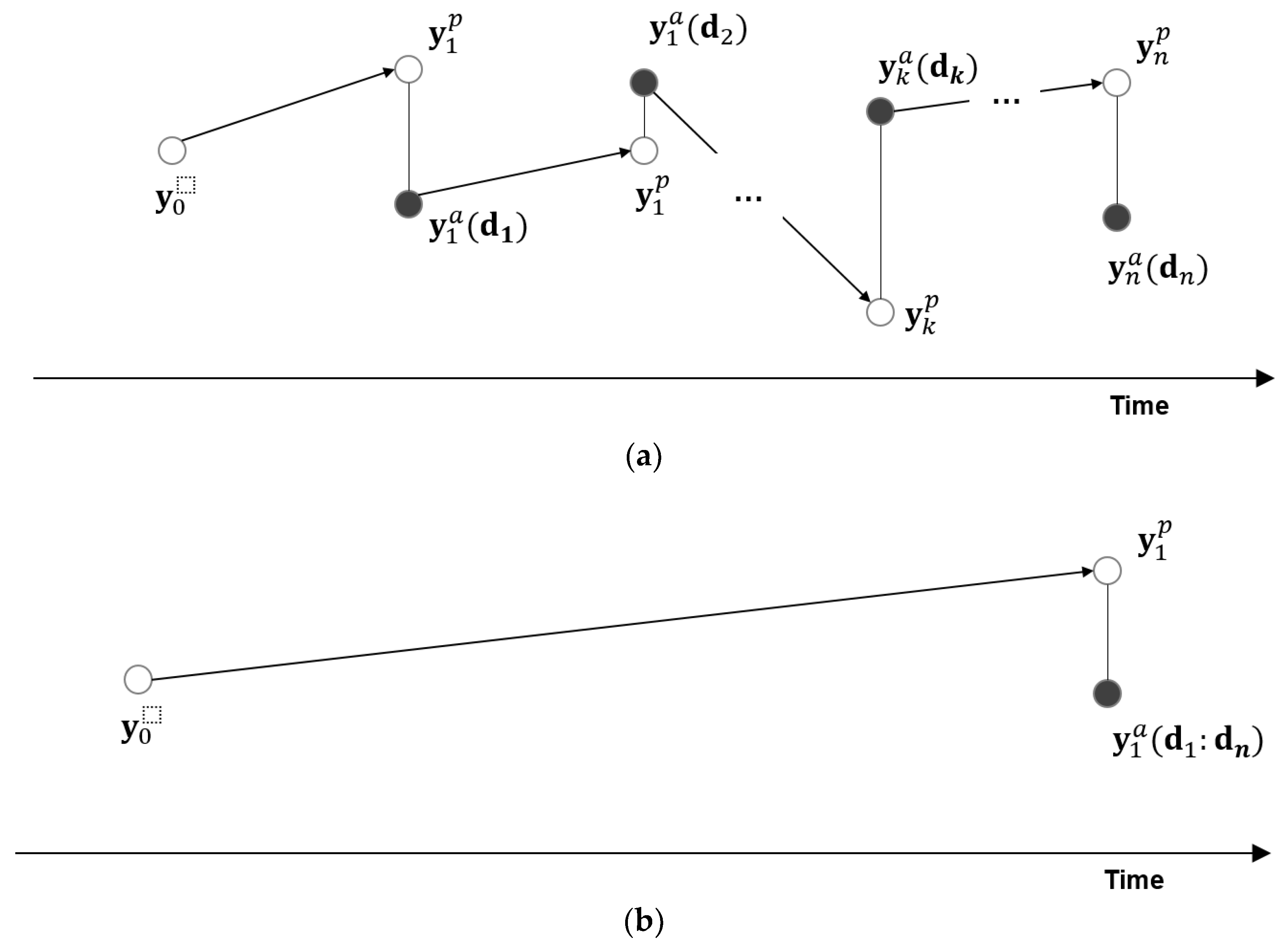
Basically, the above procedures are used for EnKF and ES in common, but they can be distinguished in terms of the number of updating the state vector and composition of the state vector. As described in Figure 2, prior models for EnKF are simulated and assimilated repeatedly until each measurement time, while prediction and assimilation for ES are conducted once until the last observation time, according to its global update strategy. In EnKF, after the updated state vector is obtained by Equations (3) and (4), they replace the prior state vector in the prediction step of Equation (1) to predict the reservoir performances at the next observation time. This two-step process is repeated until the last observation time step, No. ES, on the other hand, performs the prediction and assimilation process only once, with the observation data of all the time steps.
2.2. Characteristics of EnKF and ES
Conceptually, smoothing, filtering, and predicting can be explained in the time domain as below. These are determined depending on the relationship between the assimilation time, t and observation time, tn. If the assimilation time is larger than the observation time, it is a data smoothing problem; whereas, if assimilation is conducted at observation time, it is considered a filtering problem. The other case is a prediction problem, when the assimilation time is less than the observation time [4]:
- If tn < t: Smoothing (interpolation)
- If tn = t: Filtering
- If tn > t: Predicting
Both of the ensemble-based methods have strengths in common over other data assimilation methods, as below:
- Easy-coupling with forward models
- Various applications for model parameters
- Uncertainty analysis
- Well-established in mathematics
Table 1 summarizes the relative strengths and drawbacks of EnKF and ES. The only difference between EnKF and ES is whether the method is optimized considering the time dimension. EnKF repeats covariance minimization at each assimilation time, whereas ES includes the time dimension for optimization at a specific time. It is generally known that EnKF is superior to ES for nonlinear dynamic models. That is why EnKF has been widely used in the data assimilation of reservoir models, rather than ES [15].
In terms of simulation time, EnKF requires the number of Ne × No times of reservoir simulations, while ES needs Ne times of them. The difference in the number of reservoir simulations is very large, because normally the number of ensembles is around two hundred, and observations are available on a monthly basis. In the case of ES, the size of the state vector is larger than that of EnKF, due to the simulated data in Equation (1). However, this does not significantly affect the assimilation calculation, because the number of static and dynamic parameters in the state vector is much larger than the simulated data [16].
3. Methods to Overcome the Limitations of Ensemble–Based History Matching
Many researches have been conducted to solve the aforementioned limitations, e.g., non-Gaussian model parameters, improper prior ensembles, and finite ensemble size. The methodological efforts to improve the ensemble-based method are divided into three categories: (1) Kalman gain; (2) model parameters; and (3) observed dynamic data (see Figure 3). Figure 3 shows that the performance of ensemble-based method can be improved effectively through refinement of these key factors.
3.1. Importance of the Kalman Gain
Kalman gain is one of the most important factors in the ensemble-based method, because the assimilation equation is induced to minimize a posterior estimate error covariance. The Kalman gain is a weight of how much to reflect the difference between simulated and observed data to updated model parameters (see Equation (3)). Improvements of Kalman gain are covered as follows: localization, multiple Kalman gains, and regeneration of ensembles.
The goal of localization is to handle a spurious correlation between model parameters and observed data. In other words, localization is to identify the region that might be affected by observed data, rather than the whole reservoir. Model parameters near observation wells are properly correlated with the observed values, but parameters at distant locations are ambiguous to establish the relationship. Localization is a kind of weight function for an estimated error covariance. It alleviates the filter divergence problem, because it increases the degrees of freedom for observed data [17]. It is also one of the effective solutions when the ensemble size is small [11,18]. As the number of ensembles decreases, a cut-off radius decreases. The concept of localization can be divided into three categories, according to the following criteria:
- Distance (cut-off)
- Streamline or tracer simulation
Drainage area A covariance localization, as a solution to reduce ensemble size at the first suggested time, simply used a cut-off criterion based on the distance from the location of observed data to the location of a given state variable [11]. For example, the model parameters outside a certain area were excluded from data assimilation. Later, Schur product was applied to calculate a localized Kalman gain [18], which was an elementwise product between a correlation function and an estimate error covariance matrix. This concept gave more smoothed posterior parameters, than those from a cut-off localization. At gas reservoirs with aquifer, the exponential distance as a correlation function was investigated as the more suitable equation for localization [19].
Streamline-based covariance localization was implemented as an effective method to maintain geological realism, which used streamline trajectories to define the specific area influenced by a dynamic dataset [12,13,20]. It was able to reduce computation cost with small ensemble size (<100), by eliminating an area unrelated to the observed data [12]. The localization based on streamlines was more significant than a weight based on distance, because the streamlines were relevant to production data. Watanabe and Datta-Gupta expanded the concept of streamline localization according to fluid phase, and defined a correlation function from a phase streamline for each production data [13]. For example, water-cut (WCT) and gas-oil ratio (GOR) were coupled with water and gas streamlines, respectively. This flow-relevant localization could maintain geological realism, and gave a reliable uncertainty range without ensemble collapse. Jung and Choe distinguished the production-influenced area efficiently by comparing time-of-flight (TOF) from a phase velocity with the observation time of dynamic data [20]. As a limitation of steamline-based covariance localization, when a prior model covariance had a long correlation length, it would cause large local changes with loss of geological realism [17,21]. The requirement of different localization matrices came to the fore as a covariance comparison, i.e., covariance between the observed data and model parameters, and that between the observed data and primary variables [21]. In addition, the consideration of critical length was important at the high-order correlation function, e.g., fifth-order compact correlation function [22], and had to be determined including the degree of sensitivity of each observed data, and the correlation length of the geological model [17].
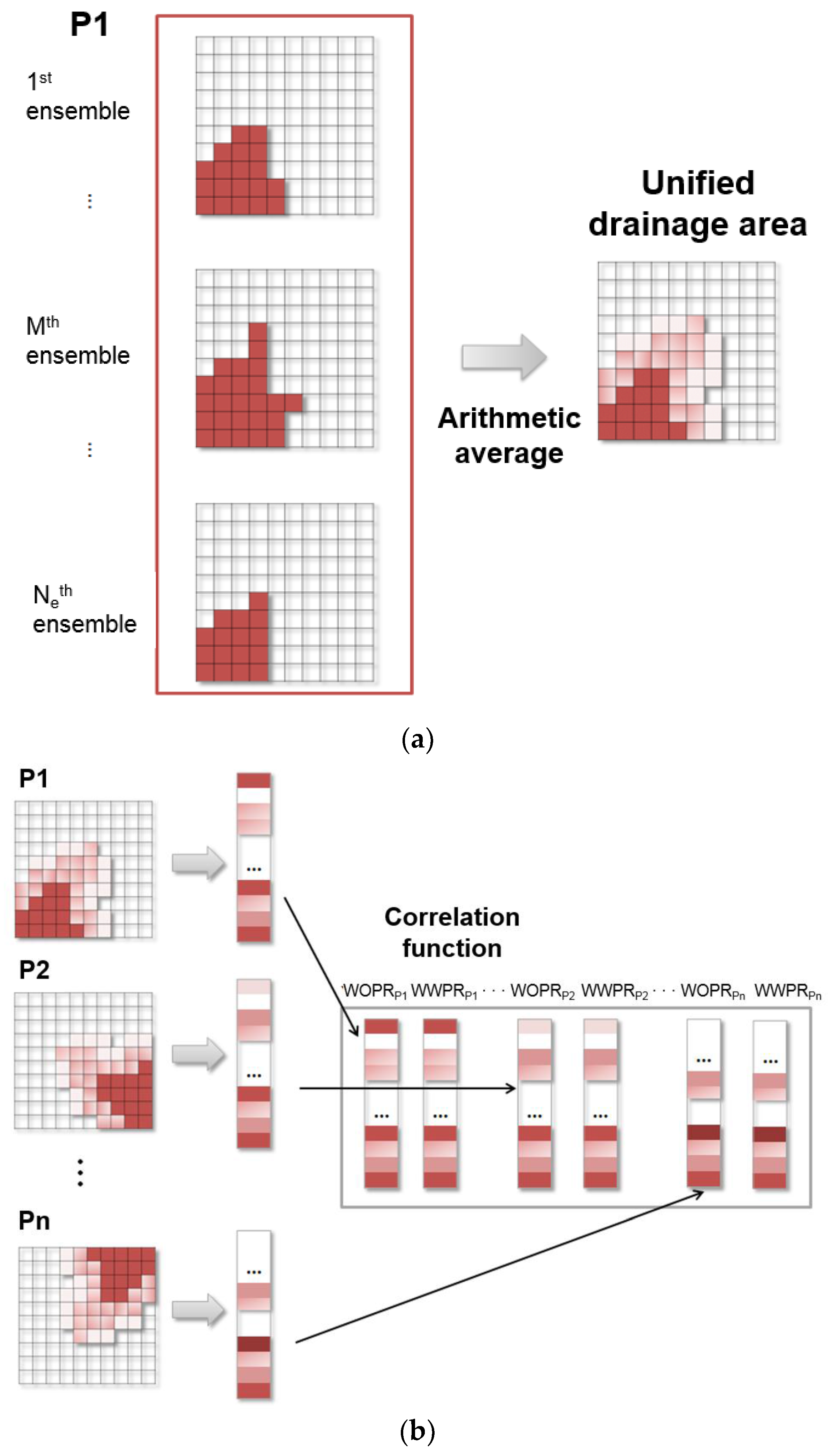
The covariance localization based on drainage area, determined by the pseudo-tracer of each well, was proposed [23,24,25]. The estimation of drainage area with drainage radius was shaped into a circle, but the reservoir heterogeneity could make for irregular shape [24]. Some schemes were studied to fix this matter, e.g., different localization concepts allocated at individual layers [24], and oil velocity field [25]. Figure 4 describes the concept of correlation function using hundreds of ensemble members [25]. Figure 4a shows a total Ne of 2D models with production well P1 in the lower left corner. When the drainage area is configured by a phase velocity from reservoir simulation, each model has a different drainage area, as shown in Figure 4. Although each model has a discrete drainage area, their mean has continuous values between 0 and 1. The vector of the unified drainage area for each production well in Figure 4b becomes a correlation function for localization. Here, the procedure for converting 2D models to column vectors, and for converting the vectors to the correlation matrix is exactly the same as the generation of a state vector and the estimated error covariance matrix in Equations (2) and (5).
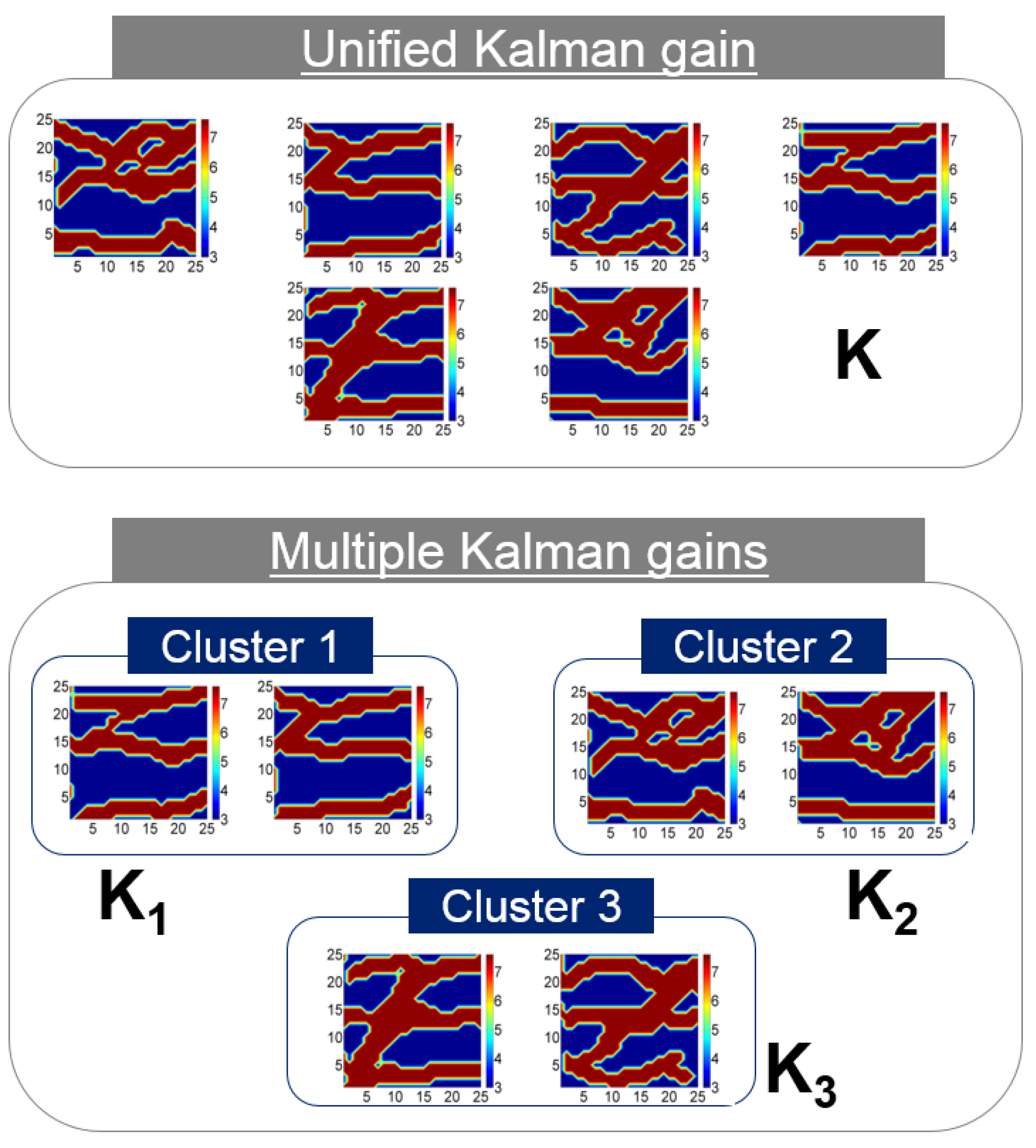
Another idea for Kalman gain is to utilize multiple Kalman gains, instead of a unified value [26,27,28,29,30]. It is reported that the role of Kalman gain is similar to that of a sensitivity matrix in the maximum posterior and randomized maximum likelihood [26,27]. However, the unified Kalman gain in the previous ensemble-based method is applied to the whole ensembles, although each ensemble member has a different sensitivity matrix. Multiple Kalman gains were introduced to EnKF [28] and ES [29,30], to apply more reliable Kalman gain for each ensemble member in Equation (3).
This concept assumes that reservoir models can be grouped by their similarity. To satisfy the assumption, distance-based clustering was utilized. After clustering, the reservoir models within the same cluster had more similar sensitivity matrices than those of other clusters (see Figure 5). Kalman gain is calculated for each cluster separately. This idea is especially useful for the channelized reservoir, because its heterogeneity is very high, and the difference in reservoir parameters between sand and shale facies is large. Also, channelized reservoirs can be transformed into a discrete model based on facies, so it is easy to apply image recognition algorithms. In previous research, the Hausdorff distance was successfully applied to 2D and 3D channel models. The larger the Hausdorff distance between the two models, the greater the difference between the two models. After calculating the distance, unsupervised learning algorithms, such as k-means or self-organizing map, can classify similar models based on the distance. However, this approach requires additional calculation for clustering, and the result of assimilation is sensitive for the clustering.
The last method for Kalman gain is to regenerate the ensembles whenever the covariance becomes smaller than a predetermined criterion [31,32]. In the process of data assimilation using EnKF progresses, an estimated error covariance becomes small, although the average of ensembles approaches the true field [31]. If this phenomenon gets worse, there will be a filter divergence problem where the ensembles become too similar. The estimated error in Equation (5) becomes very small, which results in small Kalman gain. Consequently, the state vector in Equation (3) cannot be calibrated, because the Kalman gain is small, even if the difference between the observed data and the simulated data is large. That is, there is no correction effect, even if there are additional observation data.
To solve this problem, a re-sampling method to mitigate filer divergence was developed, re-generating a set of ensembles, using both hard data and pseudo-hard data [32]. Here, hard data means given static well data, which data were used for building prior models by geostatistics. Pseudo-hard data can be generated from the updated ensemble member at the current time step. If the uncertainty of the value of the specific grid is small in the calibrated model, the value of the grid is used as input data to the geostatistics. Newly generated models replace updated models at the current time step, and the next prediction and assimilation are implemented with the new models. These procedures are repeated during recursive updates, whenever the covariance became smaller than a predetermined criterion.
3.2. Modification of Model Parameters
The typical assumptions of ensemble-based methods cause constraints on model parameters: Model parameters should follow Gaussian distribution, the mean of which is assumed as the true value of the given parameter, even though there is inevitable error. Previous researches have solved the concept of transformation and initial ensemble design. The most common conversion of model parameters is a log-normal distribution transformation. When permeability was a concerned model parameter in state vector, it was converted to a normal distribution by the transformation, because permeability is known to follow a log-normal distribution. Updated logarithmic permeability was transformed inversely to the original distribution on the prediction step (see Equation (1)). Recently, a lot of transformation or feature extraction techniques have been used for the conversion of model parameters, as follows:
- Normal score transform (NST)
- Discrete cosine transform (DCT)
- Level set function (LSF)
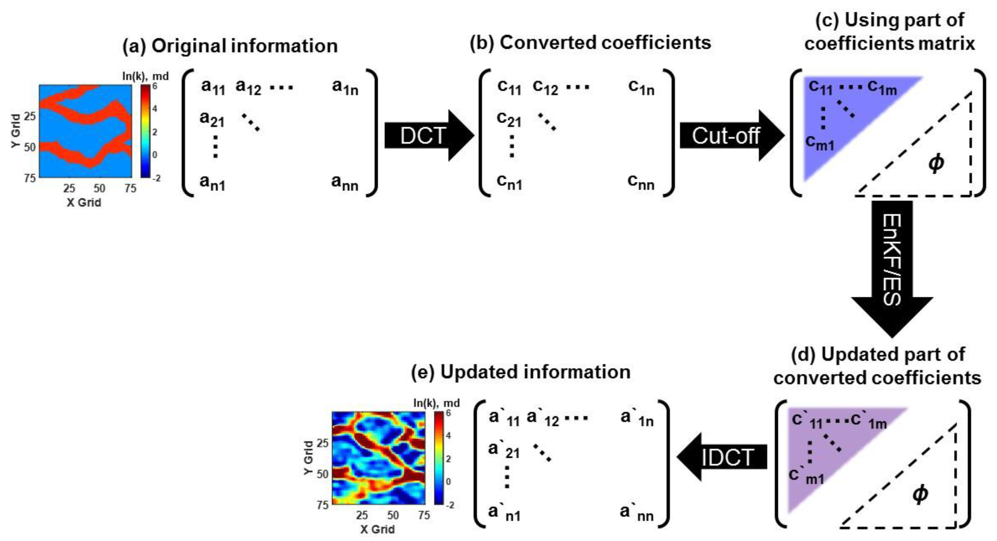
To assess the geological uncertainty, NST was used to convert non-parametric permeability to Gaussian distribution. The empirical cumulative distribution function (CDF) of model parameter was transformed into the corresponding quantile in CDF of standard normal distribution. This approach is useful, because any distribution could be converted to a standard normal distribution, which satisfies the Gaussian assumption in ensemble-based methods [33,34]. DCT is a method of representing audio or image information as a sum of cosine functions of different frequencies. The coefficient of the cosine function has overall information at a low frequency, and stores detailed information at a high frequency. It has been known to be an efficient tool to extract some significant features similar to principal component analysis (PCA), with respect to computational cost and prior information of error covariance [35,36,37,38]. Reservoir characterization with geological realism implemented DCT in channelized reservoir [34], and heavy oil reservoir [38]. Figure 6 describes the workflow of DCT by updating coefficients to update model parameters, instead of using the original model parameters [38]. LSF has been applied to separate a certain domain or shape into subdomains, which are set positive or negative signs with a zero-level set boundary. In reservoir characterization, it has been performed to parameterize facies models, as an effective scheme to convert a Gaussian distribution with facies preservation [39,40,41]. The concept of preservation of facies ratio was utilized for the transformation of updated parameters, not prior parameters [42]. After the updated parameter for each grid was arranged in descending order, facies were assigned to each grid based on the facies ratio. This method could not only preserve the facies ratio, but also mitigate the overshooting problem. These transformation methods could satisfy the Gaussian assumption in the assimilation step, but they had a problem in applying to discrete model parameters, such as facies, due to continuous values after assimilation. Also, the cut-off for determination of low frequency was not clear for transformation.
Many reports have underlined the importance of ensemble design to the ensemble-based method [14,15,43,44,45]. Some emphasized posterior ensembles obtained by combining prior ensembles [15,43]. When initial models are built by different geostatistical parameters, e.g., training image (TI) from the reference field, updated ensembles cannot provide reliable uncertainty ranges [14]. As an assimilation progresses, ensembles gradually converge to the mean of ensembles different from the reference model, which can require a sufficiently large number of ensembles to ensure reliable performance. The easiest way to include the true model in the range of initial models is to generate lots of ensembles that reflect geological uncertainties. Previous researches into uncertainty quantification built initial models through wide ranges of geostatistical parameters. In two-point simulation, correlation length and anisotropy parameters were utilized to design ensemble models [44,46]. In multiple-point simulation, lots of TIs were used to make hundreds of facies models [47,48]. However, the larger the geological uncertainty, the greater the ensemble size needed. This caused a burden of simulation cost. Researches on ensemble design are categorized as follows:
- Sampling
- Assimilation of uncertain geological factors
The use of a sampling scheme was to represent the characteristics of initial ensembles with low computational costs, reducing the reservoir simulations. The representative methods were singular value decomposition (SVD) [49], and distance-based clustering [50,51]. The selected models using these sampling methods were simulated with time-consuming reservoir simulators, instead of all models in the population set [51].
Geostatistical approaches, e.g., variogram and TI, have dealt with geological uncertainty, but the variables used in these methods are uncertain. An assimilation of variogram variables using EnKF failed to search the proper geomodels, due to the high nonlinearity between variogram variables and flow responses [44]. A lot of equiprobable models could make this matter worse, by increasing computing time. Some works calibrated the grid properties, e.g., grid permeability, facies ratio, or mean value of permeability allocated to each facies [33,34]. However, it was hard to directly modify parameters for geostatistics from dynamic data, due to high nonlinearity. Also, it was difficult to get a converged model, because during model generation, there were still lots of equiprobable models using updated geostatistical parameters.
3.3. Adjustment of Observed Dynamic Data
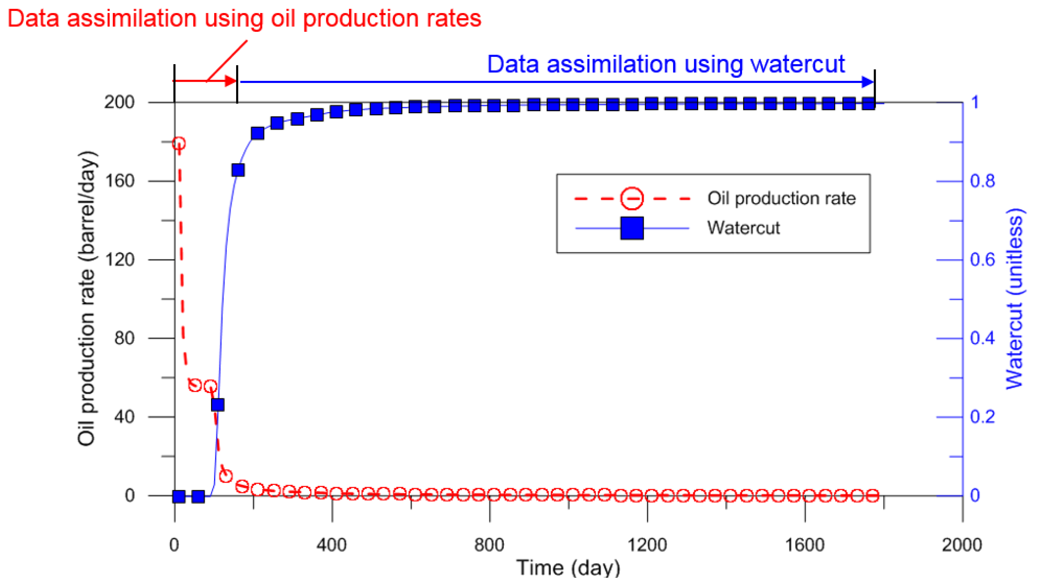
The last controllable parameter in an assimilation equation (refer to Equation (2)) is related to observed dynamic data. The topics of previous researches can be grouped as selective usage of observed data, and measurement error. It was recommended to use all available static data due to lack of data, while the dynamic data were preferable to utilize only essential observed data from sensitivity analysis [30,31]. A reliable data-analysis should exclude meaningless, erroneous, or inconsistent data. Figure 7 shows the unexpected effects of production performances in waterflooding at the channelized reservoir. The waterfront significantly changed the oil production and watercut before and after water breakthrough. This abrupt change of production performances regardless of spatial characteristics with static data could cause failure of data assimilation, and thereby result in unrealistic history matching. To solve this problem, some researchers used a few chosen performances, instead of all available dynamic data, e.g., exclusion of BHP during the shut-in period [30], or well flowing bottom hole pressure reaching the operational constraints [52].
One of the advantages of the ensemble-based method is that various observed data are used together efficiently. In other words, the observed data in Equation (3) consist of various measurement data, such as pressure, rate, and dimensionless-parameters, and they are not required pre-processing like normalization. Proper measurement error has to be set depending on the type of observed data, because the common range or magnitude of the observed data is different for each type.
4. Applications of Ensemble-Based History Matching in Reservoir Simulation
Early studies on assisted history matching using the ensemble based method were concentrated on synthetic fields, such as PUNQ-S3 [26,30,52,53,54,55], Brugge [56,57,58], or other synthetic fields customized for research objectives [59,60,61]. They tried to represent the advantages of EnKF and ES over gradient-based methods, such as genetic algorithm, simulated annealing, or other conventional methods. After the methods were verified in the history-matching problem, many researches have been targeted on resolving typical problems of ensemble-based history matching, as investigated in the previous section. At the same time, other efforts have been made to improve its applicability to various reservoir types.
Initial applications of ensemble-based history matching were limited to typical heterogeneous reservoirs, which have porous formation, with conventional completion and production mechanisms. However, many researches have been expanded to various types of reservoirs, such as naturally fractured reservoirs [60,62,63], channelized reservoirs [28,29,34,36,64,65], unconventional reservoirs [61,66,67], gas reservoirs [19,37,50], and others. Depending on the type of reservoir, the particular parameters, in addition to rock properties, can be included in the state vector. Facies ratio for channelized reservoir, fracture half-length for unconventional reservoir, and aquifer strength for gas reservoir are good examples of this. In addition, 4D seismic data, acoustic impedance, or Poisson’s ratio have been used for assimilation, as well as production data [68,69,70]. Recently, history-matching with production data has been successfully conducted in a large field with 60 million active gridblocks [71]. The full-field model was decomposed into six sector models by streamline maps, and each individual sector model was assimilated with local observations. Then, the assembled full-field model was assimilated again with observations from the full-field. This incurred tremendous computing costs, but computing time could be reduced significantly by decomposition and parallel computing scheme with ES.
Application examples of three reservoir types, naturally fractured reservoir, channelized reservoir, and tight reservoir with hydraulic fracturing, are presented. Reservoir parameterization and initial ensemble generation according to the reservoir type will be demonstrated in detail.
4.1. Naturally Fractured Reservoirs
Numerical simulation for the naturally fractured reservoir was usually conducted by the dual porosity-dual permeability model [72]. This can mimic production behaviors affected by the fracture network in the reservoir. It assumed that the matrix acts as hydrocarbon storage toward fracture, and fracture takes the role of conduits for fluid flow. Static data for the dual-porosity model consists of permeability and porosity for fracture, porosity for the matrix, and other parameters. The dual-porosity model has two additional parameters, interporosity flow coefficient and storativity ratio, which explain the phenomena in naturally fractured reservoirs. The interporosity flow coefficient can describe how quickly hydrocarbon fluid can flow from matrix to fracture through different porosities. As the coefficient is decreased, the transition from matrix to fracture is delayed. The other parameter, storativity ratio, represents the ratio of the reserves inside the fractures, to all the reserves. For history matching representing complex production behavior in naturally fractured reservoirs, more static data, as well as these additional parameters, are added into the state vector in Equation (1). The large number of unknown parameters increases the degree of freedom; thus, generation of the initial ensemble honoring static data is the most important factor for reliable history-matching reducing the uncertainty.
Table 2 compares the application examples of ensemble-based history matching for naturally fractured reservoirs. The component of a state vector can be different, depending on the generation method of the initial ensemble. When considering anisotropy using the discrete fracture network (DFN), the state vector includes the permeability tensor. Sigma factor, which is one of the parameters of dual porosity model for the fractured reservoir, can optionally be included in a state vector, as considered in [62]. Covariance localization [60], or refinement with velocity [63], can ensure numerically stable results, in spite of the small size of ensemble of around fifty.
An ensemble-based history matching was applied in naturally fractured tight reservoirs. The objective of the study was to prove the applicability of the proposed method to naturally fractured reservoirs. The authors created a simple synthetic reservoir, assuming that the orientation and location of the fractures were known approximately from seismic, microseismic, and core samples. The reservoir has a simple fracture network with several perpendicular fractures, and four production wells. Two of them share the fracture network connected to each other, one is completely in the isolated fracture, and the other is located in the matrix.
First of all, the dual porosity-dual permeability (DPDP) model was proposed as a simulation model for the naturally fractured reservoirs. This made a reservoir simulation simpler, compared to the discrete fracture network model using local raid refinement (LGR). Since the orientation and location of fractures were assumed known, the next parameters to affect production behavior were the matrix permeability, matrix-fracture transmissibility, and fracture permeability. Thus, the state vector for EnKF was composed of matrix permeability, fracture permeability, fracture porosity, and matrix-permeability transmissibility (sigma factor).
This study demonstrated that history matching with EnKF has the capability for fracture characterization and reserve estimation. When it estimated future production after history matching with only 20% of total production life, the production forecast showed good agreement with the true production behavior. Even though the application was simple, it validated the applicability of EnKF for history matching in naturally fractured reservoirs.
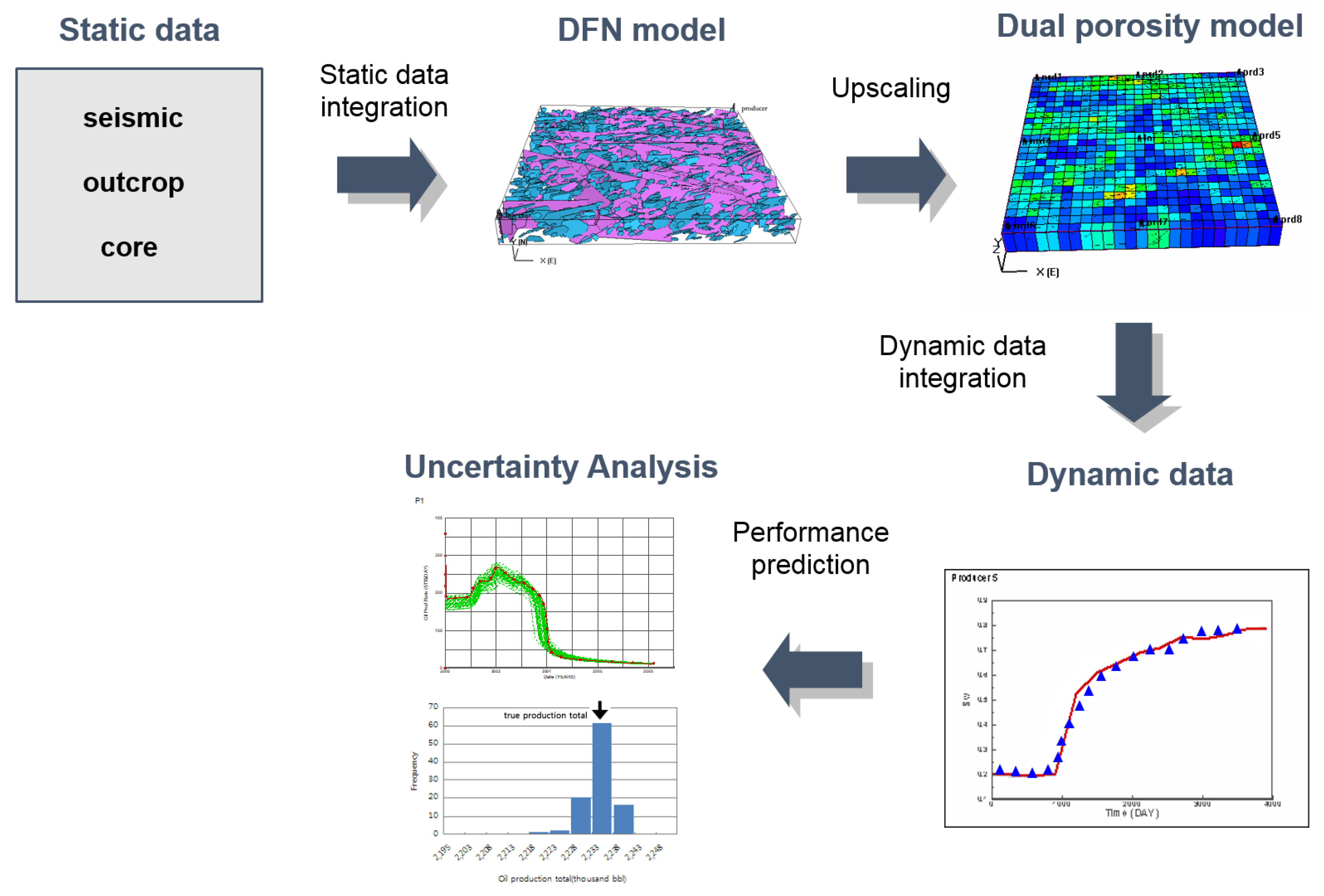
An application of EnKF to history matching considering the uncertainty of a naturally fractured reservoir [60] was published. Figure 8 shows its workflow that integrates fracture properties. Available static data that can be gathered in naturally fractured reservoirs include statistical data about the fracture network, such as fracture density, half-length, orientation, and aperture size. These data are just distributions in a certain region, and do not contain geographic reservoir properties of the whole region. That is why a geographic history-matching calibrating fracture distribution is needed.
In the research, an initial ensemble was constructed by DFN model from fracture statistical data, and converted into an equivalent model to the porous reservoir by the Oda method [73]. The converted model, which consists of permeability tensor, porosity for matrix and fracture, and interporosity flow coefficient, can be simulated, just like conventional reservoirs. These equi-probable reservoir models for initial ensemble honor statistical fracture data from the aspect of regional average properties, but heterogeneity within the region is not reflected at all. Thus, history-matching using dynamic data should be needed. Covariance localization was selected to overcome the typical limitations of EnKF. The concept is a selective assimilation that each type of observation identifies each influenced region by the time of flight (TOF) of the streamline simulation, and then assimilates reservoir properties within the influenced region through EnKF. The correlation function is calculated by averaging the influence region of ensemble members, as shown in Figure 4.
The method was applied to a producing inverted 9-spot reservoir with one injector and nine producers. The research verified the proposed scheme integrating DFN and EnKF for naturally fractured reservoirs. Covariance localization by streamline simulation can make EnKF more stable and reliable against overshooting or the filter divergence problem, notwithstanding the small ensemble size of 40. It could reproduce a reservoir model that is consistent with the true reservoir, and accurately estimate reserves of the field with an uncertainty assessment. As the results of production were forecast for 880 days after history-matching with production data for the initial 120 days, the coefficient of variant for reserves estimated of the history-matched ensemble member was reduced to 32%, compared to those of the initial ensemble member.
Another application for naturally fractured reservoirs is a study to estimate fracture effective permeability by upscaling using EnKF [63]. Its assumptions are quite different from the previously mentioned study. The authors assumed that the information of the fracture network is already known, and tried to characterize the permeability distribution of the matrix. The number of ensemble members was only 40, and each initial ensemble was generated by overlap of the assumed fracture network on the realization of matrix permeability using sequential Gaussian simulation (SGS). The integration was conducted by the local-global upscaling (LGU) method, which calculates coarse scale permeability using local boundary conditions determined from global coarse-scale flow solutions. History matching using production data was accomplished for the coarse-scale field by EnKF. Additionally, to overcome the limitation of the typical weakness of EnKF, the effective permeability distribution was refined with the velocity field after history matching.
This scheme was applied to a synthetic field, which is a 2-dimensional model of 1000 ft by 1000 ft. The reservoir produced oil with an inverted 5-spot system. Thus, the oil rate from four producers and bottomhole pressure from an injector were used for history matching as observation data. This study was designed to investigate the effects of LGU, EnKF, and refinement with velocity field (RVF). EnKF with LGU accomplished the history matching with low error between the estimated and actually observed dynamic parameters. However, the velocity and water saturation fields showed different shapes with smearing edges, compared to the reference field with fine-grid system. This weakness was improved by additional implementation of RVF. It was concluded that RVF can calibrate naturally fractured reservoir models more accurately, reflecting contrast characteristics of flow behavior between matrix and fracture.
4.2. Channelized Reservoir
A channelized reservoir consists of two kinds of deposits; one is high permeable sand with a longitudinally propagated narrow band, and the other is less permeable shale background. The permeability of this kind of reservoir is a bimodal distribution. The characteristics of the production behavior depend on the connectivity of the sand channel stream. Only when a producer is connected to a water injector, can it be expected that pressure support and oil are incremental with the results of water injection. Due to these geologically complex characteristics of the channelized reservoir, application of ensemble-based history-matching for these reservoirs has been a challenging topic. Many technical approaches linked with EnKF or ES have been adopted to resolve this problem; DCT, discrete wavelet transform (DWT), and other geostatistical methods reflecting the properties of channelized reservoirs.
Meanwhile, Table 3 summarizes other considerations for channelized reservoir that are already customized. The state vector in the majority of researches for channelized reservoir consisted of only permeability. This is because parametrization for the channelized reservoir is simple, and permeability is the best parameter to distinguish permeable sand from shale background. SNEsim (single normal equation simulation), which is one of the most representative algorithms in multiple point simulation, was commonly used for generating initial ensembles. Recently, new schemes of assisted history-matching, such as iterative adaptive Gaussian mixture filter (IAGM) [64], or ensemble smoother with clustered covariance (ESC) [65], have been conducted for efficient and reliable results.
Jafarpour and McLaughlin derived important implications for proper ensemble design, when EnKF was applied for history matching in channelized reservoirs [14]. The authors designed several experiments to quantify the effects of the ensemble generation method and number of ensemble members. Generally, initial ensembles for channelized reservoirs are generated by the multipoint geostatistical simulation method, and its accuracy is dependent on training images, which are used for the geostatistical method. When it is applied for EnKF, the training image to generate initial ensemble members should include uncertainties of width, tortuosity, connectedness, and complexity. If the initial ensemble did not include properties of the true field, the results of history matching were not reliable.
In the same context, the ensemble size should be designed to be large enough for each ensemble member to cover geological uncertainty. As the ensemble size increases, the initial ensembles can provide wider geological uncertainty. That is why ensemble size can affect the robustness and accuracy of EnKF. The study suggested that an ensemble size of 100 was too small for reliable results, while an ensemble size of 300 was sufficient for the case.
To complement a diversity of ensemble members, a probability weighted re-sampling coupled with EnKF was suggested [32]. The main idea of the study was to generate new ensemble members that reflect both the geological characteristics, and the early production data. The procedures were composed of generating the initial ensemble by SNESim, updating with EnKF, ensemble re-sampling with probability weighting, selecting re-sampling points and generating new ensemble members, and updating with EnKF for the next time step, repeatedly.
The method was implemented to a synthetic channelized reservoir with two distinct facies: sand and shale. An injector and a producer, drilled horizontally and completed with inflow control valves (ICV), were applied for a production scheme. History matching was conducted every month for the initial 9 months. Because ensemble variance diminished drastically after the 5th update, 20 ensemble members by re-sampling with the observed petrophysical properties were added. Re-sampling coupled with EnKF resulted in the reproduction of spatial continuity, and facies ratio consistent with the true field property.
One of the recent researches for channelized reservoirs is the ensemble smoother with clustered covariance as an assisted history-matching, proposed by Ref. [65]. The authors maintained that the proposed method could produce good performances for history-matching and production forecasts, by comparison with other methods, EnKF and ES. It differentiated assimilation procedures by clustering ensemble members. Clustered covariance can provide reliable Kalman gains, as shown in Equation (3).
The procedures of the method were initial facies modeling, clustering, and dynamic data assimilation using ES, as schematized in Figure 9. Initial facies models are generated with TIs and core data by SNESim, as mentioned before. The next process of the method is clustering. This consists of distance definition, dimension reduction, and clustering with K-means. Initial ensemble members are classified into several groups, and the criterion for classification is Hausdorff distance. The Hausdorff distance matrix was converted into an orthogonal coordinate system by multi-dimensional scaling. According to the converted distance in the orthogonal coordinate system, the ensemble members were clustered by K-means clustering. The main concept of the method was that each group of clustered models was assimilated by its own Kalman gain calculated from each group.
The research reported in [65] attempted to characterize the reference field on the assumption of the initial facies ratio. An initial ensemble of 200 members was generated, and then clustered into 10 groups. While the standard ES yielded an overshooting problem, the standard EnKF and the proposed ESC produced reliable results, representing the channel connectivity of the reference field without any numerical problem. However, the standard EnKF failed to conserve a bimodal distribution for permeability, and to accurately predict future production behavior. In spite of the initial assumption of lower facies ratio for sand over the reference field, the proposed ESC characterized the channelized reservoir with accurate facies ratio. Moreover, it represented production forecasts that were well-matched to the reference field, and efficient computation time, only 4.2% of the standard EnKF.
4.3. Tight Reservoir with Hydraulic Fracturing
In most of the tight reservoirs, hydraulic fracturing is a key factor for a commercially successful project. Optimization for a multi-stage fracturing process, such as design, implementation, and monitoring, is essential. Post-evaluation of hydraulic fracturing can be a most reliable basis to optimize the process of hydraulic fracturing. Despite its importance, there are not many researches on post-evaluation through history-matching in unconventional reservoirs. However, the environment of low oil price has yielded several researches on post-evaluation in multi-stage fractured reservoirs.
Table 4 summarizes three researches on ensemble–based history-matching for unconventional reservoirs. It was commonly assumed that reservoir properties are homogeneous, and that the fracture location for each stage is known. The reservoir model was calibrated by only the fracture half-length and permeability. A state vector can be constructed with the fracture half-length and permeability. In the case of Ref. [61], the fracture half-length can be defined by calibrated permeability, thus only the permeability was included in a state vector. However, observations were different, depending on the data gathering method. The methods of the three examples are different from each other: distributed temperature sensing (DTS), tracer test, and production logging tool (PLT). The observation parameter of each method corresponds to temperature, tracer concentration, and production rate, respectively.
Tracer test is widely conducted in the hydraulic fractured well, due to the convenience. It can diagnose the well performance in a very early stage of the production period, with relatively low cost. History matching with tracer test data for a hydraulic fractured reservoir was published in Ref. [67]. The reservoir model for this study assumed 4 stages of hydraulic fracturing.
A sensitivity study of fracture half-length and fracture permeability was performed, and the following conclusions made: the longer the fracture half-length, the larger the stimulated reservoir volume. Because the production data is dependent on SRV, the production data can be sensitive to the fracture half-length. Meanwhile, the fracture permeability did not affect the stimulated reservoir volume, but only the early production time of tracers. Thus, the tracer data is sensitive to fracture permeability.
The study quantified the effects of tracer and production data for ensemble-based history matching. The authors conducted three numerical experiments of history matching; with tracer data, production data, and both of them. History matching with tracer data characterized the fracture permeability accurately, but not the fracture half-length at all. In contrast, the production data characterized the fracture half-length accurately, but not the fracture permeability. The results of history matching with tracer and production data showed that the predicted fracture half-length and permeability showed good agreement with the true values. From the experiments, it was concluded that the tracer data during flowback and production data can be mutually complementary for characterization of hydraulic fractures by EnKF.
The applicability of EnKF was expanded to hydraulic fracture reservoir characterization using DTS [66]. DTS can be installed at wellbore, and provide temperature profile in real time during treatment, flow-back, and production period. In the case of DTS, temperature observation can be used in ensemble-based history-matching in unconventional reservoirs. In the research, temperature was observed at various locations of hydraulic fractures, and used as a history matching parameter. That is why they performed non-isothermal reservoir simulation by ECLIPSE 300 (Schlumberger, Houston, TX, USA). A sensitivity analysis was conducted to investigate the impact of DTS data with regard to reservoir and fracture parameters. The results of the analysis revealed that the impacts of the parameters in order are the number of fractures, reservoir permeability, fracture half-length, height, width, and fracture permeability, respectively. The purpose of the study was to estimate the hydraulic fracture geometry by integrating DTS observations. The authors selected two fracture parameters; one was the fracture permeability with small sensitivity, and the other was the fracture half-length with medium sensitivity. They organized an experiment to characterize the two parameters simultaneously with EnKF. Two parameters were assumed to be unknown, and the others constant.
The reservoir size and grid configuration of the example field were 3100 ft by 600 ft by 150 ft, and 100 by 40 by 30, respectively. The LGR was applied to neighboring grid blocks with hydraulic fractures for numerical stability. The total number of fracture stages was assumed to be eight, and the porosity and permeability of the reservoir were 30% and 0.2 md, respectively. The authors constructed an inverse model with fracture half-length and permeability as unknown parameters, and temperature as observation. The fracture half-length for the initial ensemble was generated randomly from a uniform distribution from (5 to 300) ft. The other unknown parameter, fracture permeability, was also generated randomly between (100 and 5000) md. The initial ensemble was calibrated by temperature profiles at seven time steps using EnKF. A wide range of uniform distributions with wide range at the initial stage turned into true values of fracture half-length and permeability as recursive updates. The study showed that the proposed scheme could make accurate estimates of fracture properties within only five updates during 100 days.
The last is an example using PLT data for ensemble-based history matching [61]. PLT has the advantage that it can gather production data of each fracture stage at bottomhole, not combined at the wellhead. However, PLT survey cannot be frequently conducted, due to the cost. A practical method was proposed to characterize each stage of hydraulic fractures, by integrating PLT data and production data with ES.
The key point of the study is how often PLT surveys are conducted. Frequent PLT data can improve the accuracy of history matching with ES. The author tried to seek a cost effective scheme to be applied in the industry. A controlled experiment was designed to quantify the effects of the number of PLTs on history matching with ES. In the study, there were three cases of data assimilation; with three times of production data, three times of PLT surveys, and one PLT survey and two production data. The results showed that only single PLT could significantly improve characterization of the fracture properties. Moreover, its estimate error was a similar level, compared to the case using two more PLT data.
5. Conclusions
This paper reviewed the historical development, as well as the recent progress, of ensemble-based history matching methods with data assimilation to solve nonlinear problems of static and dynamic data. The typical strengths of these methods are the easy integration of various data and mathematical clearness to reduce error covariance, while the weaknesses are the influences of the initial ensembles, e.g., non-Gaussian model parameters, improper prior ensembles, and finite ensemble size. To overcome these drawbacks, the studies have been to improve Kalman gains, the model parameters, and the observed dynamic data. Recent research trends can be categorized as two different directions: One trend is to improve the accuracy by mathematically resolving the inherent problems. The other trend is to enhance the field applicability by finding a proper combination of model parameterization, initial ensemble generation, and supplementary techniques, according to various reservoir types.
As regards representative challengeable works, new approaches to enhance the computation efficiency and to secure field applications are suggested. To improve accuracy, some methods have a tendency to sacrifice computational efficiency, by increasing the number of assimilation and ensemble member. As ES, compared with the computational efforts of EnKF, was developed to dramatically reduce the assimilation number, the paradigm shift to reduce simulation number can become a major research theme for ensemble-based techniques. A more reliable assisted-history matching tool, applicable to heterogeneous facies models, is required as well. To increase the applicability of heterogeneous reservoirs, the nonlinear relationships among static properties, dynamic variables, and observed scale-different data should be considered. Some unsolved problems should be included in current ensemble-based data assimilation, e.g., the preservation of geological realism, the reliable correlations between geological scenarios and reservoir properties, and uncertainty quantification with the results of many-objective history matching.
Acknowledgments
This study was supported by Basic Science Research Program through the National Research Foundation of Korea (NRF) funded by the Ministry of Education (2017R1D1A1B04033060) and by the Korea Institute of Energy Technology Evaluation and Planning (KETEP) and the Ministry of Trade, Industry and Energy (MOTIE), Korea (No. 20172510102150; No. 20172510102090), and also by Korea Institute of Geoscience and Mineral Resources (KIGAM) (GP2017-024).
Author Contributions
Seungpil Jung investigated various applications of ensemble-based history matching in reservoir simulation; Kyungbook Lee classified limitations of ensemble-based history matching and described representative methods to overcome each limitation; Changhyup Park identified the importance of ensemble-based data assimilation in the introduction and the conclusions; Jonggeun Choe participated in writing works and revised this manuscript.
Conflicts of Interest
The authors declare no conflict of interest.
References
- Blayo, E.; Bocquet, M.; Cosme, E.; Cugliandolo, L.F. Advanced Data Assimilation for Geosciences: Lecture Notes of the Les Houches School of Physics, 1st ed.; Oxford University Press: Oxford, UK, 2014; ISBN 978-0-19-872384-4. [Google Scholar]
- Evensen, G. Data Assimilation: The Ensemble Kalman Filter; Springer: New York, NY, USA, 2006; pp. 119–138. [Google Scholar]
- Asch, M.; Bocquet, M.; Nodet, M. Data Assimilation: Methods, Algorithms, and Applications, 1st ed.; Society for Industrial and Applied Mathematics: Philadelphia, PA, USA, 2016; ISBN 978-1-61-197454-6. [Google Scholar]
- Fletcher, S.J. Data Assimilation for the Geosciences: From Theory to Application; Elsevier: Amsterdam, The Netherlands, 2017; ISBN 978-0-12-804484-1. [Google Scholar]
- Griffith, A.K.; Nichols, N.K. Data Assimilation Using Optimal Control Theory; Numerical Analysis Report; The University of Reading: Reading, UK, 1994. [Google Scholar]
- Ide, K.; Courtier, P.; Ghil, M.; Lorenc, A. Unified notation for data assimilation: Operational, sequential and variational. J. Met. Soc. Japan 1997, 75, 181–189. [Google Scholar] [CrossRef]
- Zou, X.; Navon, I.M.; Ledimet, F.X. An optimal nudging data assimilation scheme using parameter estimation. Q. J. R. Meteorol. Soc. 1992, 118, 1163–1186. [Google Scholar] [CrossRef]
- Liu, C.; Xiao, Q.; Wang, B. An ensemble-based four-dimensional variational data assimilation scheme. Part I: Technical formulation and preliminary test. Mon. Weather Rev. 2008, 136, 3363–3373. [Google Scholar] [CrossRef]
- Bocquet, M.; Sakov, P. An iterative Kalman smoother. Q. J. R. Meteorol. Soc. 2013, 140, 1521–1535. [Google Scholar] [CrossRef]
- Oliver, D.S.; Reynolds, A.C.; Liu, N. Inverse Theory for Petroleum Reservoir Characterization and History Matching; Cambridge University Press: Cambridge, UK, 2008; pp. 347–366. [Google Scholar]
- Houtekamer, P.L.; Mitchell, H.L. Data assimilation using an ensemble Kalman filter technique. Mon. Weather Rev. 1998, 126, 796–811. [Google Scholar] [CrossRef]
- Arroyo-Negrete, E.; Devegowda, D.; Datta-Gupta, A.; Choe, J. Streamline-assisted ensemble Kalman filter for rapid and continuous reservoir model updating. SPE Reserv. Eval. Eng. 2008, 11, 1046–1060. [Google Scholar] [CrossRef]
- Watanabe, S.; Datta-Gupta, A. Use of phase streamlines for covariance localization in ensemble Kalman filter for three-phase history matching. SPE Reserv. Eval. Eng. 2012, 15, 273–289. [Google Scholar] [CrossRef]
- Jafarpour, B.; McLaughlin, D.B. Estimating channelized-reservoir permeabilities with the ensemble Kalman filter: The importance of ensemble design. SPE J. 2009, 14, 374–388. [Google Scholar] [CrossRef]
- Skjervheim, J.A.; Evensen, G. An ensemble smoother for assisted history matching. In Proceedings of the SPE Reservoir Simulation Symposium, The Woodlands, TX, USA, 21–23 February 2011. [Google Scholar] [CrossRef]
- Chen, Y.; Oliver, D.S. Ensemble randomized maximum likelihood method as an iterative ensemble smoother. Math. Geosci. 2012, 44, 1–26. [Google Scholar] [CrossRef]
- Emerick, A.; Reynolds, A.C. Combining sensitivities and prior information for covariance localization in the ensemble Kalman filter for petroleum reservoir applications. Comput. Geosci. 2011, 15, 251–269. [Google Scholar] [CrossRef]
- Houtekamer, P.L.; Mitchell, H.L. A sequential ensemble Kalman filter for atmospheric data assimilation. Mon. Weather Rev. 2001, 129, 123–137. [Google Scholar] [CrossRef]
- Kim, S.; Lee, C.; Lee, K.; Choe, J. Aquifer characterization of gas reservoirs using ensemble Kalman filter and covariance localization. J. Pet. Sci. Eng. 2016, 146, 446–456. [Google Scholar] [CrossRef]
- Jung, S.; Choe, J. Reservoir characterization using a streamline-assisted ensemble Kalman filter with covariance localization. Energy Explor. Exploit. 2012, 30, 645–660. [Google Scholar] [CrossRef]
- Chen, Y.; Oliver, D.S. Cross-covariances and localization for EnKF in multiphase flow data assimilation. Comput. Geosci. 2010, 14, 579–601. [Google Scholar] [CrossRef]
- Gaspari, G.; Cohn, S.E. Construction of correlation functions in two and three dimensions. Q. J. R. Meteorol. Soc. 1999, 125, 723–757. [Google Scholar] [CrossRef]
- Damiani, M.C. Determinacao de Padroes de Fluxo em Simulacoes de Reservatorio de Petroleo Utilizando Tracadores (In Portuguese). Master’s Thesis, Universidade Federal do Rio de Janeiro, Rio de Janeiro, Brazil, May 2007. [Google Scholar] [CrossRef]
- Emerick, A.A.; Reynolds, A.C. History matching a field case using the ensemble Kalman filter with covariance localization. SPE Reserv. Eval. Eng. 2011, 14, 443–452. [Google Scholar] [CrossRef]
- Yeo, M.J.; Jung, S.P.; Choe, J. Covariance matrix localization using drainage area in an ensemble Kalman filter. Energy Sources Part A Recovery Util. Environ. Eff. 2014, 36, 2154–2165. [Google Scholar] [CrossRef]
- Gu, Y.; Oliver, D.S. The ensemble Kalman filter for continuous updating of reservoir simulation models. ASME J. Energy Resour. Technol. 2005, 128, 79–87. [Google Scholar] [CrossRef]
- Zafari, M.; Reynolds, A.C. Assessing the uncertainty in reservoir description and performance predictions with the ensemble Kalman filter. SPE J. 2007, 12, 382–391. [Google Scholar] [CrossRef]
- Lee, K.; Jeong, H.; Jung, S.; Choe, J. Characterization of channelized reservoir using ensemble Kalman filter with clustered covariance. Energy Explor. Exploit. 2013, 31, 17–29. [Google Scholar] [CrossRef]
- Lee, K.; Jeong, H.; Jung, S.; Choe, J. Improvement of ensemble smoother with clustering covariance for channelized reservoirs. Energy Explor. Exploit. 2013, 31, 713–726. [Google Scholar] [CrossRef]
- Lee, K.; Jung, S.; Lee, T.; Choe, J. Use of clustered covariance and selective measurement data in ensemble smoother for three-dimensional reservoir characterization. J. Energy Resour. Technol. Trans. ASME 2017, 139, 022905. [Google Scholar] [CrossRef]
- Park, K.; Choe, J. Use of ensemble Kalman filter to 3-dimensional reservoir characterization during waterflooding. In Proceedings of the SPE Europe/EAGE Annual Conference and Exhibition, Vienna, Austria, 12–15 June 2006. [Google Scholar] [CrossRef]
- Nejadi, S.; Leung, J.; Trevedi, J. Characterization of non-Gaussian geologic facies distribution using ensemble Kalman filter with probability weighted re-sampling. Math. Geosci. 2015, 47, 193–225. [Google Scholar] [CrossRef]
- Jo, H.; Jung, H.; Ahn, J.; Lee, K.; Choe, J. History matching of channel reservoirs using ensemble Kalman filter with continuous update of channel information. Energy Explor. Exploit. 2017, 35, 3–23. [Google Scholar] [CrossRef]
- Jung, H.; Jo, H.; Kim, S.; Lee, K.; Choe, J. Recursive update of channel information for reliable history matching of channel reservoirs using EnKF with DCT. J. Pet. Sci. Eng. 2017, 154, 19–37. [Google Scholar] [CrossRef]
- Jafarpour, B.; McLaughlin, D.B. History matching with an ensemble Kalman filter and discrete cosine parameterization. Comput. Geosci. 2008, 12, 227–244. [Google Scholar] [CrossRef]
- Jafarpour, B.; McLaughlin, D.B. Reservoir characterization with the discrete cosine transform. SPE J. 2009, 14, 182–201. [Google Scholar] [CrossRef]
- Kim, S.; Lee, C.; Lee, K.; Choe, J. Characterization of channelized gas reservoirs using ensemble Kalman filter with application of discrete cosine transformation. Energy Explor. Exploit. 2016, 34, 319–336. [Google Scholar] [CrossRef]
- Panwar, W.; Trivedi, J.J.; Nejadi, S. Importance of distributed temperature sensor data for steam assisted gravity drainage reservoir characterization and history matching within ensemble Kalman filter framework. ASME J. Energy Resour. Technol. 2015, 137, 042902. [Google Scholar] [CrossRef]
- Moreno, D.L.; Aanonsen, S.I. Continuous facies updating using the ensemble Kalman filter and the level set method. Math. Geosci. 2011, 43, 951–970. [Google Scholar] [CrossRef]
- Lorentzen, R.J.; Flornes, K.M.; Nævdal, G. History matching channelized reservoirs using the ensemble Kalman filter. SPE J. 2012, 17, 137–151. [Google Scholar] [CrossRef]
- Lorentzen, R.J.; Nævdal, G.; Shafieirad, A. Estimating facies fields by use of the ensemble Kalman Filter and distance functions—Applied to shallow-marine environments. SPE J. 2012, 3, 146–158. [Google Scholar] [CrossRef]
- Kim, S.; Lee, C.; Lee, K.; Choe, J. Characterization of channel oil reservoirs with an aquifer using EnKF, DCT, and PFR. Energy Explor. Exploit. 2016, 34, 828–843. [Google Scholar] [CrossRef]
- Aanonsen, S.I.; Nævdal, G.; Oliver, D.S.; Reynolds, A.C.; Vallès, B. The ensemble Kalman filter in reservoir engineering—A review. SPE J. 2009, 14, 393–412. [Google Scholar] [CrossRef]
- Jafarpour, B.; Tarrahi, M. Assessing the performance of the ensemble Kalman filter for subsurface flow data integration under variogram uncertainty. Water Resour. Res. 2011, 47. [Google Scholar] [CrossRef]
- Oliver, D.S.; Chen, Y. Recent progress on reservoir history matching: A review. Comput. Geosci. 2011, 15, 185–221. [Google Scholar] [CrossRef]
- Lee, K.; Jo, G.; Choe, J. Improvement of ensemble Kalman filter for improper initial ensembles. Geosyst. Eng. 2011, 14, 79–84. [Google Scholar] [CrossRef]
- Scheidt, C.; Caers, J. Representing spatial uncertainty using distances and kernels. Math. Geosci. 2009, 41, 397–419. [Google Scholar] [CrossRef]
- Suzuki, S.; Caers, J. A distance-based prior model parameterization for constraining solutions of spatial inverse problems. Math. Geosci. 2008, 40, 445–469. [Google Scholar] [CrossRef]
- Kang, B.; Lee, K.; Choe, J. Improvement of ensemble smoother with SVD-assisted sampling scheme. J. Pet. Sci. Eng. 2016, 141, 114–124. [Google Scholar] [CrossRef]
- Kim, S.; Lee, C.; Lee, K.; Choe, J. Initial ensemble design scheme for effective characterization of 3D channel gas reservoirs with an aquifer. J. Energy Resour. Technol. Trans. ASME 2017, 139, 022911. [Google Scholar] [CrossRef]
- Kang, B.; Yang, H.; Lee, K.; Choe, J. Ensemble Kalman filter with PCA-assisted sampling for channelized reservoir characterization. J. Energy Resour. Technol. Trans. ASME 2017, 139, 032907. [Google Scholar] [CrossRef]
- Gao, G.; Zafari, M.; Reynolds, A.C. Quantifying uncertainty for the PUNQ-S3 problem in a Bayesian setting with RML and EnKF. SPE J. 2006, 11, 506–515. [Google Scholar] [CrossRef]
- Li, H.; Yang, D. Estimation of multiple petrophysical parameters for the PUNQ-S3 model using ensemble-based history matching. In Proceedings of the SPE EUROPEC/EAGE Annual Conference and Exhibition, Vienna, Austria, 23–26 May 2011. [Google Scholar] [CrossRef]
- Le, D.H.; Emerick, A.A.; Reynolds, A.C. An adaptive ensemble smoother with multiple data assimilation for assisted history matching. In Proceedings of the SPE Reservoir Simulation Symposium, Houston, TX, USA, 23–25 February 2015. [Google Scholar] [CrossRef]
- Nævdal, G.; Mannseth, T.; Vefring, E.H. Near-well reservoir monitoring through ensemble Kalman filter. In Proceedings of the SPE/DOE Improved Oil Recovery Symposium, Tulsa, OK, USA, 13–17 April 2002. [Google Scholar] [CrossRef]
- Emerick, A.A.; Reynolds, A.C. Ensemble smoother with multiple data assimilation. Comput. Geosci. 2013, 55, 3–15. [Google Scholar] [CrossRef]
- Peters, E.; Chen, Y.; Leeuwenburgh, O. Extended Brugge benchmark case for history matching and water flooding optimization. Comput. Geosci. 2013, 50, 16–24. [Google Scholar] [CrossRef]
- Chen, Y.; Oliver, D.S. Ensemble-based closed-loop optimization applied to Brugge field. SPE Reserv. Eval. Eng. 2010, 13, 56–71. [Google Scholar] [CrossRef]
- Wen, X.H.; Chen, W.H. Real-time reservoir model updating using ensemble Kalman filter. In Proceedings of the SPE Reservoir Simulation Symposium, Houston, TX, USA, 31 January–2 February 2005. [Google Scholar] [CrossRef]
- Jung, S. Stochastic Characterization for Fractured Reservoirs with Ensemble Kalman Filter. Ph.D. Dissertation, Seoul National University, Seoul, Korea, 2008. [Google Scholar]
- Jung, S. Integration of the production logging tool and production data for post-fracturing evaluation by the ensemble smoother. Energies 2017, 19, 859. [Google Scholar] [CrossRef]
- Ghods, P.; Zhang, D. Ensemble based characterization and history matching of naturally fractured tight/shale gas reservoirs. In Proceedings of the SPE Western Regional Meeting, Anaheim, CA, USA, 27–29 May 2010. [Google Scholar] [CrossRef]
- Tanaka, M.; Tanaka, S.; Arihara, N.; Okabe, H. Estimation of fracture effective permeability by upscaling using ensemble Kalman filter. In Proceedings of the Asia Pacific Oil and Gas Conference and Exhibition, Brisbane, Australia, 18–20 October 2010. [Google Scholar] [CrossRef]
- Sebacher, B.; Stordal, A.S.; Hanea, R. Bridging multipoint statistics and truncated Gaussian fields for improved estimation of channelized reservoirs with ensemble methods. Comput. Geosci. 2015, 19, 341–369. [Google Scholar] [CrossRef]
- Lee, K.; Jung, S.; Choe, J. Ensemble smoother with clustered covariance for 3D channelized reservoirs with geological uncertainty. J. Pet. Sci. Eng. 2016, 145, 423–435. [Google Scholar] [CrossRef]
- Tarrahi, M.; Gildin, E.; Moreno, J.; Gonzales, S. Dynamic integration of DTS data for hydraulically fractured reservoir characterization with the ensemble Kalman filter. In Proceedings of the SPE Biennial Energy Resources Conference, Port of Spain, Trinidad, 9–11 June 2014. [Google Scholar] [CrossRef]
- Elahi, S.H.; Jafarpour, B. Characterization of fracture length and conductivity from tracer test and production data with ensemble Kalman filter. In Proceedings of the Unconventional Resources Technology Conference, San Antonio, TX, USA, 20–22 July 2015. [Google Scholar] [CrossRef]
- Reiso, E.; Haver, M.C.; Aga, M. Integrated workflow for quantitative use of time-lapse seismic data in history matching: A North sea field case. In Proceedings of the SPE Europe/EAGE Annual Conference, Madrid, Spain, 13–16 June 2005. [Google Scholar] [CrossRef]
- Skjervheim, J.A.; Evensen, G.; Aanonsen, S.I.; Ruud, B.O.; Jonasen, T.A. Incorporating 4D seismic data in reservoir simulation models using ensemble Kalman filter. SPE J. 2007, 12, 282–292. [Google Scholar] [CrossRef]
- Emerick, A.A. Analysis of the performance of ensemble-based assimilation of production and seismic data. J. Pet. Sci. Eng. 2016, 139, 219–239. [Google Scholar] [CrossRef]
- Lin, B.; Crumpton, P.I.; Dogru, A.H. Field scale assisted history matching using a systematic, massively parallel ensemble Kalman smoother procedure. In Proceedings of the SPE Reservoir Simulation Conference, Montgomery, TX, USA, 20–22 February 2017. [Google Scholar] [CrossRef]
- Warren, J.E.; Root, P.J. The behavior of naturally fractured reservoirs. SPE J. 1963, 3, 245–255. [Google Scholar] [CrossRef]
- Oda, M. Permeability tensor for discontinuous rock masses. Geotechnique 1985, 35, 483–495. [Google Scholar] [CrossRef]
Figure 1.
Examples of unreliable results after assimilating the dynamic data through ensemble-based data assimilation: (a) The reservoir properties of the true case follow a non-Gaussian distribution (bimodal distribution), but the assimilated result shows a Gaussian distribution; (b) When prior models (grey lines) contain the true performance (red line), ensemble-based methods estimate the reliable assimilation for their mean values to converge the true profile.

Figure 2.
Comparison of sequence between (a) EnKF, and (b) ES: y and d mean a state vector and an observation vector, respectively. Superscripts p and a denote ‘prediction’ and ‘assimilation’, which processes are represented by arrow and solid line. The subscript number is the time step for the process. d1:dn means an observation vector, which consists of observations from the 1st to the n-th time steps. An open circle means a prediction step, while a dark circle is an assimilation stage.

Figure 3.
Classification of the methodologies to improve ensemble-based methods.
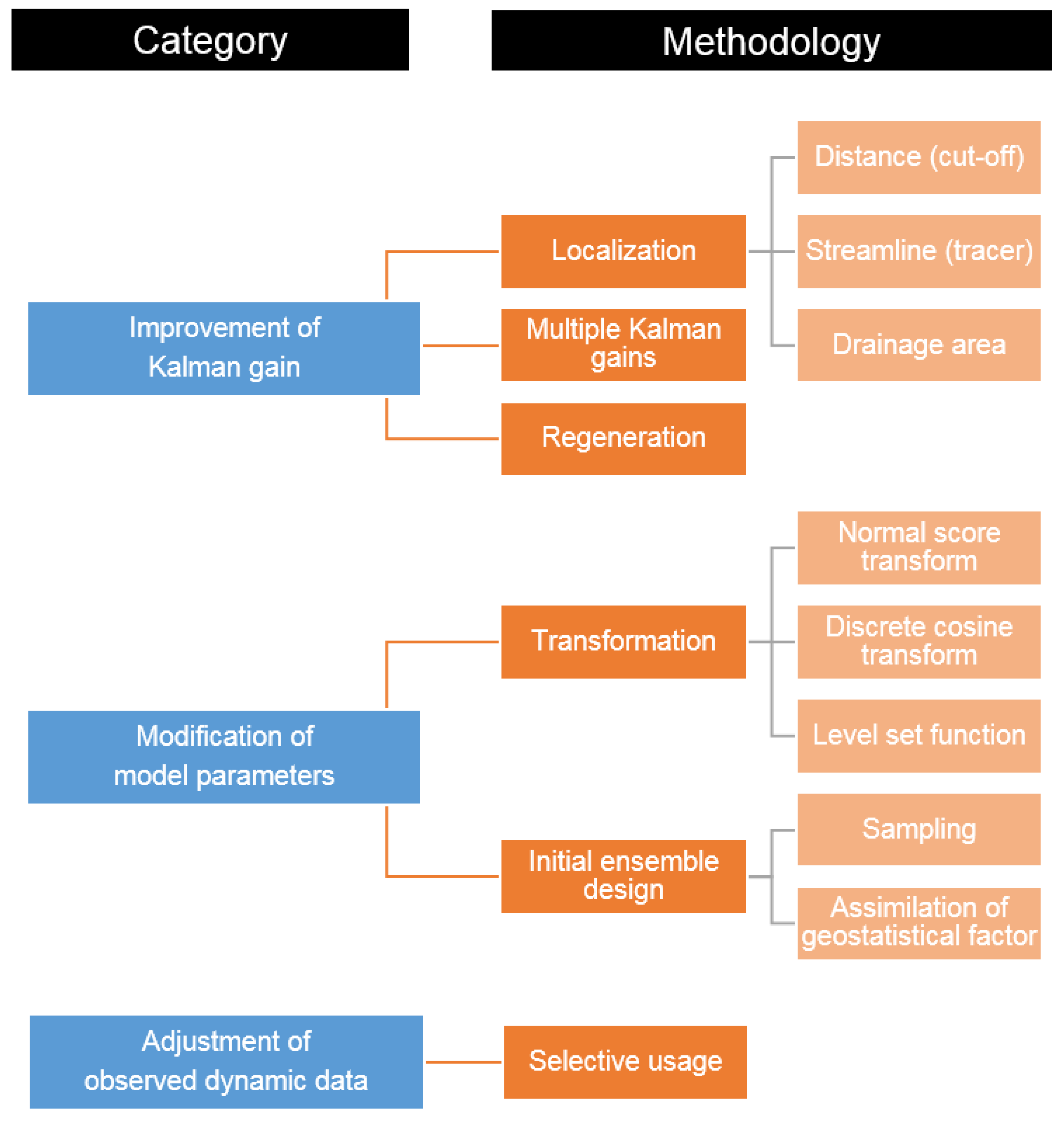
Figure 4.
The concept of correlation function for drainage area: (a) Definition of drainage area for each production well; (b) Construction of correlation function. WOPR is well oil production rate, and WWPR stands for well water production rate. P represents ‘the production well’, and the subscripts 1, 2, and n mean the indication number for each production well.

Figure 5.
The concept of multiple Kalman gains. The geological scenarios could be separated by clustering.
Figure 5.
The concept of multiple Kalman gains. The geological scenarios could be separated by clustering.

Figure 6.
The workflow of ensemble-based method with DCT. (a) An ensemble member can be transformed to a matrix (original information); (b) The original information is converted to coefficients through DCT; (c) Only the low frequency area (upper left triangle) is used for assimilation by the ensemble-based method; (d) The coefficients in the low frequency area are updated; (e) The updated coefficients are inversely converted to the updated information. IDCT stands for inverse discrete cosine transform.

Figure 7.
Example of selective usage of different observed data: As water breakthrough occurs, distinct separation of oil production rates from watercut is observed. Before the breakthrough, the oil production rates are the target of data assimilation; but after the water volume produced is significantly increased, the data assimilation should use watercut data, to obtain the reliability of ensemble-based methods.

Figure 8.
Workflow of fractured reservoir characterization and performance prediction.

Figure 9.
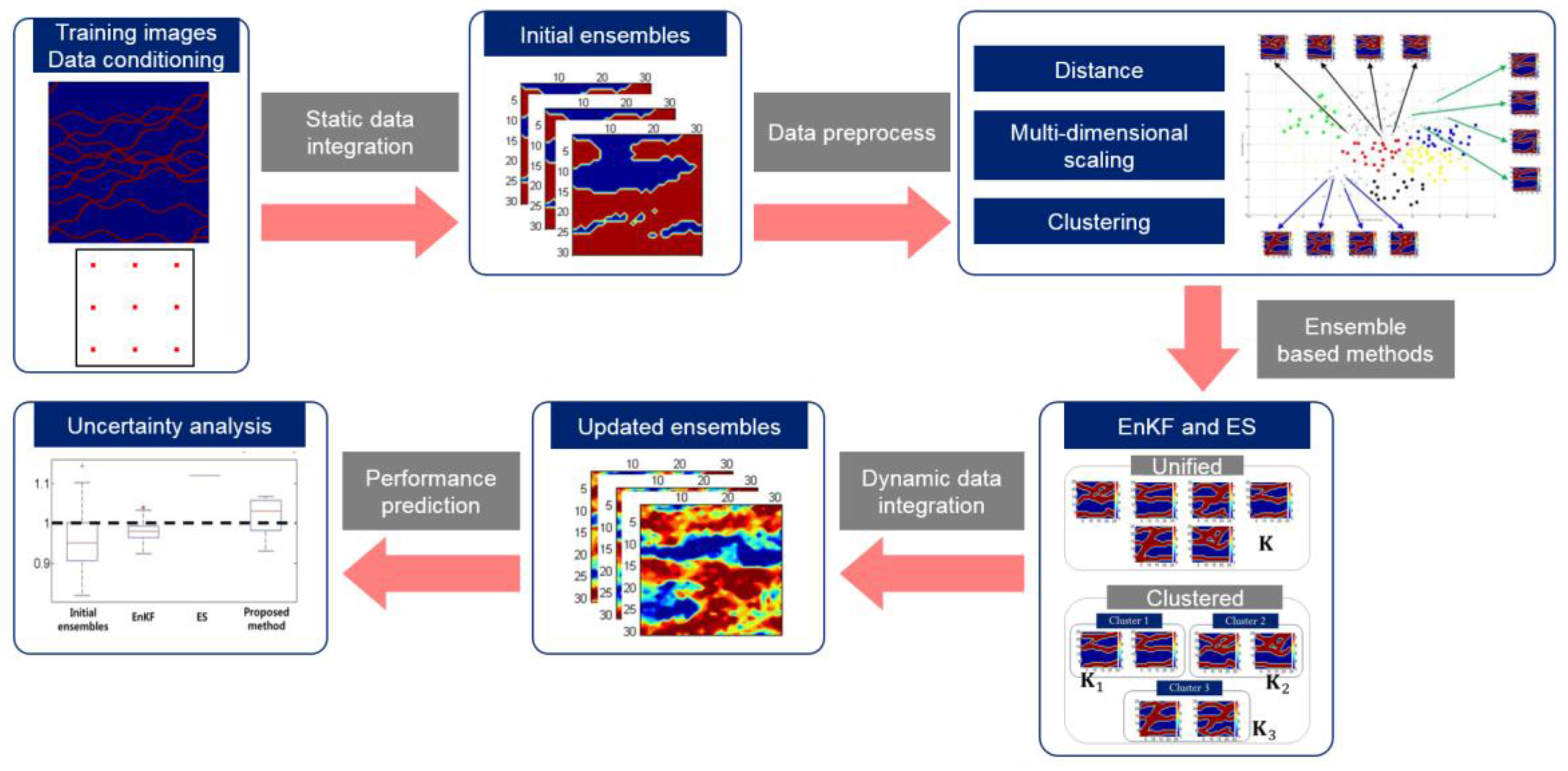
Typical workflow to forecast production performances integrating data clustering with ensemble-based methods at channelized reservoirs [65].
Figure 9.
Typical workflow to forecast production performances integrating data clustering with ensemble-based methods at channelized reservoirs [65].


Table 1.
Comparison between EnKF and ES.
| EnKF | ES | |
|---|---|---|
| Strength |
|
|
| Drawback |
|
|
Table 2.
Applications of ensemble based history matching for naturally fractured reservoirs.
| Jung [60] | Ghods and Zhang [62] | Tanaka et al. [63] | |
|---|---|---|---|
| No. of ensemble | 40 | 60 | 40 |
| state vectors | |||
| ∙ Model static | x-permeability y-permeability Fracture porosity | Fracture permeability Fracture porosity Matrix porosity Sigma factor | x-permeability y-permeability |
| ∙ Model dynamic | Water saturation Reservoir pressure | - | Water saturation Reservoir pressure |
| ∙ Observation | Bottom hole pressure Oil rate Water-cut | Gas rate Water rate | Bottom hole pressure Oil rate |
| Number of producer | 8 | 4 | 4 |
| Number of injector | 1 | - | 1 |
| Forward simulator | ECLIPSE 100 | ECLIPSE 100 | Streamline-based |
| Ensemble generation | DFN | Random | SGS and DFN |
| Assimilation method | EnKF | EnKF | EnKF |
| Supplemental Technique | Localization | - | Refinement with velocity |
Table 3.
Applications of ensemble based history matching for channelized reservoirs.
| Jafarpour and McLaughlin [14] | Nejadi et al. [32] | Lee et al. [65] | |
|---|---|---|---|
| No. of ensemble | 100, 200, 300, 400 | 100 | 200 |
| State vector | |||
| ∙ Model static | Permeability | Permeability | Permeability |
| ∙ Model dynamic | - | - | - |
| ∙ Observation | Bottom hole pressure Oil rate Water rate | Water injection rate Oil rate Water cut | Oil production rate Water-cut |
| Number of producer | 1 (45 ports) | 1 (6 ports) | 8 |
| Number of injector | 1 (45 ports) | 1 (7 ports) | 1 |
| Forward simulator | ECLIPSE 100 | Not Specified | ECLIPSE 100 |
| Ensemble generation | SNESim | SNESim | SNESim |
| Assimilation method | EnKF | EnKF | ES |
| Technical supplementary | - | Re-sampling | Clustered covariance Selective update |
Table 4.
Applications of ensemble-based data assimilation for unconventional reservoirs.
| Tarrahi et al. [66] | Elahi and Jafarpour [67] | Jung [61] | |
|---|---|---|---|
| No. of ensemble | 100 | Not specified | 100 |
| State vector | |||
| ∙ Model static | Fracture half-length Fracture permeability | Fracture half-length Fracture permeability | Permeability |
| ∙ Model dynamic | - | - | - |
| ∙ Observation | Temperature | Tracer concentration Cumulative oil | Oil rate Water-cut |
| Number of producer | 1 (8 stages) | 1 (4 stages) | 1 (7 stages) |
| Number of injector | - | - | - |
| Forward simulator | ECLIPSE 300 | ECLIPSE 100 | ECLIPSE 100 |
| Ensemble generation | Random | Random | Random |
| Assimilation method | EnKF | EnKF | ES |
| Technical supplementary | - | Ensemble inflation Localization | - |
© 2018 by the authors. Licensee MDPI, Basel, Switzerland. This article is an open access article distributed under the terms and conditions of the Creative Commons Attribution (CC BY) license (http://creativecommons.org/licenses/by/4.0/).
Share and Cite
MDPI and ACS Style
Jung, S.; Lee, K.; Park, C.; Choe, J. Ensemble-Based Data Assimilation in Reservoir Characterization: A Review. Energies 2018, 11, 445. https://doi.org/10.3390/en11020445
AMA Style
Jung S, Lee K, Park C, Choe J. Ensemble-Based Data Assimilation in Reservoir Characterization: A Review. Energies. 2018; 11(2):445. https://doi.org/10.3390/en11020445
Chicago/Turabian StyleJung, Seungpil, Kyungbook Lee, Changhyup Park, and Jonggeun Choe. 2018. "Ensemble-Based Data Assimilation in Reservoir Characterization: A Review" Energies 11, no. 2: 445. https://doi.org/10.3390/en11020445
Note that from the first issue of 2016, this journal uses article numbers instead of page numbers. See further details here.