Network-Constrained Unit Commitment Based on Reserve Models Fully Considering the Stochastic Characteristics of Wind Power

Abstract

The existing optimization approaches regarding network-constrained unit commitment with large wind power integration face great difficulties in reconciling the two crucial but contradictory objectives: computational efficiency and the economy of the solutions. This paper proposes a new network-constrained unit commitment approach, which aims to better achieve these two objectives, by introducing newly proposed reserve models and simplified network constraints. This approach constructs the reserve models based on a sufficiently large number of stochastic wind power scenarios to fully and accurately capture the stochastic characteristics of wind power. These reserve models are directly incorporated into the traditional unit commitment formulation to simultaneously optimize the on/off decision variables and system reserve levels, therefore, this approach can comprehensively evaluate the costs and benefits of the scheduled reserves and thus produce very economical schedule. Meanwhile, these reserve models bring in very little computational burden because they simply consist of a small number of continuous variables and linear constraints. Besides, this approach can evaluate the impact of network congestion on the schedule by just introducing a small number of network constraints that are closely related to network congestion, i.e., the simplified network constraints, and thus concurrently ensures its high computational efficiency. Numerical results show that the proposed approach can produce more economical schedule than stochastic approach and deterministic approach but has similar computational efficiency as the deterministic approach.

1. Introduction

Wind power is recognized as an important part of the renewable energy mix to achieve global climate and sustainability objectives and has undergone a substantial growth in many power systems in recent years [1,2]. However, due to its intrinsic intermittent and uncertain nature [3], wind power can only be predictable to such a limited extent such that large wind power integration aggravates the operational risks of power systems [4,5]. Day-ahead unit commitment (UC) is one of the crucial short-term operation problems and can manage many kinds of operational risks, including the risks imposed by wind power variability, by scheduling flexible resources.

The existing optimization approaches regarding UC with large wind power integration can be mainly classified into four types: deterministic UC (DUC) [6,7,8], robust UC [9,10,11], interval UC [12,13,14], and stochastic UC (SUC) [15,16,17,18,19,20,21]. For UC approaches, computational efficiency and the economy of solutions are two crucial objectives, which are quite difficult to achieve concurrently using the existing approaches. DUC follows the traditional UC framework to maintain computational efficiency and sets additional predefined system reserve levels to accommodate the operational risks imposed by wind power, but DUC fails to evaluate the costs and benefits of such reserves and may result in bad economic performance [22]. Robust UC minimizes the worst-case costs regarding all possible outcomes of the uncertain parameters and produces very conservative solutions [23]. Interval UC represents wind power characteristics through only three non-probabilistic scenarios and imposes feasibility constraints on the transitions among these scenarios. The extreme transitions have a very low probability and lead to very conservative solutions [14]. SUC represents wind power characteristics by many stochastic scenarios containing the probability information and simultaneously optimizes the on/off decision variables and system reserve levels, instead of the predefined system reserve levels in the DUC, so as to comprehensively evaluate the costs and benefits of such scheduled reserves [24]. Therefore, it produces more economical solutions, compared to the above three kinds of approaches, but suffers from a much heavier computational burden. SUC often resorts to scenario reduction techniques to attain computational feasibility at the cost of partially sacrificing its economic performance. Reduced scenarios inevitably discard some stochastic characteristics information of wind power, especially when the adopted scenarios are very few, the loss of stochastic characteristics information will be so severe that it may largely impair the advantage of SUC in the economic performance over other approaches [25]. Such occasions may frequently happen when SUC is applied to large-scale power systems due to computational efficiency limits.

One remarkable challenge faced by UC with significant wind power penetration comes from reserve optimization, which has been a crucial part of the research regarding the power system operation with large wind power integration. There are abundant research achievements concerning reserve optimization, including the related research incorporated in the unit commitment problems and also some specialized research [18,26,27]. An important contribution presented in [22] recognized that economical reserve strategy should comprehensively evaluate the costs and benefits of the scheduled reserves. Such evaluations are more easily realized by simultaneously optimizing the system reserve levels and on/off decision variables and are thus suitable to be incorporated in the UC problems. However, as we have discussed above, the existing UC approaches face great difficulties in reconciling the contradiction between computational efficiency and the economy of the solutions (including the reserve strategy).

One motivation of this work is to find a more concise and effective way to describe the relationships between the costs and benefits of the scheduled reserves so that the above two objectives (computational efficiency and the economy of the solutions) can be better achieved. The relationships between the costs and benefits of the reserves are translated in this paper into the relationships between the system reserve levels and the lost load (or wind power curtailment) caused by reserve shortage so that such relationships can be described by newly proposed reserve models. The reserve models can then be incorporated into the traditional UC formulation to evaluate the costs and benefits of reserves. Furthermore, the reserve models simply consist of a small number of continuous variables and linear constraints and thus bring in very little computational burden.

The above reserve optimization focuses on the total amount of system reserve requirements caused by wind power but neglects that the scheduled reserves may be blocked in real-time operation due to network congestion. In addition, network congestion may not only affect reserve applicability but also occur in the case that has no relationship with reserve applicability, such as the day-ahead schedule under the expected wind power production. The impact of network congestion is usually studied in the network-constrained unit commitment (NCUC) problems, which are also called security-constrained unit commitment problems in some articles, but the latter terminology may lead to unnecessary misunderstanding for some readers. The NCUC problems can be solved by the above-mentioned four types of UC approaches, but only SUC can evaluate the costs and benefits of lost load (or wind power curtailment) caused by network congestion under different wind power scenarios through scenario-related network constraints and thus produce more economical schedule. However, the network constraints in the SUC need to account for all the periods and all the adopted wind power scenarios, resulting in huge computational burden.

The other motivation of this work is to evaluate the impact of network congestion on the schedule at much less computational burden compared to SUC. In practice, network congestion only occurs in a small proportion of periods and scenarios for the actual power systems that have been well planned. Therefore, picking out such periods and scenarios enables to evaluate the impact of network congestion on the schedule (including reserve strategy) through a much smaller number of network constraints compared to SUC. In addition, inspired by [7], only a small number of transmission lines that are easily congested are considered in the proposed approach to further decrease the computational burden. The contributions of this work are threefold:

(1)

This work proposes a new NCUC approach that introduces newly proposed reserve models and simplified network constraints. This new approach aims to produce very economical schedule at high computational efficiency.

(2)

This work proposes reserve models which fully reflect the impact of the stochastic characteristics of wind power on the reserve optimization but bring in very little computational burden. The reserve models can be directly incorporated into the traditional UC formulation and thus enable the new NCUC approach to evaluate the costs and benefits of the scheduled reserves in a concise and effective way and thus to produce very economical schedule.

(3)

This work proposes the simplified network constraints, which enable the new NCUC approach to evaluate the impact of network congestion on the schedule at low computational burden.

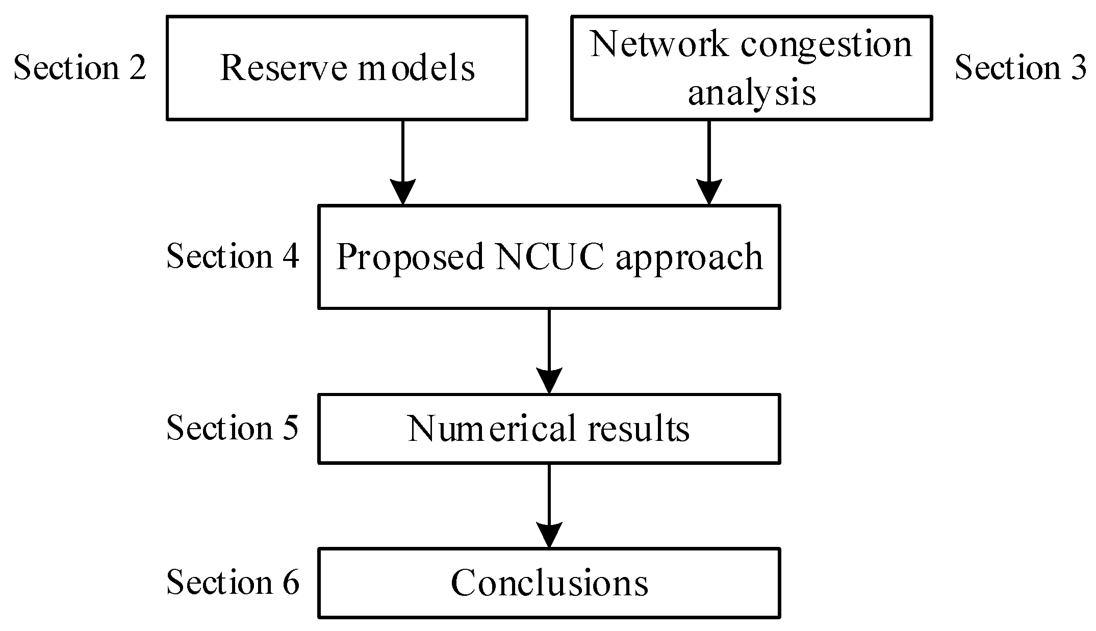
The organization chart of other parts of this paper is shown in Figure 1. Section 2 proposes the reserve models fully considering the stochastic characteristics of wind power. Section 3 analyses the impact of network congestion and proposes the simplified network constraints accordingly. The newly proposed reserve models and simplified network constraints are incorporated into the formulation of the proposed NCUC approach, which is presented in Section 4. Section 5 validated the effectiveness of the proposed approach. Conclusions are drawn in Section 6.

2. Reserve Models Fully Considering Stochastic Characteristics of Wind Power

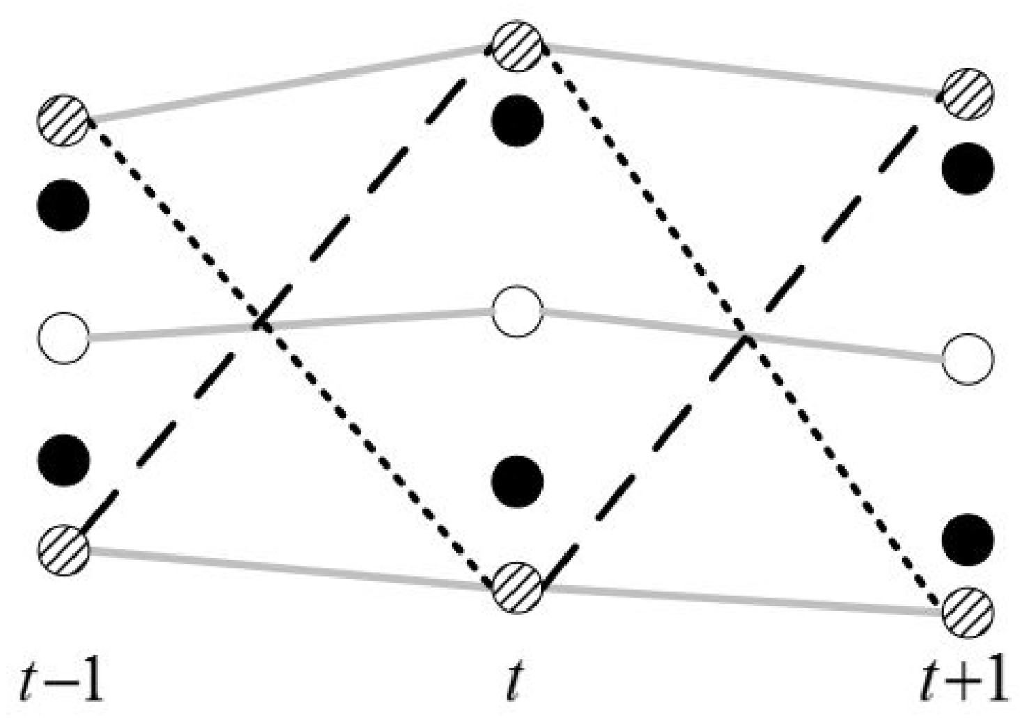
For description convenience, net load, load minus wind power output, is used here to describe the reserve requirements incurred by wind power. The net load change in the consecutive periods can be illustrated in Figure 2, in which the white circles represent the forecasted net load and the shaded circles represent the boundaries of the net load considering the uncertainty. Reserve requirements incurred by net load can be classified into two aspects: one is the reserve requirements incurred by the forecasting errors of net load in a single period; the other is the ramping reserve requirements incurred by the change of net load in two consecutive periods. Correspondingly, reserve optimization consists of two aspects: one is the single-period reserve optimization, which aims to optimize the range of net load that the single-period reserves covers (shown as black circle in Figure 2); the other is the ramping reserve optimization, which aims to optimize the ramping amplitude of net load in two consecutive periods that the ramping reserves covers (the amplitude of ramping up reserve requirements is between zero and the amplitude of the black dashed lines, the amplitude of ramping down reserve requirements is between zero and the amplitude of the black dotted lines, shown in Figure 2).

Reserve models are constructed to implement the above single-period reserve optimization and ramping reserve optimization by reflecting the relationships between the system reserve levels and lost load (or wind power curtailment) caused by reserve shortage. To assess specifically the effect of characteristics of wind power, no uncertain demand and no equipment failure are considered in this paper. Therefore, the change of net load can be recognized to be caused by the stochastic nature of wind power. Reserve models are constructed based on the stochastic characteristics of wind power, which is presented in Section 2.1. Reserve models consist of single-period reserve models and additional ramping reserve models, which are presented in Section 2.2 and Section 2.3, respectively. The linearization of all these reserve models is introduced in Section 2.4.

2.1. Stochastic Characteristics of Wind Power

From the perspective of reserve optimization, the stochastic characteristics of wind power can be classified into two aspects: wind power uncertainty in a single period and wind power change in two consecutive periods. The former one is caused by wind power prediction errors, called single-period wind power characteristics hereinafter. The latter one is affected by the combined effect of wind power prediction errors and wind power variability, also abbreviated as ramping event hereinafter. Wind power stochastic characteristics can be described by the stochastic wind power scenarios tagged with probability information. Wind power scenarios are the time-dependent series of wind power production, including the ramping events as well as the single-period wind power characteristics.

The number of scenarios is a crucial factor that affects the approximation precision of the stochastic characteristics of wind power. Reduced scenarios inevitably discard some stochastic characteristics information of wind power, especially when the adopted scenarios are very few, the loss of stochastic characteristics information is severe. Moreover, reference [28] has verified that scenario reduction techniques fail to concurrently maintain both the single-period wind power characteristics and ramping events.

In order to fully and accurately capture the wind power stochastic characteristics, a sufficiently large number of scenarios are used in the following to construct the reserve models because the number of the adopted scenarios does not affect the complexity of the reserve models. Therefore, reserve models enable the proposed UC approach has a great advantage over SUC that adopts a very limited number of scenarios, in accurately modeling the wind power stochastic characteristics.

Scenario generation method in [29] is applied in this paper to generate the required number of scenarios with equal probability ${\pi }_s=1/\mathrm{S}$ that constitute the scenario set $W=\{W_s,s=1,\cdots ,S\}$, in which $W_s=\{w_{ts},t=1,\cdots ,T\}$. $W_s$ is the sth wind power scenario, $w_{ts}$ is wind power production in period t and scenario s with the probability ${\pi }_{ts}=1/\mathrm{S}$. This scenario generation method accounts for both the interdependence relationship of prediction errors among different periods and the single-period probability distributions of wind power. Therefore, it can well describe both the single-period wind power characteristics and ramping events.

2.2. Single-Period Reserve Models

2.2.1. Single-Period Reserve Requirements

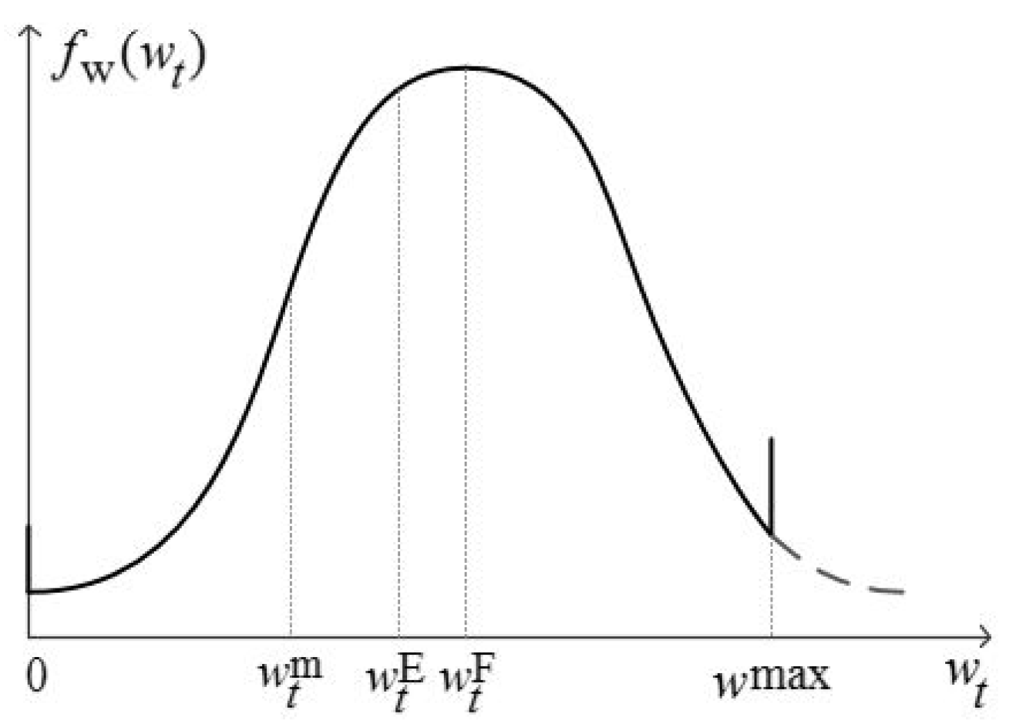
For description convenience, this subsection uses the probability density function (PDF) of wind power production to describe the single-period wind power characteristics. Theoretically, the set constituted by the wind power production of all the scenarios in the same period can be recognized as the discrete approximation of the PDF of wind power production in that period. Without losing generality, the PDF of wind power production can be assumed to accord with some kind of function $f_{\mathrm{w}}(w_t)$, the illustrated diagram of which is shown in Figure 3. Here, wind power production denotes the sum of wind power production at every bus node. The PDF of wind power production in Figure 3 is truncated at the boundaries, the probability density of which is shown in Equation (1), because wind power production should be not less than zero and not greater than the installed capacity $w^{\max }$. In Figure 3, $w_t^{\mathrm{F}}$ and $w_t^{\mathrm{E}}$ represent the point forecast value and the expected value of wind power production. The expected value $w_t^{\mathrm{E}}$ can be expressed as Equation (2), including the integral form and accumulation form:

$$f_{\mathrm{w}}\left(0\right)={\displaystyle {\int }_{-\infty }^0{f}_{\mathrm{w}}\left(w_t\right)d\left(w_t\right)};f_{\mathrm{w}}\left(w^{\max }\right)={\displaystyle {\int }_{w^{\max }}^{+\infty }{f}_{\mathrm{w}}\left(w_t\right)d\left(w_t\right)}$$

(1)

$$w_t^{\mathrm{E}}={\displaystyle {\int }_0^{w^{\max }}{f}_{\mathrm{w}}\left(w_t\right)w_{t}d\left(w_t\right)}={\displaystyle {\sum }_s{\pi }_{ts}{w}_{ts}}$$

(2)

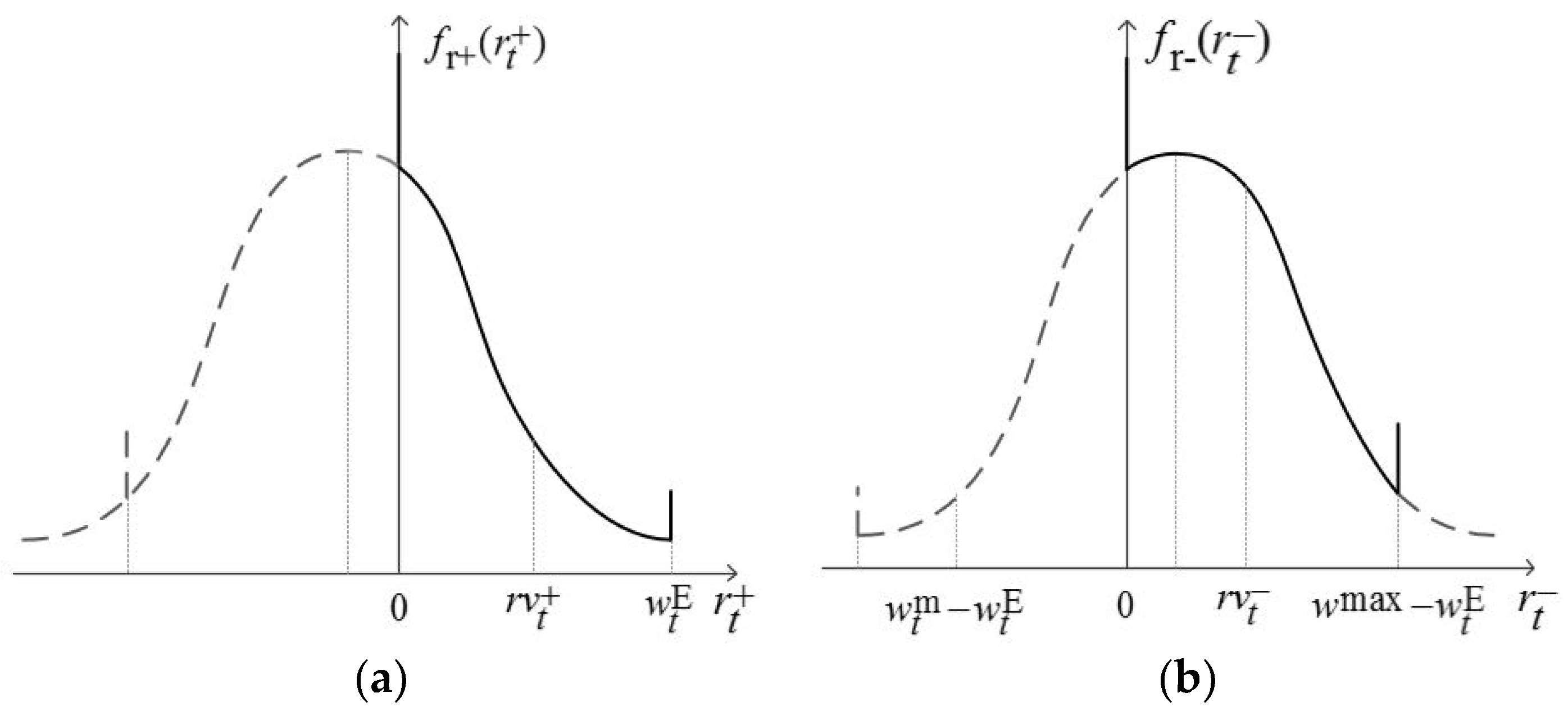
From the viewpoint of a single period, reserve requirements are used to compensate the deviation of actual wind power production from the reference value that is set as $w_t^{\mathrm{E}}$. Single-period up reserve (SPUR) requirements can be recognized as the negative deviation of actual wind power production, i.e., $r_t^{+}=w_t^{\mathrm{E}}-w_t$. Single-period down reserve (SPDR) requirements can be recognized as the positive deviation, i.e., $r_t^{-}=w_t-w_t^{\mathrm{E}}$. The PDFs of the SPUR and SPDR requirements are illustrated in Figure 4a,b. The functions $f_{{\mathrm{r}}^{+}}(r_t^{+})$ and $f_{{\mathrm{r}}^{-}}(r_t^{-})$ should be truncated at their left boundaries because $r_t^{+}\ge 0$ and $r_t^{-}\ge 0$, the probability density of which is amended as Equations (3) and (4), respectively.

$$f_{{\mathrm{r}}^{+}}\left(0\right)={\displaystyle {\int }_{w_t^{\mathrm{E}}}^{w^{\max }}{f}_{\mathrm{w}}\left(w_t\right)d{w}_t}$$

(3)

$$f_{{\mathrm{r}}^{-}}\left(0\right)={\displaystyle {\int }_0^{w_t^{\mathrm{E}}}{f}_{\mathrm{w}}\left(w_t\right)d{w}_t}$$

(4)

2.2.2. Construction of Single-Period Reserve Models

The power system has to shed load when the SPUR requirement $r_t^{+}$ exceeds the given SPUR level $r{v}_t^{+}(0\le r{v}_t^{+}\le w_t^{\mathrm{E}})$, i.e., $r_t^{+}>r{v}_t^{+}$. The expected load not served (ELNS) $r{d}_t^{+}$ caused by SPUR shortage can be expressed as Equation (5), including the integral form and accumulation form. In the accumulation form, the condition $r_t^{+}>r{v}_t^{+}$ is transformed as $w_{ts}\le w_t^{\mathrm{E}}-r{v}_t^{+}$, the symbol $s|w_{ts}\le w_t^{\mathrm{E}}-r{v}_t^{+}$ represents the scenario set that contains all the scenarios that meet the condition $w_{ts}\le w_t^{\mathrm{E}}-r{v}_t^{+}$. This way of representing the scenario set is also adopted hereinafter. Equation (5) denotes the relationship between the SPUR level and the ELNS caused by SPUR shortage, called the SPUR model.

Similarly, the power system has to curtail wind power production when the SPDR requirement $r_t^{-}$ excesses the given SPDR level $r{v}_t^{-}(0\le r{v}_t^{-}\le w^{\max }-w_t^{\mathrm{E}})$, i.e., $r_t^{-}>r{v}_t^{-}$. The expected wind power curtailment (EWC) $r{d}_t^{-}$ caused by SPDR shortage can be expressed as Equation (6). Equation (6) denotes the relationship between the SPDR level and the EWC caused by SPDR shortage, called the SPDR model:

$$r{d}_t^{+}\left(r{v}_t^{+}\right)={\displaystyle {\int }_{r{v}_t^{+}}^{w_t^{\mathrm{E}}}{f}_{{\mathrm{r}}^{+}}\left(r_t^{+}\right)\left(r_t^{+}-r{v}_t^{+}\right)d{r}_t^{+}}={\displaystyle {\sum }_{s|w_{ts}\le w_t^{\mathrm{E}}-r{v}_t^{+}}{\pi }_{ts}\left(w_t^{\mathrm{E}}-r{v}_t^{+}-w_{ts}\right)}$$

(5)

$$r{d}_t^{-}\left(r{v}_t^{-}\right)={\displaystyle {\int }_{r{v}_t^{-}}^{w^{\max }-w_t^{\mathrm{E}}}{f}_{{\mathrm{r}}^{-}}\left(r_t^{-}\right)\left(r_t^{-}-r{v}_t^{-}\right)d{r}_t^{-}}={\displaystyle {\sum }_{s|w_{ts}\ge w_t^{\mathrm{E}}+r{v}_t^{-}}{\pi }_{ts}\left(w_{ts}-w_t^{\mathrm{E}}-r{v}_t^{-}\right)}$$

(6)

Note that the SPDR model may fail to accurately estimate the EWC caused by SPDR shortage if the expected value $w_t^{\mathrm{E}}$ excesses the maximum wind power production $w_t^{\mathrm{m}}$ that the power system can accommodate, i.e., $w_t^{\mathrm{E}}>w_t^{\mathrm{m}}$, shown in Figure 4b. The revisions concerning such a case will be described in detail Section 4.2.3.

2.3. Additional Ramping Reserve Models

Before constructing additional ramping reserve models, we should first recognize that some ramping reserve requirements have already been satisfied through other ways and should be excluded in the construction of additional ramping reserve models to avoid overlapping of the ramping reserves.

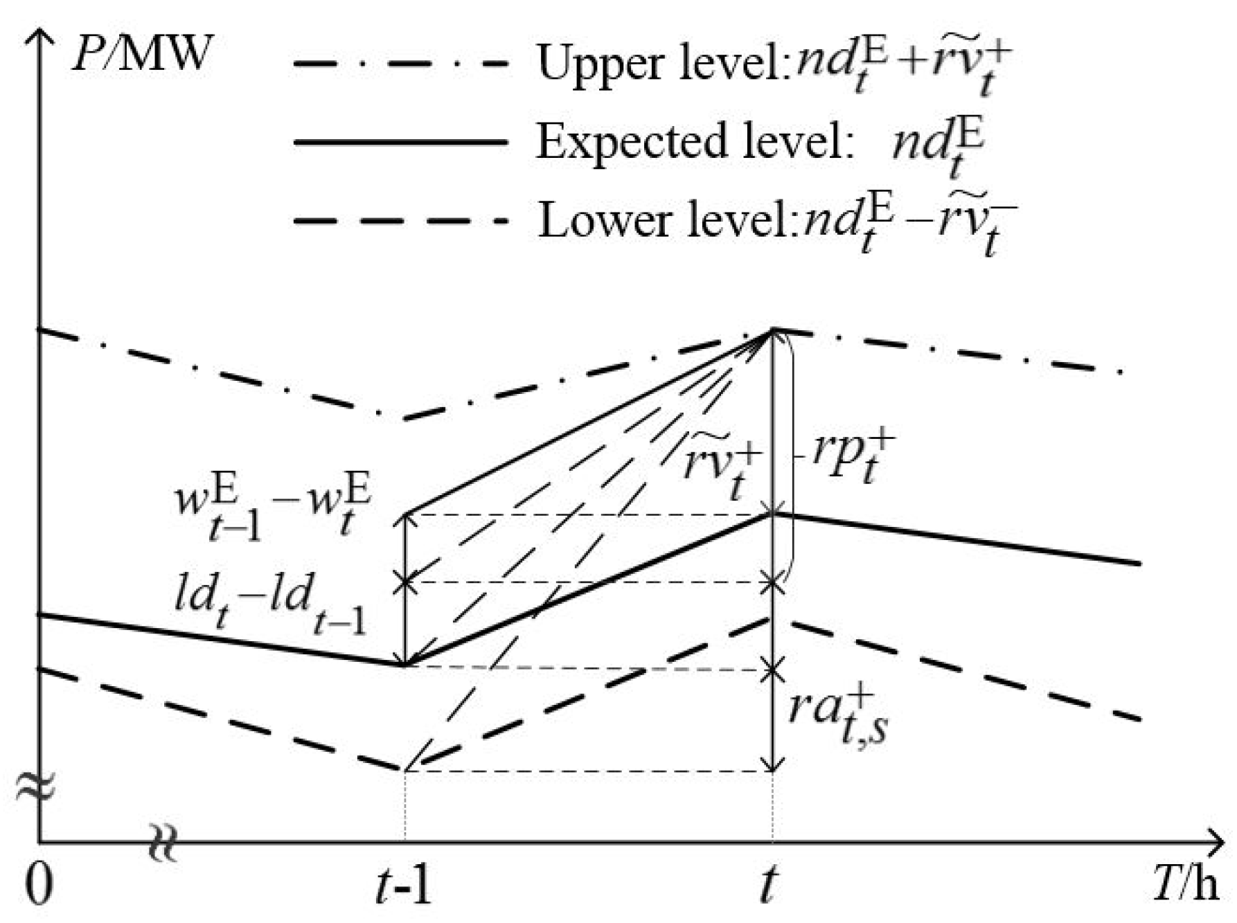
Ramping reserve requirements are caused by the following factors (shown in Figure 5, taking ramping up reserve in two consecutive periods as an example): variation of expected net load ($n{d}_t^{\mathrm{E}}-n{d}_{t-1}^{\mathrm{E}}$), wind power prediction deviation (${\widetilde{rv}}_t^{+}$), and additional ramping reserve requirements ($r{a}_t^{+}$). Ramping reserve requirements caused by expected net load, including load variation ($l{d}_t-l{d}_{t-1}$) and expected wind power variation ($w_{t-1}^{\mathrm{E}}-w_t^{\mathrm{E}}$), can be covered by system power balancing constraint. Ramping reserve requirements caused by wind power prediction deviation can be covered by single-period reserve levels ${\widetilde{rv}}_t^{+},{\widetilde{rv}}_t^{-}$, which should be calculated in advance before constructing the additional ramping reserve models. Additional ramping reserve requirements are used to construct the additional ramping reserve models.

2.3.1. Additional Ramping Reserve Requirements

The existing ramping capacity can cover the expected wind power variation and wind power prediction deviation. Additional ramping reserve requirements can be calculated by subtracting such existing ramping capacity from the actual wind power variation in two consecutive periods (the amplitude of ramping event). The existing ramping up reserve capacity for expected wind power variation and wind power prediction deviation is $r{p}_t^{+}=\max ({\widetilde{rv}}_t^{+},{\widetilde{rv}}_t^{+}+(w_{t-1}^{\mathrm{E}}-w_t^{\mathrm{E}}))$ and the existing ramping down reserve capacity is $r{p}_t^{-}=\max ({\widetilde{rv}}_t^{-},{\widetilde{rv}}_t^{-}+(w_t^{\mathrm{E}}-w_{t-1}^{\mathrm{E}}))$. Then, additional ramping up reserve (ARUR) requirement of scenario $s$ is $r{a}_{ts}^{+}=w_{t-1,s}-w_{ts}-r{p}_t^{+}$ and additional ramping down reserve (ARDR) requirement is $r{a}_{ts}^{-}=w_{ts}-w_{t-1,s}-r{p}_t^{-}$. The value of $r{a}_{ts}^{+},r{a}_{ts}^{-}$ should be set at zero when $w_{t-1,s}-w_{ts}<r{p}_t^{+}$ or $w_{ts}-w_{t-1,s}<r{p}_t^{-}$ because only non-negative additional ramping reserve requirements need to be taken into account.

Additional ramping reserve requirements are calculated after given single-period reserve levels ${\widetilde{rv}}_t^{+},{\widetilde{rv}}_t^{-}$, which can cover the wind power range ${\mathbf{I}}_t^{\mathrm{w}}=[w_t^{\mathrm{E}}-{\widetilde{rv}}_t^{+},w_t^{\mathrm{E}}+{\widetilde{rv}}_t^{-}]$. Because the lost load (or wind power curtailment) caused by wind power scenarios beyond the range ${\mathbf{I}}_t^{\mathrm{w}}$ has been considered in the single-period reserve models, therefore, additional ramping reserve requirements should be limited to the range ${\mathbf{I}}_t^{\mathrm{w}}$ to avoid the repeated calculation of such lost load (or wind power curtailment). For additional ramping reserve requirements, wind power production beyond this range should be adjusted to the corresponding nearer boundaries of the range ${\mathbf{I}}_t^{\mathrm{w}}$. After adjustment, wind power production $w_{ts},w_{t-1,s}$ is rewritten as ${w^{\prime }}_{ts},{w^{\prime }}_{t-1,s}$. Accordingly, the ARUR requirement is rewritten as $r{a}_{ts}^{+}={w^{\prime }}_{t-1,s}-{w^{\prime }}_{ts}-r{p}_t^{+}$ and the ARDR requirement as $r{a}_{ts}^{-}={w^{\prime }}_{ts}-{w^{\prime }}_{t-1,s}-r{p}_t^{-}$.

2.3.2. Construction of Additional Ramping Reserve Models

The power system has to shed load when the ARUR requirement $r{a}_{ts}^{+}$ excesses the given ARUR level $rv{a}_t^{+}$, i.e., $r{a}_{ts}^{+}>rv{a}_t^{+}$. The ELNS $rd{a}_t^{+}$ caused by ARUR shortage can be expressed as Equation (7). Equation (7) denotes the relationship between the ARUR level and the ELNS caused by ARUR shortage, called the ARUR model.

Similarly, the power system has to curtail wind power production when the ARDR requirement $r{a}_{ts}^{-}$ excesses the given ARDR level $rv{a}_t^{-}$, i.e., $r{a}_{ts}^{-}>rv{a}_t^{-}$. The EWC $rd{a}_t^{-}$ caused by ARDR shortage can be expressed as Equation (8). Equation (8) denotes the relationship between the ARDR level and the EWC caused by ARDR shortage, called the ARDR model. Note that ARDR model faces the same problem as the SPDR model when $w_t^{\mathrm{E}}>w_t^{\mathrm{m}}$, which will be solved together in Section 4.2.3:

$$rd{a}_t^{+}\left(rv{a}_t^{+}\right)={\displaystyle {\sum }_{s|r{a}_{ts}^{+}>rv{a}_t^{+}}{\pi }_{ts}\left(r{a}_{ts}^{+}-rv{a}_t^{+}\right)}$$

(7)

$$rd{a}_t^{-}\left(rv{a}_t^{-}\right)={\displaystyle {\sum }_{s|r{a}_{ts}^{-}>rv{a}_t^{-}}{\pi }_{ts}\left(r{a}_{ts}^{-}-rv{a}_t^{-}\right)}$$

(8)

According to the definition of additional ramping reserve requirements, a non-negative additional ramping reserve requirements means that the amplitudes of the corresponding ramping events should excess the corresponding existing ramping capacity, thus, such ramping events have large amplitudes but theoretically low probability. Meanwhile, additional ramping reserve requirements have relatively low value because they are calculated by subtracting the existing ramping capacity from the amplitudes of ramping events. Therefore, additional ramping reserve models constructed based on additional ramping reserve requirements have much less impact on the solutions, compared to the single-period reserve models, and can be regarded as the supplements of the latter ones to further enhance the reliability of the schedule to withstand the risks of both load shedding and wind power curtailment.

2.4. Linearization of Reserve Models

The reserve models in Section 2.2 and Section 2.3 are non-linear and thus are not conducive to being incorporated into the UC formulation. But these models can be linearized by the piecewise linear functions Equations (9) and (10) [30] because they have convex statistical characteristics, illustrated in Figure 6. For simplicity, variables $r{d}_t^{+},r{d}_t^{-},rd{a}_t^{+},rd{a}_t^{-}$ are replaced by variable $r{d}_t$ in Equations (9) and (10), $r{v}_t^{+},r{v}_t^{-},rv{a}_t^{+},rv{a}_t^{-}$ by $r{v}_t$:

$$r{d}_t\left(r{v}_t\right)=r{d}_t\left(0\right)+{\displaystyle {\sum }_k{\alpha }_{tk}\cdot r{v}_{tk}},0\le r{v}_{tk}\le r{v}_t^{\max }/N$$

(9)

$$r{v}_t={\displaystyle {\sum }_{k}r{v}_{tk}}$$

(10)

where $r{v}_{tk}$ is the k-th segment of $r{v}_t$, ${\alpha }_{tk}=(r{d}_t(r{v}_{tk}^{\max })-r{d}_t(r{v}_{t,k-1}^{\max }))\cdot N/r{v}_t^{\max }$, $r{v}_{tk}^{\max }=r{v}_t^{\max }\cdot k/N$, $N$ is the number of the segments.

3. Network Congestion Analysis

The above reserve models focus on the optimization of system reserve levels but neglect that the scheduled reserves may be blocked in real-time operation due to network congestion. In addition, network congestion may not only affect reserve applicability but also occur in the case that has no relationship with reserve applicability, such as the day-ahead schedule under the expected wind power production. Network congestion may result in the increase of real-time operating costs caused by the unexpected lost load or wind power curtailment. However, it is also not an economical choice or even infeasible to avoid such unexpected lost load and wind power curtailment in all the possible wind power scenarios. The ideal remedy is to evaluate the costs/benefits of such lost load (or wind power curtailment) caused by network congestion and to optimize the schedule accordingly. SUC adopts this remedy by introducing many scenario-related network constraints to evaluate the impact of network congestion on the reserve applicability, resulting in heavy computational burden.

To avoid the heavy computational burden caused by many scenario-related network constraints, this section only selects the network constraints (simplified network constraints) that are closely related to network congestion, instead of all the network constraints adopted in the SUC. Further, this section proposes the estimating functions of lost load and wind power curtailment caused by network congestion so that the following UC formulation can evaluate the costs/benefits of such lost load and wind power curtailment.

3.1. Simplified Network Constraints

Evaluating the impact of network congestion needs to resort to the scenario-related network constraints because evaluating reserve applicability should simulate the possible realizations in the real-time operation through stochastic scenarios and because judging network congestion should be on the basis of power flow calculation, which depends on the injected power at every node in the same period and the same scenario. Because the expected wind power production is the expected value of all the stochastic wind power scenarios, scenario-related network constraints can naturally reflect the impact of network congestion on the day-ahead schedule under the expected wind power production.

The network constraints in the SUC needs to contain the power flow constraints of all lines in all periods and scenarios. In the actual power systems that have been well planned, however, network congestion only occurs in a small proportion of periods and wind power scenarios, furthermore, it mainly occurs in a small number of transmission lines. By identifying the set $\mathbf{S}{\mathbf{N}}_{\mathrm{c}}$ of such pairs of period and scenario $(t,s)$ and the set L_c of lines that easily suffer network congestion, only a small number of network constraints are required to reflect the impacts of network congestion on the schedule. The process to obtain such sets will be explained in Section 4.2.2.

The simplified network constraints S_gd include power balance constraint Equation (11), transmission capacity constraint Equation (12), power output constraint of the unit Equation (13), and boundary constraints for load shedding and wind power curtailment Equation (14):

$${\displaystyle {\sum }_i{p}_{its}}={\displaystyle {\sum }_j\left(l{d}_{jt}-w_{jts}-l{s}_{jts}+w{c}_{jts}\right)},\left(t,s\right)\in \mathbf{S}{\mathbf{N}}_{\mathrm{c}}.$$

(11)

$$-p{f}_l^{\max }\le {\mathbf{A}}_l\left({\mathbf{Y}}_{\mathrm{g}}\times {\mathbf{P}}_{ts}+\mathbf{W}{\mathbf{P}}_{ts}-\mathbf{W}{\mathbf{C}}_{ts}-\mathbf{L}{\mathbf{D}}_t-\mathbf{L}{\mathbf{S}}_{ts}\right)=p{f}_{ls}\le p{f}_l^{\max },l\in {\mathbf{L}}_{\mathrm{c}},\left(t,s\right)\in \mathbf{S}{\mathbf{N}}_{\mathrm{c}}.$$

(12)

$$p_{it}-r{g}_{it}^{-}\le p_{its}\le p_{it}+r{g}_{it}^{+},\forall i,\left(t,s\right)\in \mathbf{S}{\mathbf{N}}_{\mathrm{c}}.$$

(13)

$$0\le w{c}_{jts}\le w_{jts},0\le l{s}_{jts}\le l{d}_{jt},\forall j,\left(t,s\right)\in \mathbf{S}{\mathbf{N}}_{\mathrm{c}}.$$

(14)

3.2. Estimating Functions of ELNS and EWC Caused by Network Congestion

Estimating the ELNS and EWC caused by network congestion should exclude the impact of the reserve shortage so as to avoid the overlapping calculation of the ELNS and EWC. Because additional ramping reserves have much less impact compared to single-period reserves, for simplicity, this subsection only considers the impact of the single-period reserves, neglecting that of additional ramping reserves.

The ELNS and EWC caused by network congestion are related to wind power range ${\mathbf{I}}_t^{\mathrm{w}}$. Given the range ${\mathbf{I}}_t^{\mathrm{w}}$, there are two cases, namely, $w_{ts}\in {\mathbf{I}}_t^{\mathrm{w}}$ and $w_{ts}\notin {\mathbf{I}}_t^{\mathrm{w}}$. If $w_{ts}\in {\mathbf{I}}_t^{\mathrm{w}}$, load shedding $l{s}_{ts}^{\mathrm{N}}$ or wind power curtailment $w{c}_{ts}^{\mathrm{N}}$ is solely caused by network congestion. The variable $l{s}_{ts}^{\mathrm{N}}$ is the sum of load shedding $l{s}_{jts}$ at every bus $j$, i.e., $l{s}_{ts}^{\mathrm{N}}={\displaystyle {\sum }_{j}l{s}_{jts}}$, and $w{c}_{ts}^{\mathrm{N}}$ is the sum of wind power curtailment $w{c}_{jts}$ at every bus $j$, i.e., $w{c}_{ts}^{\mathrm{N}}={\displaystyle {\sum }_{j}w{c}_{jts}}$. If $w_{ts}\notin {\mathbf{I}}_t^{\mathrm{w}}$, load shedding or wind spillage is caused by the combined effect of network congestion and single-period reserve shortage. The amount of load shedding caused by reserve shortage can be expressed as $w_t^{\mathrm{E}}-{\widetilde{rv}}_t^{+}-w_{ts}$ and the amount of corresponding wind power curtailment is $w_{ts}-w_t^{\mathrm{E}}-{\widetilde{rv}}_t^{-}$. Then the amount of load shedding caused by network congestion is $l{s}_{ts}^{\mathrm{N}}={\displaystyle {\sum }_{j}l{s}_{jts}}-(w_t^{\mathrm{E}}-{\widetilde{rv}}_t^{+}-w_{ts})$ and the amount of corresponding wind power curtailment is $w{c}_{ts}^{\mathrm{N}}={\displaystyle {\sum }_{j}w{c}_{jts}}-(w_{ts}-w_t^{\mathrm{E}}-{\widetilde{rv}}_t^{-})$.

In addition, the amount of wind power curtailment should be revised when $w_t^{\mathrm{E}}>w_t^{\mathrm{m}}$. In such a case, the amount of wind power curtailment caused by reserve shortage is $w_{ts}-w_t^{\mathrm{m}}$, then the amount of wind power curtailment caused by network congestion is $w{c}_{ts}^{\mathrm{N}}={\displaystyle {\sum }_{j}w{c}_{jts}}-(w_{ts}-w_t^{\mathrm{m}})$.

In conclusion, the ELNS $l{s}_t^{\mathrm{N}}$ caused by network congestion can be expressed as Equation (15) and the EWC $w{c}_t^{\mathrm{N}}$ is Equation (16):

$$l{s}_t^{\mathrm{N}}={\displaystyle {\sum }_{s|w_{ts}\in {\mathbf{I}}_t^{\mathrm{w}}}{\pi }_{ts}l{s}_{ts}}+{\displaystyle {\sum }_{s|w_{ts}\notin {\mathbf{I}}_t^{\mathrm{w}}}{\pi }_{ts}\left[l{s}_{ts}-\left(w_t^{\mathrm{E}}-{\widetilde{rv}}_t^{+}-w_{ts}\right)\right]}$$

(15)

$$w{c}_t^{\mathrm{N}}=s{i}_t{\displaystyle {\sum }_{s|w_{ts}\in {\mathbf{I}}_t^{\mathrm{w}}}{\pi }_{ts}w{c}_{ts}}+s{i}_t{\displaystyle {\sum }_{s|w_{ts}\notin {\mathbf{I}}_t^{\mathrm{w}}}{\pi }_{ts}\left[w{c}_{ts}-\left(w_{ts}-w_t^{\mathrm{E}}-{\widetilde{rv}}_t^{-}\right)\right]}+\left(1-s{i}_t\right){\displaystyle {\sum }_s{\pi }_{ts}\left[w{c}_{ts}-\left(w_{ts}-w_t^{\mathrm{m}}\right)\right]}$$

(16)

where $s{i}_t$ is the auxiliary parameter to indicate the case $w_t^{\mathrm{E}}>w_t^{\mathrm{m}}$, in which it is set at zero, otherwise, $s{i}_t=1$. The method to calculate $s{i}_t$ and $w_t^{\mathrm{m}}$ is provided in Section 4.2.3. The former two items in Equation (16) take effect when $w_t^{\mathrm{m}}\ge w_t^{\mathrm{E}}$ and the last one takes effect when $w_t^{\mathrm{E}}>w_t^{\mathrm{m}}$.

4. NCUC Approach Based on Reserve Models

This proposed NCUC approach introduces the newly proposed reserve models and simplified network constraints into the traditional UC formulation. The reserve models enable this approach to fully capture the impact of the stochastic characteristics of wind power on the reserve optimization and simultaneously optimize the system reserve levels and on/off decision variables. In this way, this approach can comprehensively evaluate the costs and benefits of the scheduled reserves and thus produce very economic schedules. Meanwhile, the reserve models simply consist of a small number of continuous variables and linear constraints and thus bring in very little computational burden. Besides, the simplified network constraints enable this approach to evaluate the impact of network congestion on the schedule at low computational burden. Section 4.1 presents the mathematical formulation of the NCUC based on reserve models (RMUC), Section 4.2 presents the methodology to solve RMUC.

4.1. Mathematical Formulation

The mathematical formulation of RMUC is described as follows:

$$\mathrm{Min}{\displaystyle {\sum }_{i,t}\left[d_t{c}_i\left(p_{it}\right)+c_i^{\mathrm{su}}\left(u_{i,t-1},u_{it}\right)\right]}+{\displaystyle {\sum }_t{d}_{t}v{l}_{t}l{s}_t^{\mathrm{E}}}+{\displaystyle {\sum }_t{d}_{t}v{w}_{t}w{c}_t^{\mathrm{E}}}$$

(17)

$$l{s}_t^{\mathrm{E}}=r{d}_t^{+}+rd{a}_t^{+}+l{s}_t^{\mathrm{N}},\forall t.$$

(18)

$$w{c}_t^{\mathrm{E}}=s{i}_{t}r{d}_t^{-}+s{i}_{t}rd{a}_t^{-}+w{c}_t^{\mathrm{N}},\forall t.$$

(19)

s.t:

$${\displaystyle {\sum }_i{p}_{it}}=l{d}_t-w_t^{\mathrm{E}}+s{w}_t,\forall t.$$

(20)

$${\displaystyle {\sum }_{i}r{g}_{it}^{+}}\ge r{v}_t^{+}+rv{a}_t^{+},\forall t.$$

(21)

$${\displaystyle {\sum }_{i}r{g}_{it}^{-}}\ge r{v}_t^{-}+rv{a}_t^{-},\forall t.$$

(22)

$$p_{it}+r{g}_{it}^{+}\le P_i^{\max }{u}_{it},\forall i,t.$$

(23)

$$p_{it}-r{g}_{it}^{-}\ge P_i^{\min }{u}_{it},\forall i,t.$$

(24)

$$p_{it}-p_{i,t-1}+r{g}_{it}^{+}\le SU{R}_i\left(1-u_{i,t-1}\right)+d_{t}R{U}_i{u}_{i,t-1},\forall i,t.$$

(25)

$$p_{i,t-1}-p_{it}+r{g}_{it}^{-}\le SD{R}_i\left(1-u_{it}\right)+d_{t}R{D}_i{u}_{it},\forall i,t.$$

(26)

$$0\le r{g}_{it}^{+}\le d_{t}R{U}_i,\forall i,t.$$

(27)

$$0\le r{g}_{it}^{-}\le d_{t}R{D}_i,\forall i,t.$$

(28)

$$\left(r{d}_t^{+},r{d}_t^{-}\right)\in {\mathbf{S}}_{\mathrm{rv}}\left(r{v}_t^{+},r{v}_t^{-}\right),\forall t.$$

(29)

$$\left(rd{a}_t^{+},rd{a}_t^{-}\right)\in {\mathbf{S}}_{\mathrm{rva}}\left(rv{a}_t^{+},rv{a}_t^{-}\right),\forall t.$$

(30)

$$\left(p_{its},w_{jts},l{s}_{jts},w{c}_{jts}\right)\in {\mathbf{S}}_{\mathrm{gd}}\left(u_{it},p_{it},r{g}_{it}^{+},r{g}_{it}^{-}\right),\left(t,s\right)\in \mathbf{S}{\mathbf{N}}_{\mathrm{c}}.$$

(31)

The objective function Equation (17) seeks to minimize the total operating costs, including fuel costs, start-up costs, penalty costs of ELNS, and penalty costs of EWC. Fuel cost functions are usually expressed as quadratic functions, which are approximated by the piecewise linear functions [30]. Start-up cost functions are the functions of commitment variables, in which the start-up cost of each time is set to constant [17]. Equations (18) and (19) are used to calculate the total ELNS and the total EWC, respectively, both of which contain three parts and are caused by three factors: the single-period reserve shortage, additional ramping reserve shortage, and network congestion. Equation (19) also introduces parameter $s{i}_t$ to identify the case $w_t^{\mathrm{E}}>w_t^{\mathrm{m}}$ as Equation (16) does. When $w_t^{\mathrm{E}}>w_t^{\mathrm{m}}$, the EWC caused by the single-period reserve shortage and the additional ramping reserve shortage is excluded through setting $s{i}_t=0$ to avoid the overlapping calculation of such EWC. More detail about the revision of EWC will be explained in Section 4.2.3. Note that parameters $v{l}_t,v{w}_t$ are not predefined and are calculated according to the operating costs in each period. The calculations of $v{l}_t,v{w}_t$ are explained in Section 4.2.2.

Note that the penalty costs of ELNS and EWC in the objective function Equation (17) is quite different from those in the objective function of DUC due to their different calculations of load shedding and wind power curtailment. Traditional DUC can only consider the load shedding and wind power curtailment under the expected (or point forecasted) wind power scenario. But the ELNS and EWC in the objective function Equation (17) represent the total expected load shedding and the total expected wind power curtailment, respectively, caused by both reserve shortage and network congestion. In this way, the penalty costs of ELNS and EWC in the objective function Equation (17) can be used to express the potential benefits of both the scheduled reserves and mitigating network congestion, or in more straightforward words, the potentially reduced penalty costs of ELNS and EWC due to both the scheduled reserves and mitigating network congestion. The increased costs of both the scheduled reserves and mitigating network congestion can be calculated by the former two terms of objective function Equation (17), i.e., fuel costs and start-up costs. Therefore, objective Equation (17) can comprehensively evaluate the costs and benefits of both the scheduled reserves and eliminating network congestion, but the objective in the DUC is incapable of doing that.

RMUC is restricted by the following constraints: power balance constraint Equation (20), system up and down spinning reserve requirements Equations (21) and (22), upper and lower power limits of the unit Equations (23) and (24), ramping up and down reserve limits of the unit Equations (25) and (26), reserve boundaries of the unit Equations (27) and (28), single-period reserve models Equation (29), additional ramping reserve models Equation (30), and simplified network constraints Equation (31). Constraint Equation (20) introduces the slack variable $s{w}_t$ to attain the feasibility of the model when the case $w_t^{\mathrm{E}}>w_t^{\mathrm{m}}$ occurs. Constraints Equations (21) and (22) regard system up and down spinning reserve requirements as decision variables, which are correlated to the ELNS Equation (18) and EWC Equation (19) through reserve models Equations (29) and (30) and thus can be optimized based on the cost/benefit analysis. Single-period reserve models Equation (29) consist of Equations (5) and (6). Additional ramping reserve models Equation (30) consist of Equations (7) and (8). The single-period reserve capacity and additional ramping reserve capacity are deployed as the spinning reserves in this paper, for simplicity, temporarily neglecting the non-spinning reserves. Simplified network constraints Equation (31) consist of Equations (11)–(14). In addition, RMUC includes other technique constraints such as minimum up- and down-time limits, which are not provided in this paper for the sake of brevity and can be referred to [31].

It is important to emphasize that there are two remarkable aspects of differences between the RMUC and typical DUC [6], despite the fact they both follow the traditional UC framework to achieve high computational efficiency. On the one hand, system up and down spinning reserve requirements are decision variables in the RMUC, instead of the predefined value in the DUC. Similar to SUC, RMUC can evaluate the costs and benefits of the system spinning reserve requirements and thus produce very economical reserve strategy. On the other hand, RMUC can evaluate the impact of network congestion on the reserve applicability through the network constraints Equation (31). But typical DUC simply considers the network constraints under the expected (or point forecasted) wind power scenario and thus fails to consider that the scheduled reserves may be blocked in the real-time operation due to network congestion.

4.2. Methodology of Solving RMUC

The methodology of solving RMUC is illustrated in Figure 7. RMUC requires some essential parameters such as ${\mathbf{I}}_t^{\mathrm{w}}$, $\mathbf{S}{\mathbf{N}}_{\mathrm{c}}$, and ${\mathbf{L}}_{\mathrm{c}}$, which should be calculated in advance. Initial UC (IUC) provides the parameter ${\mathbf{I}}_t^{\mathrm{w}}$ and also provides the initial schedule for economic dispatch (ED) simulations. ED simulations can simulate the real-time operation to provide some other required parameters such as $\mathbf{S}{\mathbf{N}}_{\mathrm{c}}$ and ${\mathbf{L}}_{\mathrm{c}}$.

4.2.1. Solving IUC

Compared to RMUC, IUC does not contain additional ramping reserve model Equation (30) and network constraints Equation (31) and should replace Equations (18) and (19), Equations (21) and (22) by Equations (32)–(35). Parameters $v{l}_t,v{w}_t$ in the IUC are taken as the empirical value. IUC is simple and quite computationally efficient. After solving IUC, the wind power range ${\mathbf{I}}_t^{\mathrm{w}}$ can be obtained according to $r{v}_t^{+},r{v}_t^{-}$:

$$l{s}_t^{\mathrm{E}}=r{d}_t^{+},\forall t.$$

(32)

$$w{c}_t^{\mathrm{E}}=r{d}_t^{-},\forall t.$$

(33)

$${\displaystyle {\sum }_{i}r{g}_{it}^{+}}\ge r{v}_t^{+},\forall t.$$

(34)

$${\displaystyle {\sum }_{i}r{g}_{it}^{-}}\ge r{v}_t^{-},\forall t.$$

(35)

4.2.2. ED Simulations

ED simulations can simulate the possible realizations of real-time operation through stochastic scenarios to analyze the possible impact of network congestion on the schedule and to estimate the expected operating costs regarding all the possible realizations. Each ED model in the ED simulations corresponds to one stochastic scenario and can be regarded as the SUC model under a single scenario with the given commitment decision variables provided by IUC. The ED model is a linear programming problem that is quite computationally efficient. Besides, ED models under different scenarios are mutually independent and thus can be paralleled solved to further improve the computational efficiency.

ED simulations can assess the impact of network congestion on the schedule and thus obtain the parameters $\mathbf{S}{\mathbf{N}}_{\mathrm{c}}$ and ${\mathbf{L}}_{\mathrm{c}}$. In ED simulations, if there is any pair of scenario and period in which the lost load (or wind power curtailment) caused by network congestion satisfies the condition $l{s}_{ts}^{\mathrm{N}}>0$ (or $w{c}_{ts}^{\mathrm{N}}>0$), such pair of scenario and period will be included into the set $\mathbf{S}{\mathbf{N}}_{\mathrm{c}}$. The functions to calculate the value $l{s}_{ts}^{\mathrm{N}},w{c}_{ts}^{\mathrm{N}}$ can be referred to Section 3.2, the required variables in these functions can be approximately obtained by the corresponding data from the solutions of the IUC and ED simulations. In ED simulations, if any transmission reaches its transmission capacity, such line will be included into the set ${\mathbf{L}}_{\mathrm{c}}$.

Besides, ED simulations can calculate the expected operating costs regarding all the scenarios in every period and thus can calculate the parameters $v{l}_t,v{w}_t$. The value of loss load $v{l}_t$ is set at the fixed times of the operating costs per load demand in period $t$. The value of wind power curtailment $v{w}_t$ is set at the operating costs per net load (load minus wind power) in period $t$, representing the opportunity costs of curtailed wind power.

However, ED simulations cannot adopt as many scenarios as reserve models do because too many scenarios in ED simulations may lead to that the scale of the set $\mathbf{S}{\mathbf{N}}_{\mathrm{c}}$ is too large when the network is heavily congested. Though the set $\mathbf{S}{\mathbf{N}}_{\mathrm{c}}$ accounts for a small proportion of all the pairs of period and scenario considered in the SUC, its proportion still rises with the aggravation of network congestion, moreover, the scale of the set $\mathbf{S}{\mathbf{N}}_{\mathrm{c}}$ is proportional to the number of scenarios. A large set $\mathbf{S}{\mathbf{N}}_{\mathrm{c}}$ impairs the computational efficiency of RMUC, therefore, ED simulations should reduce the scenarios of the set $\mathbf{W}$ adopted in reserve models. The k-means clustering technique is applied in this paper to reduce the scenarios [28].

4.2.3. Solving RMUC

Besides the parameters mentioned in the above two processes, the parameters $s{i}_t$ and $w_t^{\mathrm{m}}$ should also be calculated in advance before solving RMUC. The parameter $s{i}_t$ is used to identify the case $w_t^{\mathrm{E}}>w_t^{\mathrm{m}}$, in which the EWC caused by reserve shortage can be roughly approximated by $w_t^{\mathrm{E}}-w_t^{\mathrm{m}}$, i.e., the value of $s{w}_t$ in the power system balance constraint Equation (20). This approximation of EWC is not accurate but has little impact on the economy of the schedule due to the low value of wind power curtailment. In such a case, the EWC caused by the single-period reserve shortage and additional ramping reserve shortage has been included in the system power balance constraint Equation (20) and therefore Equation (19) need to exclude such EWC by setting $s{i}_t=0$. Because $w_t^{\mathrm{E}}-w_t^{\mathrm{m}}$ is equal to $s{w}_t$, $s{i}_t$ can be approximated by value of $s{w}_t$ ($s{w}_t^0$) in the IUC. When $s{w}_t^0>0$, $s{i}_t$ is set at zero and $w_t^{\mathrm{m}}$ is $w_t^{\mathrm{E}}-s{w}_t^0$, otherwise, $s{i}_t$ is set at one and $w_t^{\mathrm{m}}$ is zero. After solving RMUC, the EWC can be calculated by Equation (36):

$$w{c}_t^{\mathrm{E}}=s{i}_{t}r{d}_t^{-}+s{i}_{t}rd{a}_t^{-}+\left(1-s{i}_t\right)s{w}_t+w{c}_t^{\mathrm{N}},\forall t.$$

(36)

The above processes provide a simple way for RMUC to calculate its required parameters, which may slightly depart from their optimal value. However, the above processes can provide a good approximation of the core parameters, including ${\mathbf{I}}_t^{\mathrm{w}}$, ${\mathbf{L}}_{\mathrm{c}}$, and $\mathbf{S}{\mathbf{N}}_{\mathrm{c}}$. The parameter ${\mathbf{I}}_t^{\mathrm{w}}$ mainly affects the additional ramping reserve models, which are the supplements of single-period reserve models and have much less impact on the schedule compared to single-period reserve models. The parameters ${\mathbf{L}}_{\mathrm{c}}$ and $\mathbf{S}{\mathbf{N}}_{\mathrm{c}}$ are used to manage the possible network congestion and will not vary apparently if the set ${\mathbf{L}}_{\mathrm{c}}$ is carefully selected. The set ${\mathbf{L}}_{\mathrm{c}}$ can be well selected by ED simulations and can be better selected with the help of historical operation data.

5. Numerical Results

Numerical simulations use the modified version of 118-bus test system from motor.ece.iit.edu/data/ltscuc, so as to better accord with the engineering practice. The modified system consists of 54 units with a total installed capacity of 14,470 MW and with the peak load of 13,000 MW. Ten wind farms are integrated into the modified system at ten different bus nodes, each with 450 MW of installed capacity. Wind data are from [32]. The initial value of wind power curtailment is 40 $/MW∙h for the IUC. The value of lost load is fixed at 1000 $/MW∙h for the sake of comparisons among different UC approaches. Ten-piece piecewise linear functions are used to approximate the fuel cost functions, fifty-piece piecewise linear functions to approximate the single-period reserve models, and ten-piece piecewise linear functions to approximate the additional ramping reserve models.

All numerical simulations are coded with YALMIP toolbox under the MATLAB platform and are solved by the commercial solver GUROBI 6.0.5 with a pre-specified optimal gap of 0.1% on a Windows-based server equipped with a Xeon ES-1650 (3.50 GHz, six6 cores) processor. The simulation results are presented in the following two parts: Section 5.1 compares the economic performance of schedules produced by different approaches, including DUC, SUC, and RMUC; Section 5.2 compares their computing performance.

5.1. Economic Performance Analysis

DUC is represented by the traditional 3σ approach, which sets the system up reserve level as three times the standard deviation (3σ) of the wind power forecasting errors. The SUC formulation used for comparison is derived from [19]. Three thousand (3000) scenarios, which constitute the original scenario set $\mathbf{W}$, are generated by the method in [29] to fully approximate the stochastic characteristic of wind power. The original scenario set is used to construct the reserve models and then is reduced to a small scenario set containing 20 scenarios by the k-means clustering method [28]. The reduced scenario set is used in the SUC and in the ED simulations of RMUC. More scenarios adopted in the reduced scenario set may contribute to the better economic performance of SUC, but more scenarios require so many computational resources that are beyond the ability of our simulation environment.

The day-ahead schedules directly produced by different UC approaches are not comparable because these approaches adopt different means of modeling wind power characteristics. But these approaches can be compared when their day-ahead schedules have been implemented real-time simulations, i.e., ED simulations under the original scenario set ${\mathbf{W}}_t$. Economic performance results of the three different approaches are provided in

Table 1. Economic performance results of three approaches.

Approach	TOC/$ 1 M		TFC/$ 1M		ELNS/MW·h		EWC/MW·h
	RT	Δ	RT	Δ	RT	Δ	RT	Δ
DUC_1.0	8.237	0.337	7.740	0.080	258	256	6856	399
SUC_1.0	8.204	0.228	7.764	0.033	204	195	6856	160
RMUC_1.0	8.096	0.006	7.823	0.047	35	−1	8308	88
DUC_1.2	8.261	0.358	7.743	0.082	278	277	6891	434
SUC_1.2	8.218	0.234	7.764	0.032	218	202	6888	153
RMUC_1.2	8.093	0.003	7.822	0.041	21	−10	8104	86
DUC_1.4	8.380	0.460	7.758	0.078	382	382	6798	543
SUC_1.4	8.213	0.184	7.819	0.031	159	153	8232	125
RMUC_1.4	8.153	0.034	7.843	0.052	52	9	8231	69

, including total operating costs (TOC), total fuel costs (TFC), expected load not served (ELNS), and expected wind power curtailment (EWC). The column RT represents the real-time expected results calculated by the results of real-time simulations, Δ represents the difference between the real-time expected results and the day-ahead schedule results. Moreover, Table 1 gives the results of the three approaches under different severity degrees of network congestion. The suffixes (1.0, 1.2, and 1.4) in the first column are congestion factors $\rho$, which are used to represent the severity degree of network congestion. Assuming the initial transmission capacity of line $l$ is $p{f}_l^{\max }$, then the transmission capacity of the corresponding line for the test system with the congestion factor $\rho$ is $p{f}_l^{\max }/\rho$. The congestion factor is larger, there are more lines that are prone to congestion.

As shown in Table 1, RMUC has the lowest total operating costs compared to DUC and SUC, furthermore, has the lowest differences (Δ) regarding the two most important indexes, i.e., the total operating costs and the ELNS. The penalty costs of ELNS greatly affect the total operating costs because the value of lost load is very high. Therefore, accurately estimating the ELNS in the day-ahead schedule is crucial for the economic performance of a UC approach. DUC and SUC heavily underestimate the ELNS in the day-ahead schedule, resulting in the remarkable increase of total operating costs in the real-time expected results. Instead, RMUC can better estimate the ELNS in the day-ahead schedule and thus produce more economical schedule.

On the other hand, RMUC is much less sensitive to the severity degree of network congestion compared to DUC. This is because DUC ignores the impact of network congestion on the reserve applicability. If the network congestion aggravates, the economic performance of DUC worsens. When the congestion factor is $\rho =1.4$, DUC needs the more total operating costs by 1.99% and 2.71% compared to SUC and RMUC.

5.2. Computing Performance Analysis

The number of variables and the number of constraints are the important and intuitional indexes that reflect the model scale of the UC approach. The model scale remarkably affects the computing time of the UC approach, however, computing time is also affected by other complex factors such as the algorithm. The impact of the algorithm on the computing time is complicated and is beyond the scope of this paper. All the formulations of these three UC approaches are solved by the same commercial MILP solver of GUROBI in this paper.

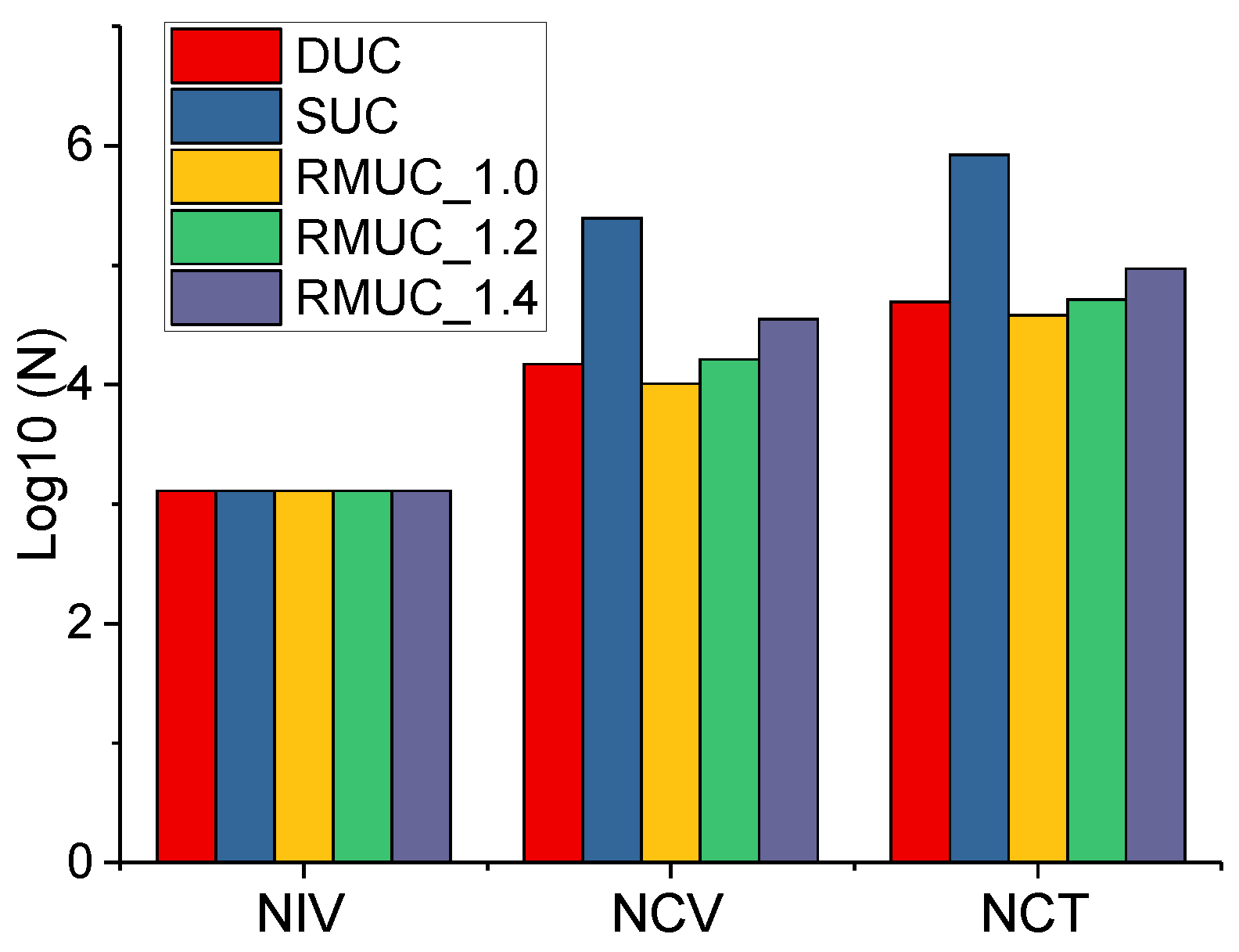
The model scales of different approaches are shown in Figure 8, including the number of integer variables (NIV), the number of continuous variables (NCV), the number of constraints (NCT). The values of these indexes are written in the form of logarithm. Note that the model scales of DUC and SUC have no relationship with the severity degree of network congestion so they have no suffixes indicating the severity degree of network congestion in Figure 8. The computing performance of different approaches is illustrated in

Table 2. Computing performance of different approaches.

Approach	NSP	NL	CPT(s)
DUC_1.0	24	186	44
SUC_1.0	480	186	2410
RMUC_1.0	4	3	28
DUC_1.2	24	186	24
SUC_1.2	480	186	2676
RMUC_1.2	43	11	29
DUC_1.4	24	186	37
SUC_1.4	480	186	6594
RMUC_1.4	165	15	118

, including the number of the pairs of scenario and period (NSP), the number of lines (NL), and computing time (CPT).

As shown in Figure 8, RMUC has much smaller model scale compared to SUC especially when the network congestion is slight. The model scale of RMUC increases when the congestion factor enlarges, but even when $\rho =1.4$, the number of continuous variables of RMUC is only 1/7 of that of SUC and the number of constraints is only 1/9. The advantage of RMUC in the model scale over SUC attributes to that RMUC can pick out the scenarios, periods, and lines that are easily suffered to network congestion and thus has much smaller NSP and NL, which is verified in Table 2, avoiding many inactive constraints adopted in the SUC. Therefore, RMUC has a more reasonable model scale that varies depending on the severity degree of network congestion, compared to SUC.

When $\rho =1.0$ or $\rho =1.2$, RMUC has the similar computing time as DUC and has much less computing time compared to SUC. When $\rho =1.4$, RMUC consumes a little more computing time compared to DUC. It is important to note that the SUC consumes much more time when $\rho =1.4$ compared to when $\rho =1.0$ though the model scale keeps the same. This is because more network constraints take effect when the network congestion aggravates. When $\rho =1.4$, the computing time of RMUC is only 1/56 of that of SUC.

6. Conclusions

This paper proposes a new NCUC approach that introduces the newly proposed reserve models and simplified network constraints. This approach constructs the reserve models based on a sufficiently large number of stochastic wind power scenarios to fully and accurately capture the stochastic characteristics of wind power. These reserve models are directly incorporated into traditional UC formulation to simultaneously optimize the system reserve levels and on/off decision variables. Therefore, the proposed approach can better perform the cost/benefit analysis in the reserve optimization and thus produce very economical schedule. These reserve models bring in very little computational burden because they simply consist of a small number of continuous variables and linear constraints. Besides, this approach can reflect the impact of network congestion on the schedule by introducing only a small number of network constraints, i.e., the simplified network constraints, and thus can concurrently ensure its high computational efficiency.

Numerical simulations have been performed to compare the economic performance and computing performance of DUC, SUC, and RMUC. The following conclusions can be drawn accordingly:

(1)

RMUC can better estimate the real-time expected results, containing total operating costs and expected load not served, in the day-ahead schedule compared to DUC and SUC. However, DUC and SUC fail to accurately estimate the expected load not served in the day-ahead schedule, resulting in the remarkable increase of total operating costs in the real-time simulations.

(2)

RMUC can produce more economical schedule compared to DUC and SUC and effectively cope with the impact of network congestion on the schedule. When the network congestion aggravates, RMUC has much more advantage in economic performance over DUC.

(3)

RMUC is much more computationally efficient than SUC and has similar computational efficiency as DUC. This is partly because RMUC has a more reasonable model scale that varies depending on the severity degree of network congestion, compared to SUC, avoiding many inactive constraints adopted in the SUC.

This proposed approach focuses on the spinning reserves and neglects the non-spinning reserves. The extension of this approach should be further studied to make it more widely applicable.