Risk Assessment of Power System Considering Frequency Dynamics and Cascading Process

School of Electrical Engineering, Wuhan University, Wuhan 430072, China
*
Author to whom correspondence should be addressed.
†
Current address: No. 8 South Street of East Lake, Wuhan 430072, China.
Energies 2018, 11(2), 422; https://doi.org/10.3390/en11020422
Submission received: 7 December 2017
/
Revised: 24 January 2018
/
Accepted: 25 January 2018
/
Published: 12 February 2018
(This article belongs to the Section F: Electrical Engineering)
Abstract
:Frequency security is vital to the safety of power systems and has been scrutinized for many years. The conventional frequency security analysis only checks whether the frequency after anticipated initial failures can remain in the normal range based on some aggregated models, but the influence of potential cascading failures has not been considered yet. This is not enough, especially when the modern power system suffers the increasing threat of cascading failures. Therefore, this paper proposes a novel frequency simulation model considering the influence of cascading failure to reveal the security level of power systems comprehensively. The proposed model is based on a platform on which the frequency dynamics and the power flow distributions can be calculated jointly. Moreover, simulation models of protection devices and some supervisory operation-control schemes are also taken into account. Case studies validate the effectiveness of the proposed model on the IEEE 39-bus system. Moreover, the results of some further probabilistic simulations under different operation parameters are obtained, which show the great significance of improving the frequency regulation performance to cope with challenges of blackouts.
1. Introduction
Frequency security has been the focus of power system operation for a long time. As an effective reflection of active power balance, frequency should be maintained within a specific range to ensure the uninterrupted working of electrical elements. Otherwise, many frequency-related protection devices may be triggered and then result in severe consequences.
The modern power system keeps advancing towards a huge complex artificial system. Interactions among electrical elements become rather sophisticated, such that even a simple disturbance can trigger the chain reaction of the whole system known as the “cascading failure”, which is the main cause of power blackouts [1,2]. The element outages and the unplanned system splitting appearing in the spreading of cascading failure may bring great power mismatch. If not dealt with correctly, this power mismatch will lead to frequency insecurity, which may further cause massive loss of load and generation, or even system collapse. Thus, it can be inferred that the frequency dynamic plays an important role in the process of cascading failure.
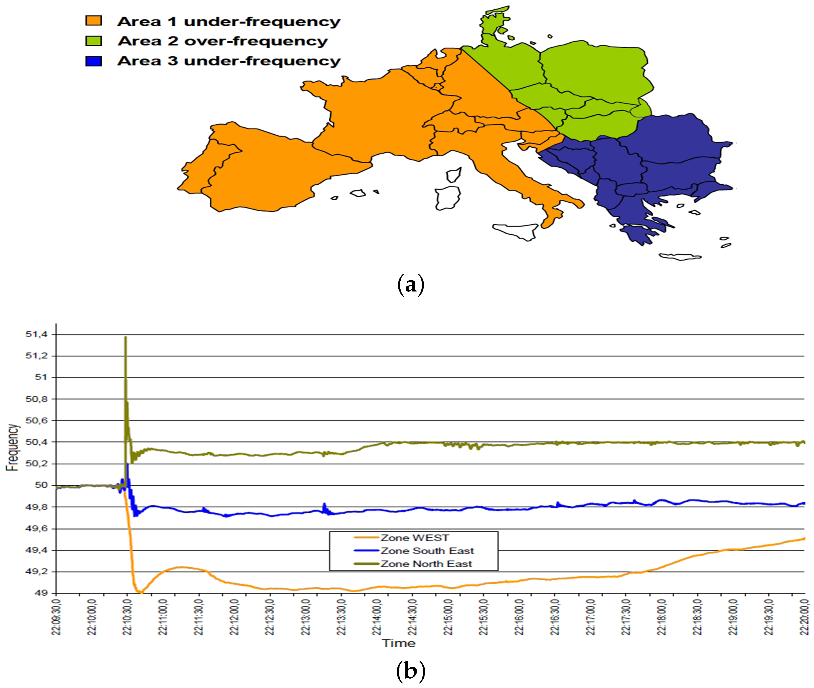
In fact, the aforementioned discussion can be validated by the historical records of blackouts worldwide. Figure 1 depicts the frequency dynamics during the blackout that occurred in Europe on 4 November 2006 [3]. The interconnected European electric grid split into three independent parts unexpectedly due to the successive outages of overloaded lines. As shown in Figure 1, the frequency of Area 1 dropped quickly to about 49 Hz, resulting in load shedding of about 17,000 MW. In the meantime, the frequency of Area 2 rose quickly to about 51.4 Hz due to the severe power surplus of over 10,000 MW. Finally, it was restored to 50.3 Hz with the measures of primary frequency control and active generator tripping. Area 3 also underwent an under-frequency situation leading to a large amount of load shedding. Fortunately, all of these three areas maintained the frequency security with several emergency measures. However, if the system was in inappropriate operation conditions, for example, incorrect allocation of spinning capacity or ill-fitted parameter settings of under-frequency load-shedding (UFLS) schemes, the subgrids would be at risk of complete collapse. Such cases can be found in many blackouts, including the one on 30 July 2012 in India, the one on 8 August 1996 in Malaysia [4] and the one on 10 November 2009 in Brazil [5].
In fact, for those free-connected power grids that do not have apparent hierarchical or zoned structures, the spreading of cascading failures is highly likely to result in unexpected splitting of the grid. This dynamic process may not be examined when planning the operation conditions or setting the parameters of frequency-related protection devices. Thereby, there are still two major problems in the face of such frequency-related outages:
- Model building: The existing frequency-simulation models are not suitable for the security assessment considering cascading failure process. Full time-transient simulation models can provide an accurate estimation of frequency dynamics, but they are time-consuming and sometimes cannot highlight the influence of frequency security when rotor and voltage stabilities are considered. Thus, some dedicated simplified models were built to reduce the computational burden, including the system frequency response (SFR) model [6] and the average system frequency (ASF) model [7] shown in Figure 2. The SFR model averages all generators into an single equivalent generator, and the ASF model reserves the governor model of individual generators so as to reveal their regulation discrepancy. However, both of them neglect the structure of the power system. They can not simulate the dynamics when branch outages and unexpected system splitting occurs.
- Analysis paradigm: The conventional paradigm of frequency security analysis only investigates whether the frequency after N-1 or N-2 contingencies can remain within a secure range. Firstly, it does not take into account the influence of cascading events. Some potentially severe situations may be thus excluded. Secondly, the conventional paradigm is mostly based on deterministic analysis. However, there are many random factors in the dynamic process of power systems [8,9]. Thus, a statistical method should be introduced to assess the security level more comprehensively. Ref. [10] utilized the SFR model to investigate the power-law distribution of load loss considering cascading generator outages. However, the influence of power-grid structure was not taken into account as well.
In addition, the modeling and analysis of cascading failures also need to integrate the depiction of frequency dynamics. Some static power-flow-based cascading failure models, for example, the ORNL-PSerc-Alaska (OPA) model [11], the Manchester model [12] and the improved OPA model [8], cannot simulate the frequency dynamics and deal with the power mismatch in simple ways. Recently, some full-time transient simulation-embedded models were proposed by [13,14,15]. They can simulate the detailed dynamics of the cascading process, but their computations are relatively slow, and some important supervisory control measures are not considered, for example, frequency-related generator tripping and emergency dispatch (ED) scheme. Thus, combination of the comprehensive modeling of frequency dynamics and the cascading failure simulation is meaningful and may bring more insightful discoveries about the blackouts.
Ref. [16] proposed a novel direct current (DC) power-flow-based frequency response model, abbreviated as DFR, which artfully combines a dynamic model of a single generator [16], a simplified load model considering frequency dependency, and DC power-flow equations of a power grid. It offers a platform to simultaneously calculate the frequency dynamics and power-flow distribution jointly. However, the original DFR model in [16] only investigated frequency security after a single outage of a generator or branch. It could be introduced to assess the frequency security under cascading failure. Thus, we regard the DFR model as the foundation of our further research and propose a comprehensive frequency-security simulation model. The proposed model considers several factors that may propagate the cascading failure, for example, overloading protection of branches (OPB), abnormal frequency protection of generators (AFPG), UFLS, active over-frequency tripping of generators and ED. The corresponding calculation framework and model validation will also be presented. Moreover, statistical assessments are carried out not only under random initial outages with different severities, but also with different operation parameters. Probabilistic indexes are proposed to reveal the system security level including average ratio of frequency-insecurity-induced load loss, conditional value at risk, and so on.
It is noted that the adoption of a DC load-flow model is a limitation, since some other issues involved in the power system security are not considered, for example, the rotor/voltage/small-signal instability. Thus, instead of being used to reproduce the cascading sequences to approximate the real blackout records, the proposed model is more recommended to reveal the frequency-stability-related statistical features of power grids under cascading failures.
The rest of this paper is organized as follows. In Section 2, specifics of the proposed model are offered. In Section 2, model validation is also presented. Then, case studies on the IEEE 39-bus benchmark are demonstrated in Section 3. Finally, conclusions are drawn in Section 4, where the future work is also discussed.
2. Frequency-Simulation Model Considering Cascading Failure Process
2.1. DFR Model
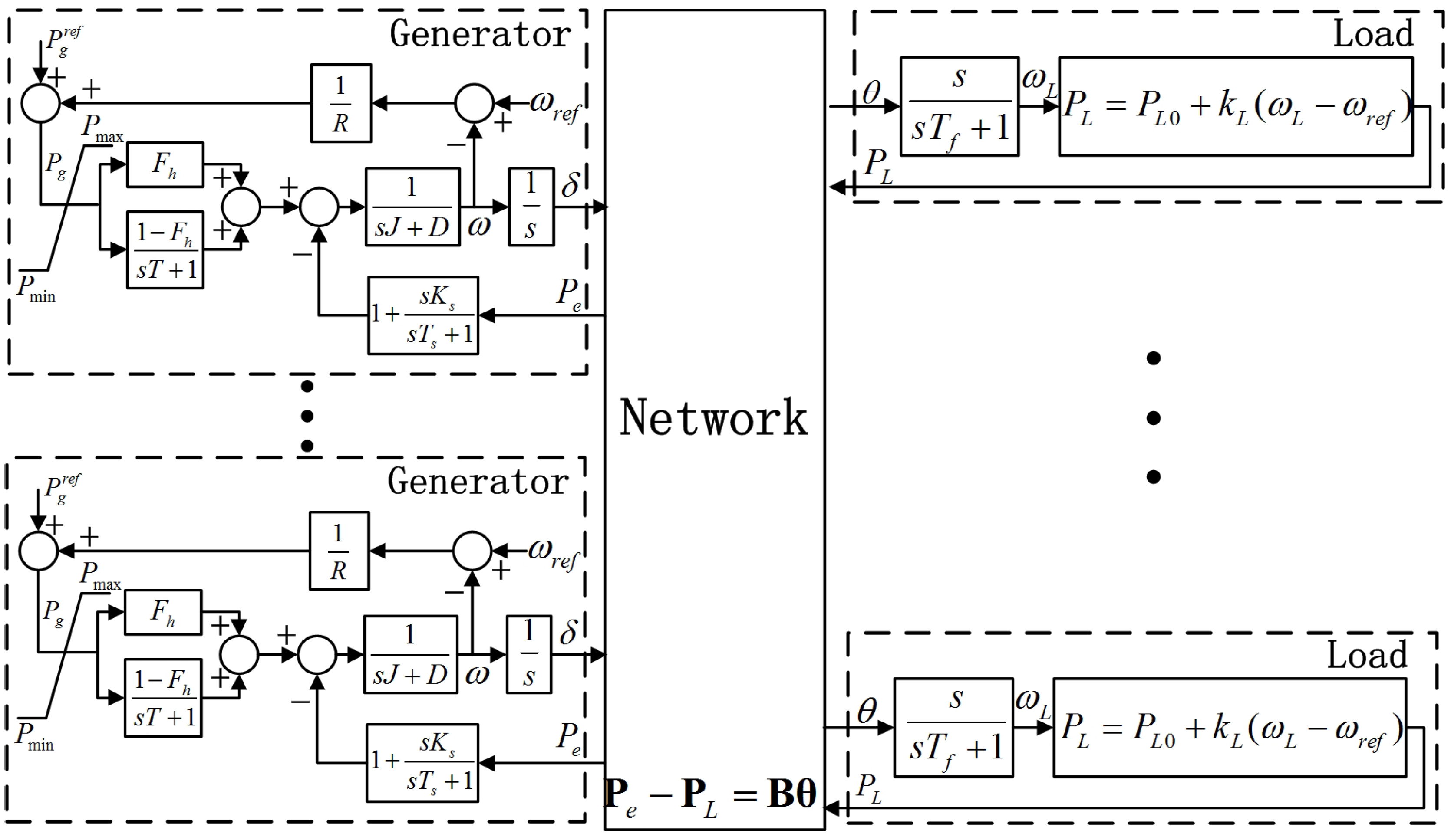
As shown in Figure 3, the whole model consists of three main modules, that is, the individual generator model, electrical load model, and DC power-flow-balance equations of the entire grid.
Firstly, the generator model considers the primary frequency regulator as shown in Equation (1), where the turbine model and rotor motion model are discussed in detail in [6].
where for generator i in generator set , is the mechanical power under primary frequency regulation, whose reference value is . is the value of rated frequency that usually is set as 1.0 p.u., and is the actual frequency value of generator i. and are the difference coefficients of the primary frequency regulator and the total rated capacity, respectively.
Secondly, the frequency-dependent electrical load model is presented in Equation (2), where for load i belonging to load set , is its actual active load, is the rated load value, is its frequency, and is the frequency-dependent coefficient:
Finally, the equation of the power flow distribution across the whole grid is given in Equation (3), where is the vector of nodal generation injection, is the vector of nodal load injection and is the admittance matrix of the grid. Nodal phrase angle vector is denoted as :
In order to combine the aforementioned three parts, two approximations are made as follows: (1) For the purpose of simplicity, the phrase angle of the generator’s terminal bus can be seen the same as the internal phrase angle of the generator. Based on this, the electromagnetic power of the generator can be injected into the power grid directly through the terminal bus; (2) frequency of load can be calculated by first-order differential of phrase angle of the corresponding bus.
It is notable that neglecting the electromagnetic features of the generator may reduce the stability level and cause power fluctuation, which will be validated in Section 3. Thus, a damping block is added to filter the electromagnetic power , just as shown in Figure 3. Its parameters can be optimized by some computational intelligent algorithms [17] to better approach the full-time simulation results.
2.2. Simulation Model of Protection Devices and Supervisory Control Scheme
A variety of advanced protection devices and automatic control systems are installed in the power system to enhance its stability and economy. Obviously, their influence increases the complexity of its dynamic behavior. This makes it rather difficult for researchers to build an ideal simulation model including all factors. Therefore, some important mechanisms that propagate the cascading failures or cause serious loss directly are considered in this paper, including OPB (lines and transformers), AFPG, under-frequency load shedding (UFLS), over-frequency generator tripping (OFGT) and emergency dispatch (ED) by the operators.
2.2.1. Overloading Protection of Branches
Tripping of the overloading branch is one of the most common factors to propagate the cascading process. A simplified accumulative function from [18,19] is used here to measure the overloading severity as shown in Equation (4).
where each branch i belongs to the branch set . Its active power at time t and thermal capacity are denoted as and , respectively. When exceeds , will start to accumulate, indicating the temperature rise due to overloading. Once exceeds a threshold value , branch i should be tripped off by the protection device. It is notable that is not the exact value of heat accumulation on branch i in real situations, but just an indicator of overloading severity. However, it can make a good approximation of the actual characteristics of overloading protections with appropriate value regulation of and .
2.2.2. Abnormal Frequency Protection of Generators
Generators may be damaged when working with too-high or too-low frequency. Abnormal frequency protection can guarantee the continual working of the generator if its measured frequency (or rotor speed) stays in a specific secure range. If frequency falls into an insecure range, the generator will be tripped off within a pre-set time delay. Thus, the frequency dynamics may lead to unwanted tripping of generators in case of severe frequency violation. Table 1 gives some of its typical parameters.
2.2.3. Under-Frequency Load Shedding
UFLS is the last automatic defense to prevent system collapse. The purpose of UFLS is to rebalance generation and load when a significant drop of system frequency occurs. Obviously, UFLS operation will cause load-loss directly, and it is necessary to consider its influence in the proposed model. Operation processes of UFLS are usually divided into several rounds. The parameters of a simplified 4-round UFLS scheme are given in Table 2. It is noted that the UFLS scheme adopted in this paper belongs to the conventional one. As shown in [20,21], sophisticated UFLS schemes make full use of the frequency derivative recorded in local devices or in wide area measurement system (WAMS) to adaptively determine the amount and location of load shedding. This novel kind of UFLS shows good performance, and further studies are needed in the future to reveal its impacts on the cascading failure risk.
2.2.4. Active Over-Frequency Generator Tripping
System frequency will increase if generation capacity surplus exists. Once the frequency exceeds the security threshold, emergency measures should be taken to reduce the output of generators. If system frequency goes back into a secure range again before operations of AFPG, the system will be able to keep frequency security. In practice, direct tripping of generators from the power grid is utilized more commonly than adjusting their output due to the lengthy adjusting time. Thus, a simplified approach is proposed to simulate the OFGT as follows.
If the duration time of the over-frequency state exceeds 5 s, the generator with smallest capacity will be tripped. This process will keep on until system frequency becomes secure or there is left only one generator connected to the grid. This approach approximates the operation in reality.
2.2.5. Emergency Dispatch
ED by operators aims to end the cascading process with the least amount of load shedding, but it may take a long time to complete the calculation and operation. Thus, an assumption is made here to model the real situation: Only when the timespan from the present moment to the nearest future tripping event is long enough, for example, exceeding two min, is it possible for the operation center to complete the ED correctly to terminate the cascading process.
Equations (5)–(10) show a linear programming that determines the optimal load-shedding scheme of ED.
where is the amount shed on load i, and constraints presented in Equations (6)–(10) indicate the power balance equation, the branch flow distribution, power flow limitation of branches, output limitation of generators and load-shedding limitation, respectively.
2.3. Calculation Framework
A differential-algebraic equation (DAE)-based model can be constructed based on the integration of the aforementioned dynamic models and the protection mechanisms. It is shown as follows.
where f and g are linear functions. The state variables , algebraic variables , control variables and discrete variables are introduced here to describe the operational behavior of the protection devices.
The implicit trapezoid method with fixed time-step, usually used in power grid transient analysis, is also utilized here to calculate the numerical solution. Correspondingly, the discretization of Equation (11) is denoted as follows.
Once the values of and at time step k in the iteration process are obtained, the state will be checked for each protection device. For a specific protection device i, whose behavior is represented by , if it has been triggered and the time delay is met at the present time step k, then is set to be 1, indicating that this protection device will disconnect the protected element at time step . Thus, a novel numerical calculation and state-checking-based algorithm is proposed to simulate the cascading failure process. The master routine is demonstrated in Algorithm 1.
| Algorithm 1: Pseudocode of Cascading Failure Simulator |
 |
Specifically, a subroutine is proposed to calculate the numerical solution of each subgrid that is generated after system splitting, and the flow chart is shown in Figure 4. State data of the subgrid at the present time-step k are obtained from the master routine. State checking is then performed for each protection device. If system splitting occurs after operations of some protection devices, the program will jump out of the subroutine. Then, the newly generated subgrids, denoted as , , , , are reserved into buffer . Otherwise, the subroutine will keep on iterating until the cascading process of this subgrid terminates.
For each round of scanning calculations for subgrids reserved in buffer , the newly generated subgrids will be reserved into buffer . After the new assignment from to , the iteration keeps carrying on until no subgrids are generated. Finally, the statistics of load loss and element loss are obtained.
2.4. Model Validation
Simulation is performed on the IEEE 39-bus benchmark to validate the proposed model against a full-time transient model. As a comparison, simulations are made with these two models. In full-time transient simulation, the Type I excitation model and Type I turbine model are considered, whose parameters can be obtained according to the typical values in PSAT software [22]. Parameters of modules in the proposed model are set to be the same as the corresponding ones in the full-time transient model, including parameters of turbine governor, inertia constant and rotor-damping coefficient.
The total timespan of simulation is 50 s. The initial N-2 outages of branches 16–21 and 23–24 occur at time s. The whole system splits into two parts after initial outages. Power-flow changes on branches 2–3 and 2–25, and frequency and output changes of generators at Bus 31 and 35 are demonstrated in Figure 5. It can be observed that with or without the additional damping block, the DFR model can approach the full-time transient model with a high degree of accuracy in terms of generator output. However, there are obvious oscillations in branch power flow and generator frequency obtained by the DFR model without the additional damping module. This shows the fact that neglecting the electromagnetic features of the generator will reduce the systemic damping and cause oscillation. Moreover, it is shown that the additional damping block proposed in this paper can help to improve the accuracy of the DFR model without changing its static regulation characteristics. It takes 112.79 s to complete the calculation with the full-time transient simulation, but only 3.77 s with the proposed model. Therefore, the proposed model in this paper has much higher computational efficiency.
Another concern is the influence of error caused by transmission loss. This is the inherent discrepancy between DC flow-based models and alternating current (AC) flow-based models. However, for the large-scale power grid with high voltage level, the reactance of a branch is much larger than its resistance, and this error usually does not exceed 5%, which is acceptable for general system analysis.
3. Case Studies
3.1. Simulation Setup
Case studies were made in the IEEE 39-bus system, whose data sets are from Matpower 4.1 [23]. The IEEE 39-bus system has 39 nodes, 46 branches and 10 generators. Its total load capacity and maximum generation capacity are 62.54 p.u. and 70.0 p.u., respectively. The threshold values for the accumulative functions are set to guarantee that overloading branches will be tripped off in 20 s when carrying 150% rated capacity. Parameters of abnormal frequency protection and UFLS can be determined just as shown in Table 1 and Table 2, respectively. The timespan for operators to make ED is set as two minutes, so that if the timespan from the present moment to the nearest future tripping event exceeds two minutes, operators have enough time to redispatch the generation profile to terminate the cascading process.
3.2. Case Studies on IEEE 39-Bus System
3.2.1. Demonstration of Dynamic Process
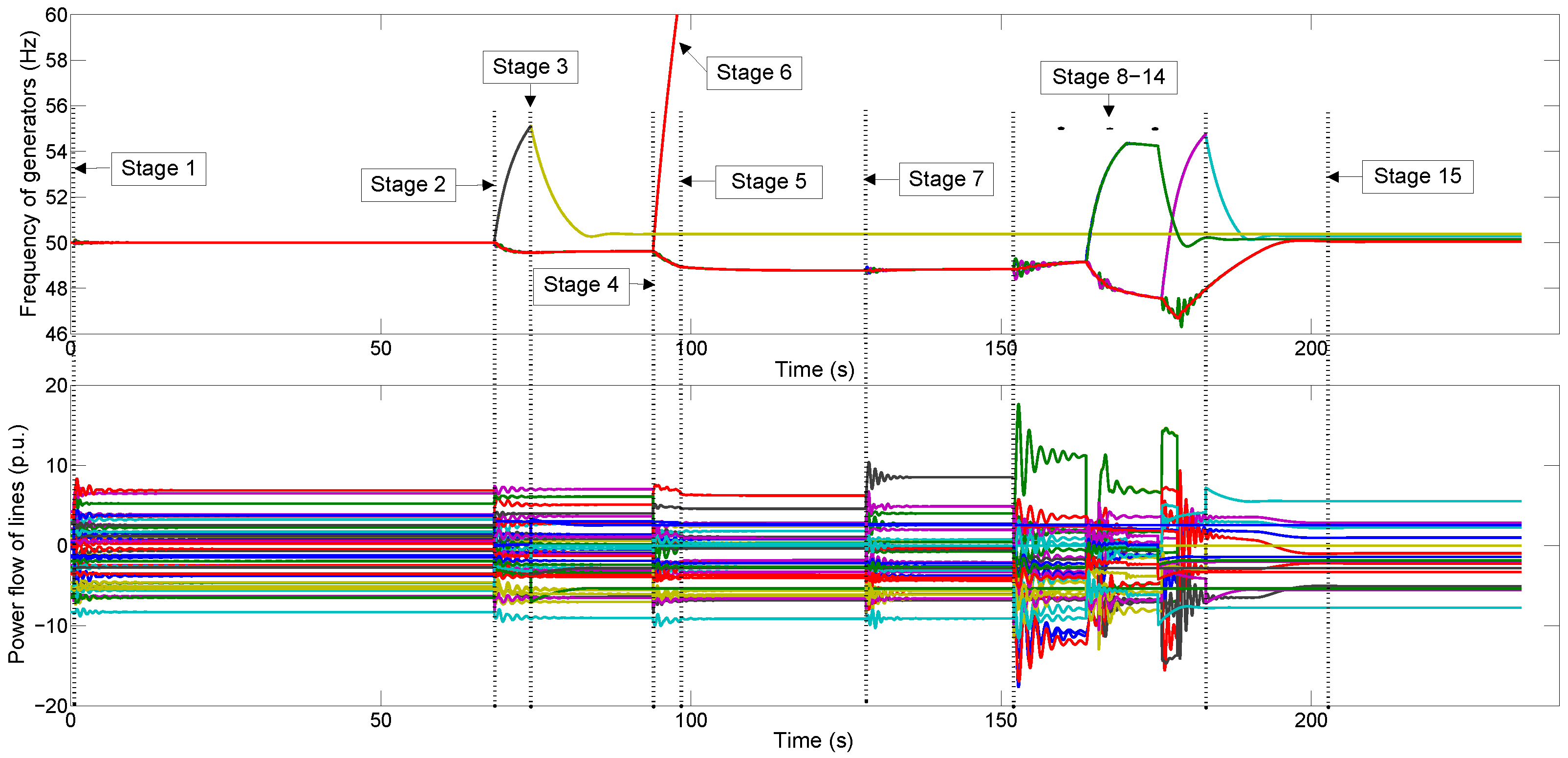
The structure diagram of the IEEE 39-bus system is shown in Figure 6. The initial outages are triggered on branches 10–11 and 16–21 to start the dynamic process. The detailed list of cascading events in the dynamic process is shown in Table 3, and the curves of generator frequency and power flow on branches are shown in Figure 7.
The dynamic process can be elaborated as follows. After initial outages of branches 10–11 and 16–21 at t = 0.5 s, branches 23–24 and 10–13 became overloaded.Since the time was not long enough for operators to eliminate the overloading, both branches were tripped by overloading protection at t = 68.4 s and t = 93.9 s, respectively. Then, the whole system broke into three subgrids, that is, one consisting of buses 10 and 32, one consisting of buses 21–23, 35 and 36, and one consisting of the other buses. Different frequency dynamics emerged in these subgrids. The frequency of the generator at bus 32 increased rather rapidly since there was no load in this subgrid. It was finally tripped by over-frequency protection at time t = 124.6 s. A similar situation appeared in the subgrid including buses 21–23, 35 and 36. However, the generator at bus 36 was disconnected by active over-frequency tripping at time t = 74.2 s, and then the frequency of this subgrid remained secure. No further events occurred in this subgrid. On the opposite side, the frequency of the third subgrid dropped down due to the generation shortage. This triggered the first round of UFLS, which shed 5% load sequentially between s and s. Some further cascading events occurred afterwards in the cascading process, such as branch outages, UFLS operation and generator outages.
As shown in Figure 6, the whole grid split into six parts finally, which were labelled as I, II, III, IV, V and VI. Subgrids I, III, IV and V retained frequency security, but subgrid II did not. Subgrid VI collapsed due to the complete loss of power supply. The total load loss is 28.22 p.u. Some observations can be made from this simulation:
- Frequency dynamics and power-flow transfer are closely coupled to affect the dynamic process. Frequency-related protections may cause serious load shedding or infrastructure failures.
- Time intervals between adjacent events become shorter as the cascading process propagates. As shown in Figure 7, the system undergoes fast state changes from Stage 8 to Stage 14. In this period, many protection devices are triggered intensively. Thus, ED is not available once the system comes into this period.
- Load loss may be induced by several factors, for example, UFLS, subgrid collapse due to generator outages, losing power supply due to branch outages, ED, and so on. Statistics show that the frequency insecurity-induced load loss, which is caused by the first two factors aforementioned, is 15.52 p.u., accounting for about 55% of total load loss. Moreover, five generators were tripped by abnormal frequency protection. It can be seen that frequency insecurity has great impacts on the safety of the power grid, especially when power mismatch emerges after unplanned system splitting.
3.2.2. Statistical Results
In order to further reveal the impact of frequency insecurity, exhaustive screening for all N-2 initial branch outages is made to obtain the samples. For each specific simulation, the frequency insecurity-induced load loss is referred to as those with the following two features:
- shed by UFLS operation directly;
- in subgrid that collapsed due to generator tripping under abnormal frequency.
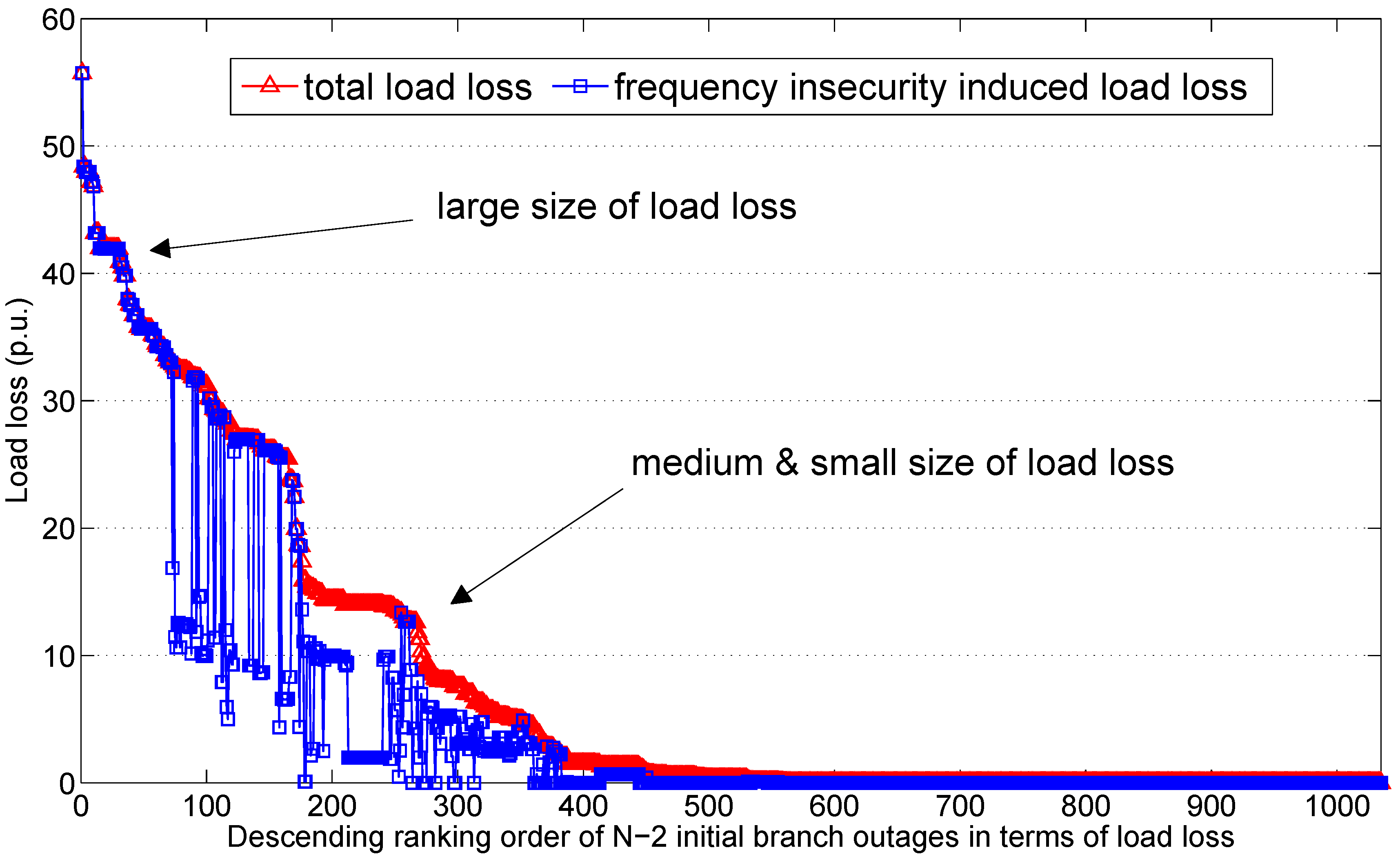
There are N-2 branch outages. The red curve with triangular marks in Figure 8 represents the descending ranking of N-2 branch outages in terms of size of load loss. Meanwhile, the corresponding frequency insecurity-induced load loss is depicted by the blue curve with rectangular marks. From Figure 8, it is interesting to see that the initial outages resulting in large total load loss tend to have extremely high proportions of frequency insecurity-induced load loss in general. However, for those leading to medium and small sizes of total load loss, the proportion of frequency insecurity-induced load loss is relatively lower. The frequency insecurity becomes a more dominant factor when load loss of the power blackout increases. These results demonstrate the threat of frequency insecurity to the power system.
Monte Carlo simulation is also introduced to demonstrate this influence quantitatively. Assuming that the probability of being tripped initially for each branch is p, then N times of random experiments are carried out under each given p. An index is proposed to quantify the average ratio of frequency insecurity-induced load loss to the total load loss as follows.
where is the label set of simulation samples with nonzero load loss. and are frequency insecurity-induced load loss and total load loss of the ith experiment, respectively. N is set to be 5000, the value of p increases from 0.01 to 0.1 with the step of 0.01.
As shown in Figure 9, as the value of p increases from 0.01 to 0.1, average total load loss (p.u.) increases sharply from 1.17 p.u. to 20.79 p.u. Meanwhile, the corresponding value of also increases from 0.37 to 0.67. It means that as p increases, the power system will be exposed to a situation with greater risk of load loss, and the frequency insecurity-induced load loss will also account for a higher and higher proportion. The increment of load loss is largely due to the worsening of frequency security. Obviously, this is another point indicating the strong threat of frequency insecurity to the power system. Integrating the aforementioned discussion, we can conclude that it is suggested to improve the frequency-regulation performance to enhance the robustness of a power system against disturbance.
3.2.3. Influence of Spinning Reserve Capacity
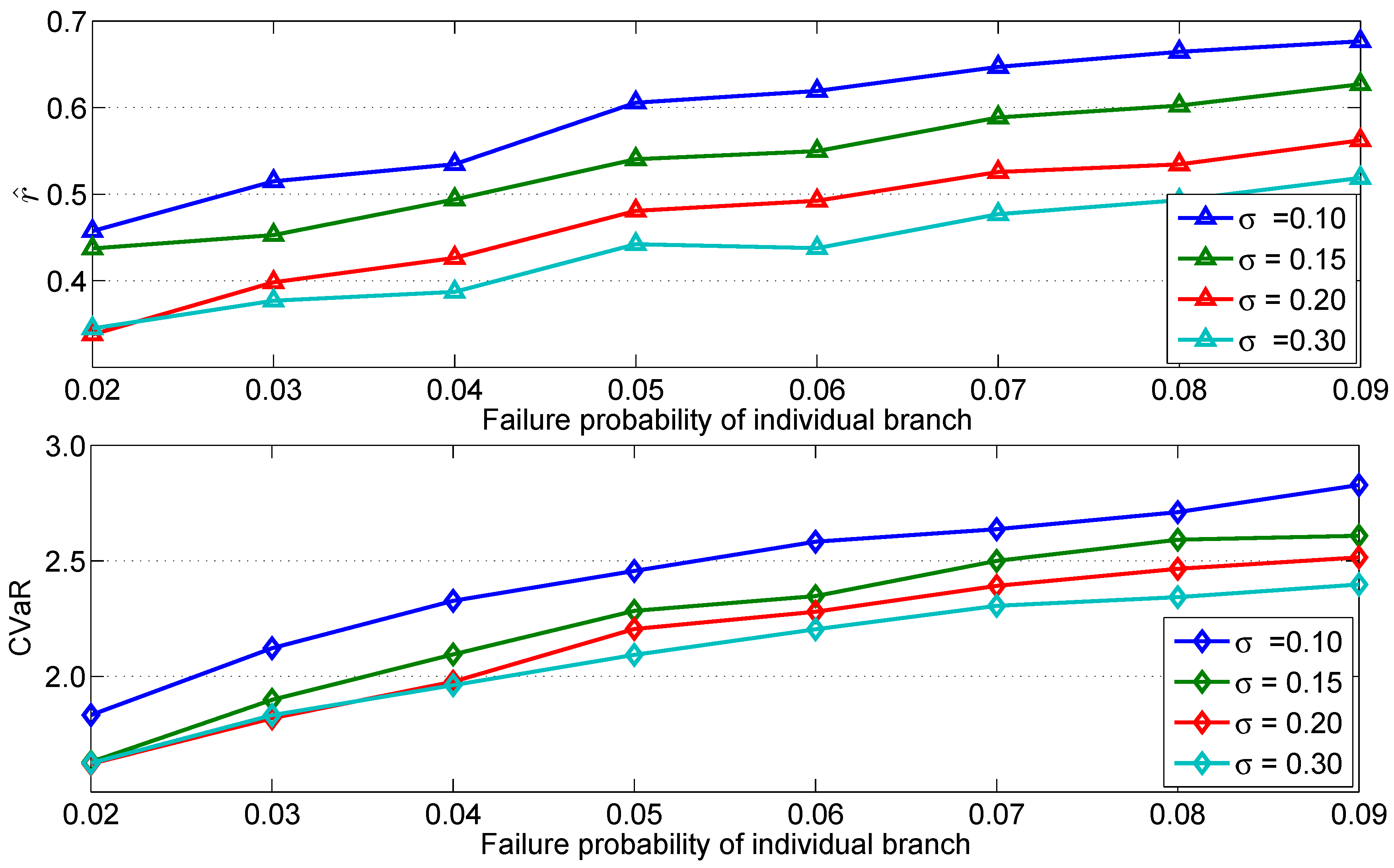
Usually, a generator that participates in primary frequency regulation has a certain boundary to limit its output. This boundary determines its spinning reserve capacity. The spinning reserve capacity also has a great influence on the frequency-regulation performance. For generator i, its output range can be expressed by , where is a ratio whose value is usually between 10% and 20%. This paper assesses system security under different reserve capacities by changing from 10% to 30%. Due to the fat-tail characteristics shown in Figure 8, the conditional value-at-risk (CVaR) is used to evaluate the risk level of a power system when suffering large-scale load loss just as shown in Equation (14), where is the confidence probability [9]. and satisfies that .
Letting be 95%, values of and under different and p are depicted in Figure 10. Some useful observations can be obtained as follows:
- increases rapidly as the failure probability p increases; meanwhile, adequate spinning reserve capacity dramatically reduces this risk.
- In general, as the ratio of spinning reserve capacity increases, the proportion of frequency insecurity-induced load loss reduces dramatically.
- Especially when the initial disturbance is less threatening, such as when , the marginal utility of increasing reserve capacity becomes weaker as continues to increase. Thus, increasing the reserve capacity is more effective when the external disturbance tends to be more serious.
4. Conclusions and Discussion
In this paper, we explore the detailed process of a real power blackout, acquiring the fact that maintaining frequency security during the blackout is vital for the power system. Then, a comprehensive simulation model considering frequency dynamics and possible cascading events is proposed. Protection devices and supervisor control schemes are taken into account by this model. Statistical results of case studies demonstrate the important role of frequency insecurity in causing power blackout from the viewpoint of simulation. Hence, it is worth improving the frequency-regulation performance in case of emergency to cope with the challenges of a power blackout.
However, work in this paper should be just seen as the basis of further revealing the frequency security-related features in a power blackout. In future work, stochastic behavior of frequency-related protection devices can be introduced in this model to evaluate the security risk of systems more comprehensively. With this model, the influence of different advanced frequency-control schemes on the power blackout can be revealed, for example, decentralized UFLS, and WAMS-based centralized UFLS. Moreover, the method of optimally allocating the spinning reserve capacity to enhance the security of the power system will also be studied.
Acknowledgments
This work is supported by the National Natural Science Foundation of China (51190105, 51277135) and the State Grid Technology Project of China (XT71-12-011).
Author Contributions
Chao Luo, Jun Yang and Yuanzhang Sun conceived and designed the experiments; Chao Luo performed the experiments; Chao Luo analyzed the data; Jun Yang and Yuanzhang Sun contributed reagents/materials/analysis tools; Chao Luo wrote the paper.
Conflicts of Interest
The authors declare no conflict of interest. The founding sponsors had no role in the design of the study; in the collection, analyses, or interpretation of data; in the writing of the manuscript, and in the decision to publish the results.
References
- Andersson, G.; Donalek, P.; Farmer, R.; Hatziargyriou, N.; Kamwa, I.; Kundur, P.; Martins, N.; Paserba, J.; Pourbeik, P.; Sanchez-Gasca, J.; et al. Causes of the 2003 major grid blackouts in North America and Europe, and recommended means to improve system dynamic performance. IEEE Trans. Power Syst. 2005, 20, 1922–1928. [Google Scholar] [CrossRef]
- Enquiry Committee. Report of the Enquiry Committee on Grid Disturbance in Northern Region on 30 July 2012 and in Northern, Eastern & North-Eastern Region on 31 July 2012. Available online: http://www.powermin.nic.333in\/pdf\/GRID_ENQ_REP_16_8_12.pdf (accessed on 25 January 2018).
- Maas, G.; Bial, M.; Fijalkowski, J. Final Report-System Disturbance on 4 November 2006; Technical Report; Union for the Coordination of Transmission of Electricity in Europe: Brussels, Belgium, 4 November 2007. [Google Scholar]
- Kunitomi, K.; Kurita, A.; Tada, Y.; Ihara, S.; Price, W.; Richardson, L.; Smith, G. Modeling combined-cycle power plant for simulation of frequency excursions. IEEE Trans. Power Syst. 2003, 18, 724–729. [Google Scholar] [CrossRef]
- Lin, W.; Sun, H.; Tang, Y.; Bu, G.; Yin, Y. Analysis and lessons of the blackout in Brazil power grid on November 10, 2009. Autom. Electr. Power Syst. 2010, 1676, 43–50. [Google Scholar]
- Anderson, P.M.; Mirheydar, M. A low-order system frequency response model. IEEE Trans. Power Syst. 1990, 5, 720–729. [Google Scholar] [CrossRef]
- Chan, M.L.; Dunlop, R.; Schweppe, F. Dynamic equivalents for average system frequency behavior following major distribances. IEEE Trans. Power Appar. Syst. 1972, PAS-91, 1637–1642. [Google Scholar] [CrossRef]
- Qi, J.; Mei, S.; Liu, F. Blackout model considering slow process. IEEE Trans. Power Syst. 2013, 28, 3274–3282. [Google Scholar] [CrossRef]
- Mei, S.; He, F.; Zhang, X.; Wu, S.; Wang, G. An improved OPA model and blackout risk assessment. IEEE Trans. Power Syst. 2009, 24, 814–823. [Google Scholar]
- Yu, Y.; Gan, D.; Wu, H.; Han, Z. Frequency induced risk assessment for a power system accounting uncertainties in operation of protective equipments. Int. J. Electr. Power Energy Syst. 2010, 32, 688–696. [Google Scholar] [CrossRef]
- Ren, H.; Dobson, I.; Carreras, B.A. Long-term effect of the n-1 criterion on cascading line outages in an evolving power transmission grid. IEEE Trans. Power Syst. 2008, 23, 1217–1225. [Google Scholar] [CrossRef]
- Nedic, D.P.; Dobson, I.; Kirschen, D.S.; Carreras, B.A.; Lynch, V.E. Criticality in a cascading failure blackout model. Int. J. Electr. Power Energy Syst. 2006, 28, 627–633. [Google Scholar] [CrossRef]
- Wang, Y.; Baldick, R. Interdiction Analysis of Electric Grids Combining Cascading Outage and Medium-Term Impacts. IEEE Trans. Power Syst. 2014, 29, 2160–2168. [Google Scholar] [CrossRef]
- Tu, J.; Xin, H.; Wang, Z.; Gan, D.; Huang, Z. On Self-Organized Criticality of the East China AC–DC Power System—The Role of DC Transmission. IEEE Trans. Power Syst. 2013, 28, 3204–3214. [Google Scholar] [CrossRef]
- Song, J.; Cotilla-Sanchez, E.; Ghanavati, G.; Hines, P.D. Dynamic Modeling of Cascading Failure in Power Systems. arXiv, 2014; arXiv:1411.3990. [Google Scholar]
- Li, C.; Liu, Y.; Zhang, H. Fast analysis of active power-frequency dynamics considering network influence. In Proceedings of the 2012 IEEE Power and Energy Society General Meeting, San Diego, CA, USA, 22–26 July 2012; pp. 1–6. [Google Scholar]
- Tang, Y.; Ju, P.; He, H.; Qin, C.; Wu, F. Optimized Control of DFIG-Based Wind Generation Using Sensitivity Analysis and Particle Swarm Optimization. IEEE Trans. Smart Grid 2013, 4, 509–520. [Google Scholar] [CrossRef]
- Eppstein, M.J.; Hines, P.D. A “Random Chemistry” algorithm for identifying collections of multiple contingencies that initiate cascading failure. IEEE Trans. Power Syst. 2012, 27, 1698–1705. [Google Scholar] [CrossRef]
- Yan, J.; Tang, Y.; He, H.; Sun, Y. Cascading Failure Analysis With DC Power Flow Model and Transient Stability Analysis. IEEE Trans. Power Syst. 2014, 30, 285–297. [Google Scholar] [CrossRef]
- Rudez, U.; Mihalic, R. WAMS-Based Underfrequency Load Shedding With Short-Term Frequency Prediction. IEEE Trans. Power Deliv. 2016, 31, 1912–1920. [Google Scholar] [CrossRef]
- Rudez, U.; Mihalic, R. Monitoring the First Frequency Derivative to Improve Adaptive Underfrequency Load-Shedding Schemes. IEEE Trans. Power Syst. 2011, 26, 839–846. [Google Scholar] [CrossRef]
- Milano, F.; Vanfretti, L.; Morataya, J.C. An open source power system virtual laboratory: The PSAT case and experience. IEEE Trans. Educ. 2008, 51, 17–23. [Google Scholar] [CrossRef]
- Zimmerman, R.D.; Murillo-Sánchez, C.E.; Thomas, R.J. MATPOWER: Steady-state operations, planning, and analysis tools for power systems research and education. IEEE Trans. Power Syst. 2011, 26, 12–19. [Google Scholar] [CrossRef]
Figure 1.
(a) Schematic map of UCTE area that split into three areas; and (b) frequency recordings after the split in the blackout on 4 November 2006, in the European interconnected electric grid [3].
Figure 1.
(a) Schematic map of UCTE area that split into three areas; and (b) frequency recordings after the split in the blackout on 4 November 2006, in the European interconnected electric grid [3].

Figure 2.
Block diagram of (a) system frequency response (SFR) model; and (b) average system frequency (ASF) model.
Figure 2.
Block diagram of (a) system frequency response (SFR) model; and (b) average system frequency (ASF) model.
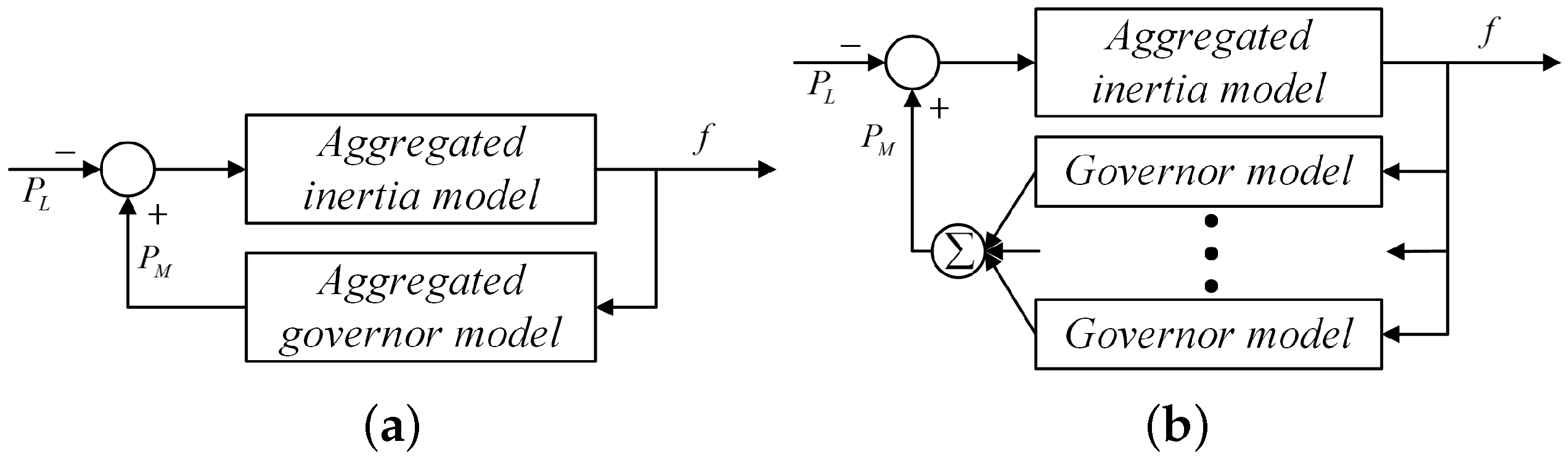
Figure 3.
Diagram of DFR model.

Figure 4.
Flow chart of island calculation subroutine.
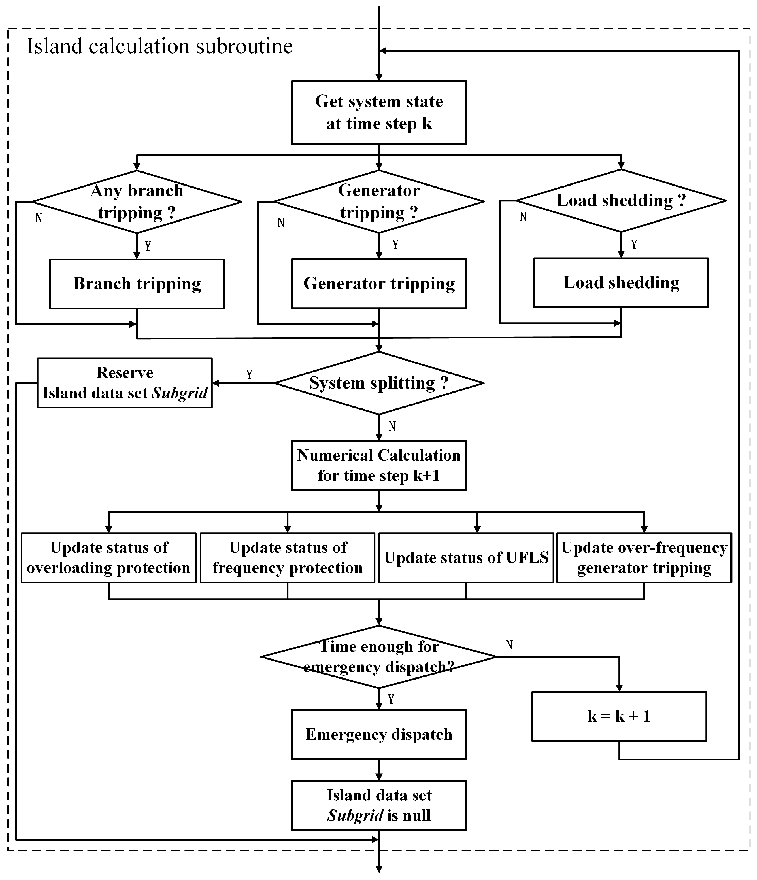
Figure 5.
Dynamics of generator output, frequency and branch power flow after initial outages of branch 16–21 and branch 23–24 at s in the IEEE 39-bus system.
Figure 5.
Dynamics of generator output, frequency and branch power flow after initial outages of branch 16–21 and branch 23–24 at s in the IEEE 39-bus system.
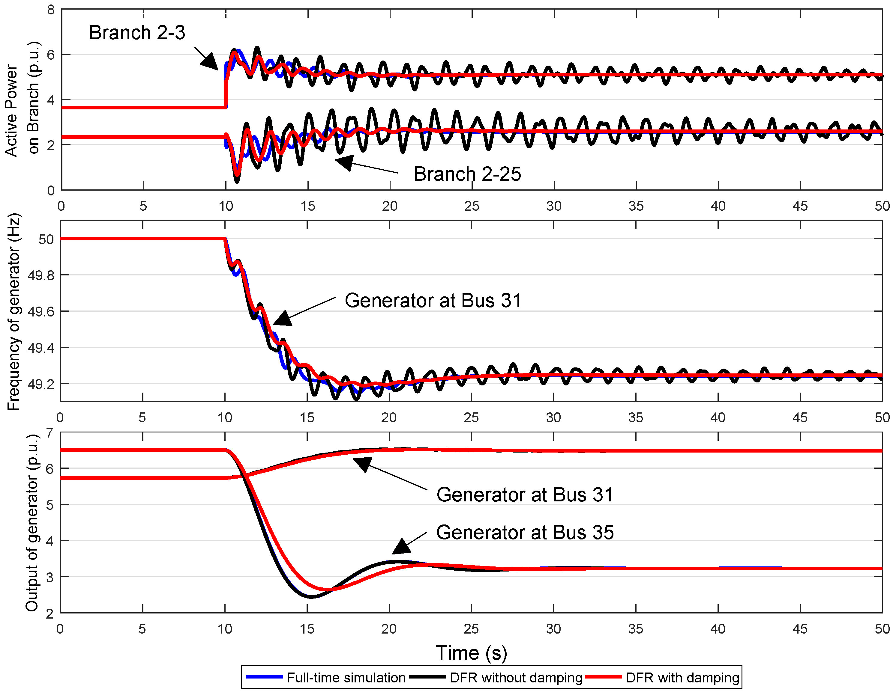
Figure 6.
Structure diagram of IEEE 39-bus test system. The split regions marked by red dashed lines will be later discussed in Section 3.
Figure 6.
Structure diagram of IEEE 39-bus test system. The split regions marked by red dashed lines will be later discussed in Section 3.
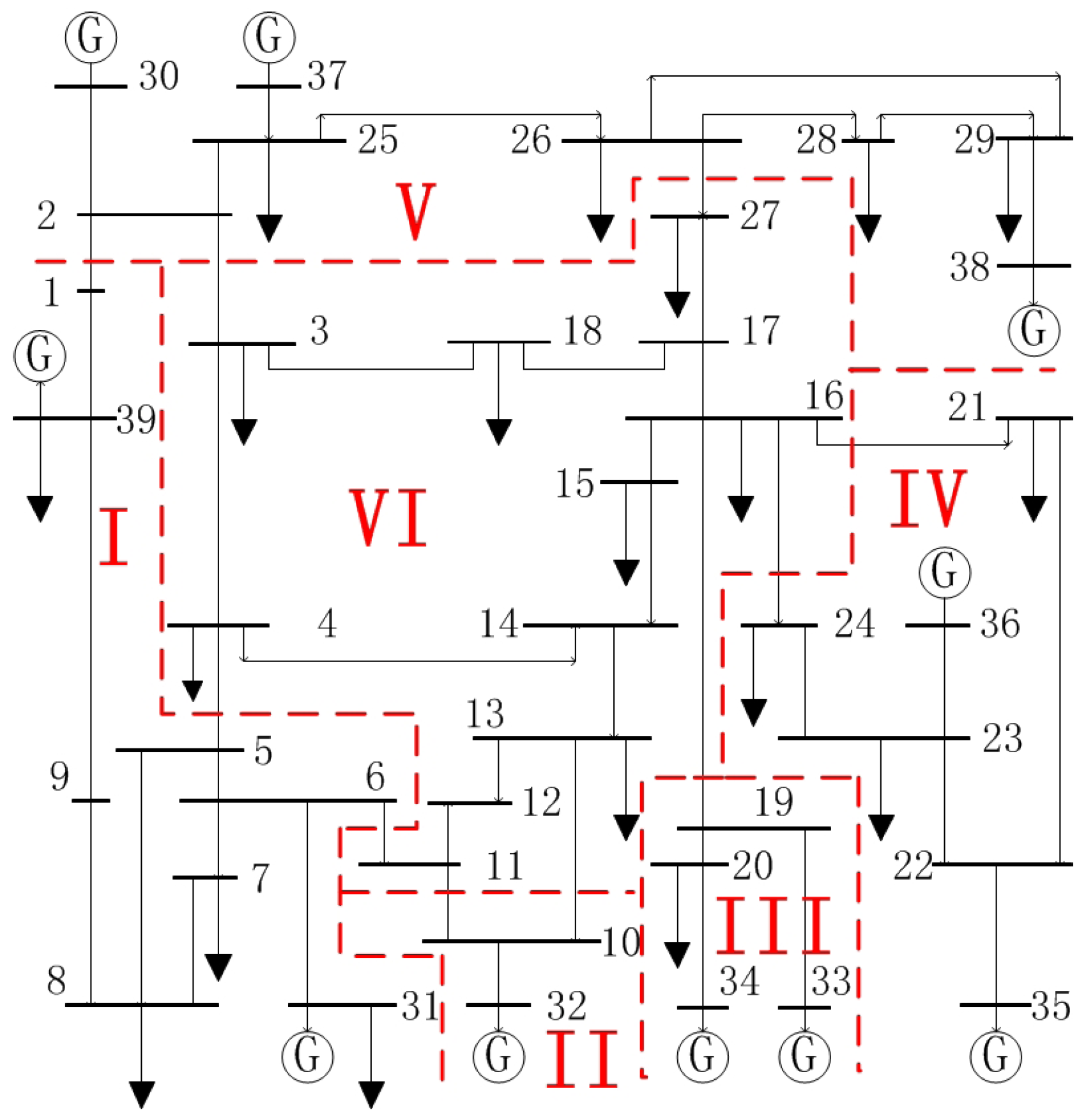
Figure 7.
Dynamics of generator frequency and branch power flow after initial outages of branches 10–11 and 16–21.
Figure 7.
Dynamics of generator frequency and branch power flow after initial outages of branches 10–11 and 16–21.

Figure 8.
Statistics of load loss under N-2 initial branch outages in the IEEE 39-bus system.

Figure 9.
Average ratio of frequency insecurity-induced load loss to the total load loss under different p.
Figure 9.
Average ratio of frequency insecurity-induced load loss to the total load loss under different p.
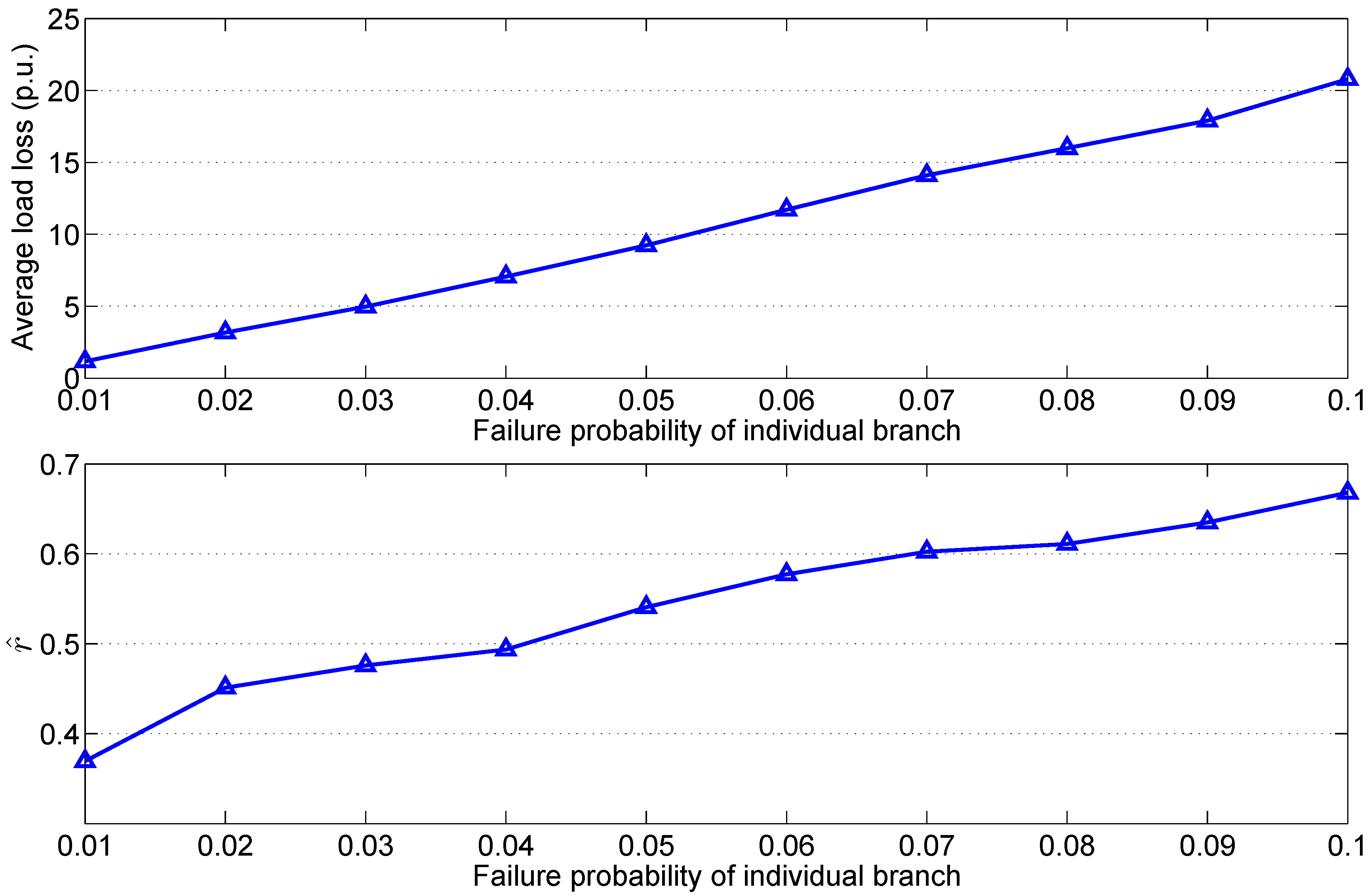
Figure 10.
Average ratio of frequency insecurity-induced load loss to the total load loss and the conditional value-at-risk (CVaR) under different p and .
Figure 10.
Average ratio of frequency insecurity-induced load loss to the total load loss and the conditional value-at-risk (CVaR) under different p and .


Table 1.
Parameters of abnormal frequency protection.
| Num. | Frequency Range | Time Delay |
|---|---|---|
| 1 | <47.0 Hz | 10 s |
| 2 | 47.0 Hz–48.5 Hz | 40 s |
| 3 | 48.5 Hz–51.0 Hz | continual working |
| 4 | 51.0 Hz–52.0 Hz | 60 s |
| 5 | >52.0 Hz | 30 s |
Table 2.
Parameters of under-frequency load shedding (UFLS).
| Round | Trigger Frequency | Ratio of Load Shedding | Time Delay |
|---|---|---|---|
| 1 | 49.00 Hz | 5% | 0.5 s |
| 2 | 48.75 Hz | 5% | 0.5 s |
| 3 | 48.50 Hz | 5% | 0.5 s |
| 4 | 48.25 Hz | 5% | 0.5 s |
Table 3.
Event list of cascading process.
| Stage | Events | Time Moment |
|---|---|---|
| 1 | IBranch 10–11 and Branch 16–21 outages | t = 0.5 s |
| 2 | Branch 23–24 outage | t = 68.3 s |
| 3 | Generator at Bus 36 outage | t = 74.2 s |
| 4 | Branch 10–13 outage | t = 93.9 s |
| 5 | UFLS at Bus 3, 4, 7, 8, 12, 15, 16, 18, 20, 24–29, 31, 39 (1st round) | t = 98.1–98.4 s |
| 6 | Generator at Bus 32 outage | t = 124.6 s |
| 7 | Branch 2–3 outage | t = 128.2 s |
| 8 | Branch 26–27 outage | t = 152.0 s |
| 9 | UFLS at Bus 3, 4, 7, 8, 12, 15, 16, 18 20,24–29, 31, 39 (2nd round) | t = 152.5 s–165.2 s |
| 10 | Branch 1–2 outage | t = 163.7 s |
| 11 | Branch 4–5 outage | t = 165.7 s |
| 12 | UFLS at Bus 3, 4, 7, 8, 12, 15, 16, 18 20, 24, 27, 31, 39 (3rd round) | t = 165.9 s–166.5 s |
| 13 | UFLS at Bus 3, 4, 7, 8, 12, 15, 16, 18 20, 24, 27, 31, 39 (4th round) | t = 166.5 s–167.3 s |
| 14 | Generator at Bus 30 outage | t = 170.2 s |
| 14 | Generator at Bus 37 outage | t = 175.3 s |
| 15 | Branch 16–19 outage | t = 175.9 s |
| 16 | Branch 6–11 outage | t = 178.4 s |
| 14 | Generator at Bus 34 outage | t = 183.0 s |
| 15 | Emergency Dispatch (ED) | t = 205.1 s–228.8 s |
© 2018 by the authors. Licensee MDPI, Basel, Switzerland. This article is an open access article distributed under the terms and conditions of the Creative Commons Attribution (CC BY) license (http://creativecommons.org/licenses/by/4.0/).
Share and Cite
MDPI and ACS Style
Luo, C.; Yang, J.; Sun, Y. Risk Assessment of Power System Considering Frequency Dynamics and Cascading Process. Energies 2018, 11, 422. https://doi.org/10.3390/en11020422
AMA Style
Luo C, Yang J, Sun Y. Risk Assessment of Power System Considering Frequency Dynamics and Cascading Process. Energies. 2018; 11(2):422. https://doi.org/10.3390/en11020422
Chicago/Turabian StyleLuo, Chao, Jun Yang, and Yuanzhang Sun. 2018. "Risk Assessment of Power System Considering Frequency Dynamics and Cascading Process" Energies 11, no. 2: 422. https://doi.org/10.3390/en11020422
Note that from the first issue of 2016, this journal uses article numbers instead of page numbers. See further details here.