Article

Derivation and Application of a New Transmission Loss Formula for Power System Economic Dispatch

1
Department of Industrial Education and Technology, National Changhua University of Education, No. 2, Shida Rd., Changhua 500, Taiwan
2
The Institute of Nuclear Energy Research, 1000 Wenhua Rd., Jiaan Village, Longtan Dist., Taoyuan City 325, Taiwan
*
Authors to whom correspondence should be addressed.
Energies 2018, 11(2), 417; https://doi.org/10.3390/en11020417
Submission received: 31 December 2017 / Revised: 29 January 2018 / Accepted: 7 February 2018 / Published: 11 February 2018
(This article belongs to the Section F: Electrical Engineering)

Abstract

:
The expression and calculation of transmission loss (TL) play key roles for solving the power system economic dispatch (ED) problem. ED including TL must compute the total TL and incremental transmission loss (ITL) by executing power flow equations. However, solving the power flow equations is time-consuming and may result in divergence by the iteration procedure. This approach is unsuitable for real-time ED in practical power systems. To avoid solving nonlinear power flow equations, most power companies continue to adopt the TL formula in ED. Traditional loss formulas are composed of network parameters and in terms of the generator’s real power outputs. These formulas are derived by several assumptions, but these basic assumptions sacrifice accuracy. In this study, a new expression for the loss formula is proposed to improve the shortcomings of traditional loss formulas. The coefficients in the new loss formula can be obtained by recording the power losses according to varying real and reactive power outputs without any assumptions. The simultaneous equations of the second-order expansion of the Taylor series are then established. Finally, the corresponding coefficients can be calculated by solving the simultaneous equations. These new coefficients can be used in optimal real and reactive power dispatch problems. The proposed approach is tested by IEEE 14-bus and 30-bus systems, and the results are compared with those obtained from the traditional B coefficient method and the load flow method. The numerical results show that the proposed new loss formula for ED can hold high accuracy for different loading conditions and is very suitable for real-time applications.

1. Introduction

The economic dispatch (ED) problem [1,2,3,4,5] in a modern power system involves allocating the output power of each generator to minimize the total cost of the power generation satisfying load demand and transmission loss (TL) under the constraints of the generators’ limits, line congestion, emission, renewable energy resources, and demand response. In a large interconnected power system, power is transmitted over long distances to distribution systems; consequently, TL is the dominating factor in power system ED. In determining the economic power dispatch to satisfy the load demand between the generators, the total TL of the system can be expressed in terms of the real power output of each generator. The simplified ED in a short transmission distance and high load-density power system can ignore the TL so that the computation model is simple and only uses the equal incremental cost equation [6] to obtain the best allocation. However, this solution is not optimal because TL is ignored. This disregard is due to TL being around 4–8% of the total load. For instance, the line loss of the Taipower system was 4.76% in 2011. This percentage is sufficient to affect the overall cost of allocation. To overcome this problem, related studies focus on deriving TL formulas [7,8,9,10,11] for ED or executing power flow-based ED to include TL in the optimal solution for obtaining an exact solution [12,13,14]. The drawback of including the TL in the power flow equation for solving the optimal ED is that the TL and incremental transmission loss (ITL) need to be re-calculated in each iteration, and this iterative process is very time-consuming and even leads to convergence problems. Solving the ED problem using the loss formula does not present the aforementioned problems. TL can be expressed as a quadratic function of real power generations at each generator bus. The most well-known formula is the quadratic expression of loss, which was proposed by George et al. [9,10]. Another well-known and widely adopted quadratic polynomial equation was developed by Kron and promoted and applied by Kirchmayer [10]. After the loss formulas became more developed, few new works have been done. Only Andrew Jiang [15] proposed general polynomial loss formulas, in which TL can be expressed as a function of real power outputs of generating units in second-order and even higher-order term polynomials. This expression is complicated, and only few scholars have accepted these models. In summary, accurate TL formulas are composed of linear, quadratic, and high-order terms. Regardless of the types of loss models derived, calculating the coefficients by interpolating a small number of power flow solutions is crucial, and the purpose of these loss formulas is to solve ED. In general, two common approaches are used to solve the ED problem; one is the conventional method by nonlinear programming techniques, which can only solve for the convex objective function by gradient or Newton-based search algorithms [6,16]. The other is an artificial intelligence method by metaheuristic techniques for solving convex or nonconvex problems. These algorithms are the genetic algorithm [17,18], the evolutionary algorithm [19], particle swarm optimization [20,21,22], simulated annealing [23], bee colony optimization [24], tabu search [25], the bat algorithm [26], and mixed-integer nonconvex nonlinear programming [27]. These algorithms have been successfully implemented to solve ED problems, whereas the B coefficient method is commonly used to calculate TL in the ED problem of the above works in the power utility industry. Therefore, the loss formula plays a key role for power system ED.
This study proposes a novel method for determining the loss coefficients and a new loss formula model. The proposed method for determining the Kron’s loss coefficients does not need any assumptions. The method only requires power output variations, which are the same times as the unknown coefficients. Each change of TL caused by power output variations should also be recorded. Subsequently, solving these simultaneous equations can yield all unknown coefficients. This paper is divided into five sections. Section 1 introduces the background and objectives of this study. Section 2 describes the problem of the common approaches in power system ED and the derivation procedure of B coefficients of the proposed loss formula. Section 3 details the derivation of new loss formulas and its application to ED. Section 4 discusses the simulation results. Section 5 presents our conclusions.

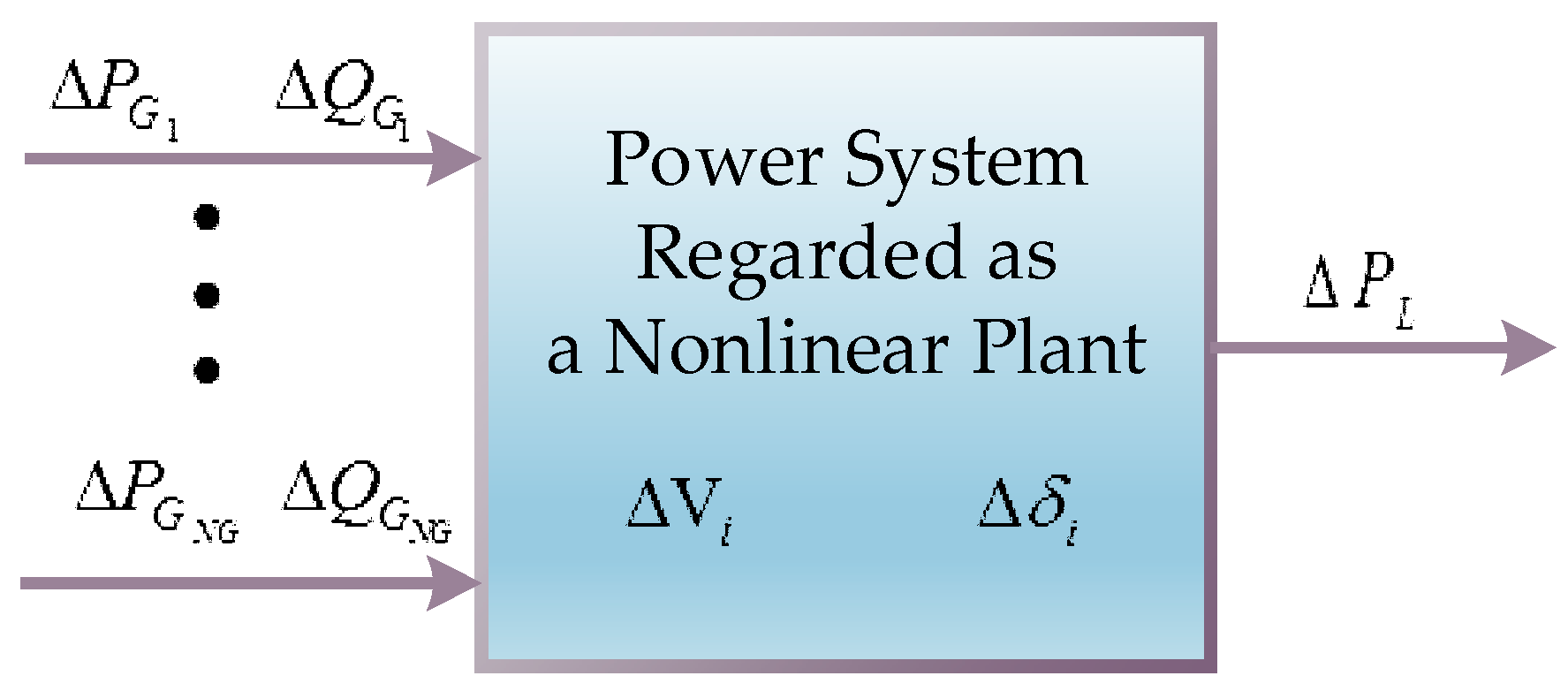
2. Problem Description

The ED problem of a power system must take into account the power balance, including TL and load demand with minimum fuel cost, without violating the limits of generator rating and transmission capacity simultaneously. Especially in a large-scale interconnected power grid, TL is the major factor affecting ED. Two common approaches in ED including TL are power flow-based ED and B coefficient-based ED [6]. The former is time-consuming and has convergence risk; therefore, it is unsuitable for real-time applications. For practical application, B coefficient-based ED should establish more than one set of B coefficients during the daily load cycle because B coefficients are not truly constant as they vary with load demand. The B coefficients can be obtained by the traditional loss coefficient formula expressed as Equation (1), which is proposed by Kron and widely adopted.
P L = [ P G 1 P G i P G N G ] [ B 11 B 1 j B 1 N G B i 1 B i j B i N G B N G 1 B N G j B N G N G ] [ P G 1 P G j P G N G ] + [ P G 1 P G i P G N G ] [ B 01 B 0 i B 0 N G ] + B 00
where B i j is the ijth element of the loss coefficient square matrix, B o i is the ith element of the loss coefficient vector, and B 00 is the loss coefficient constant. P L is the TL, P G i is the real power output of the ith generating unit, and NG is the number of generating units. The derivation of the traditional loss coefficient formula is based on the four following basic assumptions [28]:
(1)
The power factor at each generator bus remains constant, i.e., P G i / | S G i | is fixed.
(2)
The voltage angle at each voltage-controlled bus voltage-controlled bus (PV) bus(voltage-controlled bus) remains constant.
(3)
The voltage magnitude at each PV bus remains constant.
(4)
The ratio of the load current to the total load current remains constant.
The coefficients will lose significant accuracy when assumptions used in deriving the loss formula are violated. The coefficients of the polynomial equation of the loss are determined by power flow solutions. The accuracy of TL calculated by the B coefficient method is not good compared with the power loss solution, which is computed by power flow equations, because of the practical system topology and varying load demand. However, the time cost and convergence problems are addressed. This situation exhibits the trade-off problem between computational complexity and accuracy. The accuracy of ED depends on the exact coefficients of the loss formula. Consequently, a new loss formula expression is proposed in this study along with the method to determine the corresponding coefficients for ED in power systems, such as transmission-level power systems, distribution systems interconnected with distributed energy resources, and microgrids.
This method entails regarding the power system as a micro view of a simplified system around the base case operating point. This simplified system can be expressed by the second-order Taylor series expression on the base case point. The coefficients of the first- and second-order derivative terms can be obtained by solving the simultaneous equations via varying the generating units’ outputs. In addition, the proposed new loss formula is distinct from other loss formulas in previous studies, because the former is a function of real and reactive power generations of each generating unit. The method of deriving the coefficients is as described above, such that the real and reactive power generations will be changed M times at the same time in which M is the total unknown number of coefficients. The derivations of the corresponding real power, reactive power, and TL will then be recorded. Finally, the loss coefficient will be solved by these simultaneous equations. Finally, the accuracy of the loss coefficient is tested in an IEEE 14-bus standard system. The loss coefficient is obtained for the economic operation of scheduling. In this study, the IEEE 14-bus and 30-bus test systems are used as example systems for validating the proposed formula and the corresponding coefficients and solving the ED problem. The detailed derivation procedure is described in the following section.

3. Derivation of New Loss Formulas and Its Application to Economic Dispatch

3.1. Derivation of New Loss Formula

A power system consists of generation units, transmission and distribution networks, and loads. It is a highly complex interconnected system. The power flow equations describing the state of the system are nonlinear equations composed of bus voltage, admittance, and real and reactive power. The state variables of the entire power system are the voltage magnitude and the phase angle of each bus, i.e., V i , δ i . The control input variable is the real and reactive power outputs of each generating unit, that is, P G i and Q G i . The TL ( P L ) and load demand ( P D i and Q D i ) of each load bus can be considered as the output variables. If we obtain the impact coefficients of the control variables of real power output on the TL, then the reactive power output can remain unchanged. Only the real power output of each generating unit needs to be adjusted to obtain the TL.
To find the relation between the deviation of real power generation and TL, the quadratic Taylor series expansion will be adopted and the higher-order terms (HOT) above the second order can be ignored, which leads to the following expression:
Δ P L = P L P G 1 Δ P G 1 + P L P G 2 Δ P G 2 + + P L P G i Δ P G i + + P L P G N G Δ P G N G + 2 P L P G 1 P G 1 Δ P G 1 2 + 2 P L P G 1 P G 2 Δ P G 1 Δ P G 2 + + 2 P L P G i P G j Δ P G i Δ P G j + + P L P G N G P G N G Δ P G N G 2
where Δ P L is the TL deviation and Δ P G i is the real power output deviation of ith generating unit. To derive the solutions of all the sub-terms in Equation (2), the real power output can be changed by M times, where M is the number of all unknown coefficients. From the Taylor series expansion above, we can find many differential terms that are exactly the same, such as:
2 P L P G i P G j = 2 P L P G j P G i i = 1 , , N G ; j = 1 , , N G ,
so that M may be obtained as follows:
M = N G + [ N G + ( N G 1 ) + ( N G 2 ) + + 1 ] = N G + N G ( N G + 1 ) 2 = 1 2 ( N G 2 + 3 N G ) = N G ( N G + 3 ) 2 .
If the differential terms P L / P G 1 , , P L / P G N G and 2 P L / P G 1 P G 1 , , 2 P L / P G N G P G N G can be obtained, then the TL deviation formula can be expressed by
Δ P L = i = 1 N G ( P L P G i ) Δ P G i + i = 1 N G j = 1 N G ( 2 P L P G i P G j ) Δ P G i Δ P G j .
Therefore, the TL formula can be expressed by the base case operating point plus the deviation of real power output, as shown in Equation (6).
P L = P L 0 + i = 1 N G P L P G i Δ P G i + i = 1 N G j = 1 N G ( 2 P L P G i P G j ) Δ P G i Δ P G j
This equation is the incremental loss model, where P L 0 represents the TL of the base case operating point. Similar to Kron’s loss formula, the TL can be expressed as
P L = P L 0 + i = 1 N G B i Δ P G i + i = 1 N G j = 1 N G B i j Δ P G i Δ P G j .
Given that the Taylor series is expanded on the base case of TL, the deviation of real power output can be replaced by any real power output minus the base case power output. Equation (7) can be furthermore expressed as
P L = P L 0 + i = 1 N G B i ( P G i P G i 0 ) + i = 1 N G j = 1 N G B i j ( P G i P G i 0 ) ( P G j P G j 0 ) .
Although similar to Kron’s formula, this equation is based on the incremental model and is thus actually different. To obtain the values of B i and B i j , the real power output must be changed by M times.
In this study, a novel loss formula considering both real and reactive power outputs is proposed. If the real and reactive power outputs are control variables, and the TL is the output variable, then the incremental model of the power system can be illustrated in Figure 1. According to this model and the Taylor series expression of real and reactive power outputs to second-order differential terms, the loss formula can be obtained. The incremental loss formula is shown in Equation (9), and the TL formula with incremental TL can be expressed as Equation (10).
Δ P L = i = 1 N G ( P L P G i ) Δ P G i + i = 1 N G j = 1 N G ( 2 P L P G i P G j ) Δ P G i Δ P G j + i = 1 N G ( P L Q G i ) Δ Q G i + i = 1 N G j = 1 N G ( 2 P L Q G i Q G j ) Δ Q G i Δ Q G j
P L = P L 0 + i = 1 N G P L P G i Δ P G i + i = 1 N G j = 1 N G ( 2 P L P G i P G j ) Δ P G i Δ P G j + i = 1 N G P L Q G i Δ Q G i + i = 1 N G j = 1 N G ( 2 P L Q G i Q G j ) Δ Q G i Δ Q G j

3.2. TL Formula Considering Real Power Output

In this section, based on Equation (8), similar to the traditional loss formula, the incremental loss model considering only real power output can be expressed as
Δ P L = i = 1 N G B i ( P G i P G i 0 ) + i = 1 N G j = 1 N G B i j ( P G i P G i 0 ) ( P G j P G j 0 ) .
In Equation (11), the simultaneous equations must be solved to find the unknown coefficients. In this study, the IEEE 14-bus system is employed as an example to explain the procedure of determining the loss coefficients. First, the base case solutions of TL and real power outputs, i.e., P L 0 , P G 1 0 , P G 2 0 , and P G 3 0 , can be solved by power flow equations. Then, the real power output of each generating unit within ± 20 % variation is changed, executing the power flow program to calculate the new TL and real power outputs, i.e., P L ( n ) , P G 1 ( n ) , P G 2 ( n ) , and P G 3 ( n ) . Eventually, the base case value is subtracted from the new value to obtain the incremental loss and incremental power outputs, i.e., Δ P L and Δ P G . The computing procedure of loss coefficients mentioned above can be represented by Equations (12)–(15).
[ Δ P L ] = [ Δ P L ( 1 ) Δ P L ( 2 ) Δ P L ( 3 ) Δ P L ( 4 ) Δ P L ( 5 ) Δ P L ( 6 ) Δ P L ( 7 ) Δ P L ( 8 ) Δ P L ( 9 ) ] = [ P L ( 1 ) P L 0 P L ( 2 ) P L 0 P L ( 3 ) P L 0 P L ( 4 ) P L 0 P L ( 5 ) P L 0 P L ( 6 ) P L 0 P L ( 7 ) P L 0 P L ( 8 ) P L 0 P L ( 9 ) P L 0 ]
[ Δ P G ] = [ Δ P G 1 ( 1 ) Δ P G 2 ( 1 ) Δ P G 3 ( 1 ) Δ P G 1 ( 1 ) Δ P G 1 ( 1 ) Δ P G 1 ( 1 ) Δ P G 2 ( 1 ) Δ P G 1 ( 1 ) Δ P G 3 ( 1 ) Δ P G 2 ( 1 ) Δ P G 2 ( 1 ) Δ P G 2 ( 1 ) Δ P G 3 ( 1 ) Δ P G 3 ( 1 ) Δ P G 3 ( 1 ) Δ P G 1 ( 2 ) Δ P G 2 ( 2 ) Δ P G 3 ( 2 ) Δ P G 1 ( 2 ) Δ P G 1 ( 2 ) Δ P G 1 ( 2 ) Δ P G 2 ( 2 ) Δ P G 1 ( 2 ) Δ P G 3 ( 2 ) Δ P G 2 ( 2 ) Δ P G 2 ( 2 ) Δ P G 2 ( 2 ) Δ P G 3 ( 2 ) Δ P G 3 ( 2 ) Δ P G 3 ( 2 ) Δ P G 1 ( 3 ) Δ P G 2 ( 3 ) Δ P G 3 ( 3 ) Δ P G 1 ( 3 ) Δ P G 1 ( 3 ) Δ P G 1 ( 3 ) Δ P G 2 ( 3 ) Δ P G 1 ( 3 ) Δ P G 3 ( 3 ) Δ P G 2 ( 3 ) Δ P G 2 ( 3 ) Δ P G 2 ( 3 ) Δ P G 3 ( 3 ) Δ P G 3 ( 3 ) Δ P G 3 ( 3 ) Δ P G 1 ( 4 ) Δ P G 2 ( 4 ) Δ P G 3 ( 4 ) Δ P G 1 ( 4 ) Δ P G 1 ( 4 ) Δ P G 1 ( 4 ) Δ P G 2 ( 4 ) Δ P G 1 ( 4 ) Δ P G 3 ( 4 ) Δ P G 2 ( 4 ) Δ P G 2 ( 4 ) Δ P G 2 ( 4 ) Δ P G 3 ( 4 ) Δ P G 3 ( 4 ) Δ P G 3 ( 4 ) Δ P G 1 ( 5 ) Δ P G 2 ( 5 ) Δ P G 3 ( 5 ) Δ P G 1 ( 5 ) Δ P G 1 ( 5 ) Δ P G 1 ( 5 ) Δ P G 2 ( 5 ) Δ P G 1 ( 5 ) Δ P G 3 ( 5 ) Δ P G 2 ( 5 ) Δ P G 2 ( 5 ) Δ P G 2 ( 5 ) Δ P G 3 ( 5 ) Δ P G 3 ( 5 ) Δ P G 3 ( 5 ) Δ P G 1 ( 6 ) Δ P G 2 ( 6 ) Δ P G 3 ( 6 ) Δ P G 1 ( 6 ) Δ P G 1 ( 6 ) Δ P G 1 ( 6 ) Δ P G 2 ( 6 ) Δ P G 1 ( 6 ) Δ P G 3 ( 6 ) Δ P G 2 ( 6 ) Δ P G 2 ( 6 ) Δ P G 2 ( 6 ) Δ P G 3 ( 6 ) Δ P G 3 ( 6 ) Δ P G 3 ( 6 ) Δ P G 1 ( 7 ) Δ P G 2 ( 7 ) Δ P G 3 ( 7 ) Δ P G 1 ( 7 ) Δ P G 1 ( 7 ) Δ P G 1 ( 7 ) Δ P G 2 ( 7 ) Δ P G 1 ( 7 ) Δ P G 3 ( 7 ) Δ P G 2 ( 7 ) Δ P G 2 ( 7 ) Δ P G 2 ( 7 ) Δ P G 3 ( 7 ) Δ P G 3 ( 7 ) Δ P G 3 ( 7 ) Δ P G 1 ( 8 ) Δ P G 2 ( 8 ) Δ P G 3 ( 8 ) Δ P G 1 ( 8 ) Δ P G 1 ( 8 ) Δ P G 1 ( 8 ) Δ P G 2 ( 8 ) Δ P G 1 ( 8 ) Δ P G 3 ( 8 ) Δ P G 2 ( 8 ) Δ P G 2 ( 8 ) Δ P G 2 ( 8 ) Δ P G 3 ( 8 ) Δ P G 3 ( 8 ) Δ P G 3 ( 8 ) Δ P G 1 ( 9 ) Δ P G 2 ( 9 ) Δ P G 3 ( 9 ) Δ P G 1 ( 9 ) Δ P G 1 ( 9 ) Δ P G 1 ( 9 ) Δ P G 2 ( 9 ) Δ P G 1 ( 9 ) Δ P G 3 ( 9 ) Δ P G 2 ( 9 ) Δ P G 2 ( 9 ) Δ P G 2 ( 9 ) Δ P G 3 ( 9 ) Δ P G 3 ( 9 ) Δ P G 3 ( 9 ) ]
[ B ] = [ B 1 B 2 B 3 B 4 B 5 B 6 B 7 B 8 B 9 ] T
[ Δ P L ] M × 1 = [ Δ P G ] M × M [ B ] M × 1
In Equation (15), [ Δ P L ] is the M × 1 TL deviation matrix, [ Δ P G ] is the M × M power output deviation matrix, and [ B ] is the M × 1 TL coefficients matrix that is arranged in order of the first and second derivatives. Equation (15) can be solved using an inverse matrix as shown in Equation (16).
[ B ] = [ Δ P G ] 1 [ Δ P L ]

3.3. TL Formula Considering Real and Reactive Power Outputs

In this section, based on Equation (8), both real and reactive power outputs are considered in the new loss formula. Therefore, the incremental loss formula is composed of both real and reactive power outputs, and the incremental loss formula can be expressed by Equation (17).
Δ P L = i = 1 N G B i ( P G i P G i 0 ) + i = 1 N G j = 1 N G B i j ( P G i P G i 0 ) ( P G j P G j 0 ) + i = 1 N G C i ( Q G i Q G i 0 ) + i = 1 N G j = 1 N G C i j ( Q G i Q G i ) ( Q G j Q G j 0 )
where B and C represent the real and reactive power loss coefficients, respectively. To solve the TL equations consisting of real and reactive power outputs, the simultaneous equations with an equal number of unknown coefficients must be found, and these equations must be solved to obtain the coefficients. For example, in the IEEE 14-bus system, the base case solutions of TL and real and reactive power outputs, i.e., P L 0 , P G 1 0 , P G 2 0 , P G 3 0 , Q L 0 , Q G 1 0 , Q G 2 0 , and Q G 3 0 , can be solved by using power flow equations and then changing the real and reactive power outputs of each generating unit within ± 20 % variation. The new TL and real and reactive power outputs, i.e., P L ( n ) , P G 1 ( n ) , P G 2 ( n ) , P G 3 ( n ) , Q L ( n ) , Q G 1 ( n ) , Q G 2 ( n ) , and Q G 3 ( n ) , are calculated. Finally, the base case value is substracted from the new value to obtain the incremental loss and incremental power outputs, i.e., Δ P L and Δ S G . The computing procedure of the new loss coefficients mentioned above can be expressed by Equations (18)–(21).
[ Δ P L ] = [ Δ P L ( 1 ) Δ P L ( 9 ) Δ P L ( 10 ) Δ P L ( 18 ) ] = [ P L ( 1 ) P L 0 P L ( 9 ) P L 0 P L ( 10 ) P L 0 P L ( 18 ) P L 0 ]
[ Δ S G ] = [ Δ P G 1 ( 1 ) Δ P G 3 ( 1 ) Δ P G 1 ( 1 ) Δ P G 1 ( 1 ) Δ P G 3 ( 1 ) Δ P G 3 ( 1 ) Δ Q G 1 ( 1 ) Δ Q G 3 ( 1 ) Δ Q G 1 ( 1 ) Δ Q G 1 ( 1 ) Δ Q G 3 ( 1 ) Δ Q G 3 ( 1 ) Δ P G 1 ( 9 ) Δ P G 3 ( 9 ) Δ P G 1 ( 9 ) Δ P G 1 ( 9 ) Δ P G 3 ( 9 ) Δ P G 3 ( 9 ) Δ Q G 1 ( 9 ) Δ Q G 3 ( 9 ) Δ Q G 1 ( 9 ) Δ Q G 1 ( 9 ) Δ Q G 3 ( 9 ) Δ Q G 3 ( 9 ) Δ P G 1 ( 10 ) Δ P G 3 ( 10 ) Δ P G 1 ( 10 ) Δ P G 1 ( 10 ) Δ P G 3 ( 10 ) Δ P G 3 ( 10 ) Δ Q G 1 ( 10 ) Δ Q G 3 ( 10 ) Δ Q G 1 ( 10 ) Δ Q G 1 ( 10 ) Δ Q G 3 ( 10 ) Δ Q G 3 ( 10 ) Δ P G 1 ( 18 ) Δ P G 3 ( 18 ) Δ P G 1 ( 18 ) Δ P G 1 ( 18 ) Δ P G 3 ( 18 ) Δ P G 3 ( 18 ) Δ Q G 1 ( 18 ) Δ Q G 3 ( 18 ) Δ Q G 1 ( 18 ) Δ Q G 1 ( 18 ) Δ Q G 3 ( 18 ) Δ Q G 3 ( 18 ) ]
[ D ] = [ B 1 B 33 C 1 C 33 ] T
[ Δ P L ] M 1 × 1 = [ Δ S G ] M 1 × M 1 [ D ] M 1 × 1
In Equation (21), M 1 represents 2M, [ Δ P L ] is the M 1 × 1 TL deviation matrix, [ Δ S G ] is the M 1 × M 1 real and reactive power output deviation matrix, and [ D ] is the M 1 × 1 new TL coefficients matrix, which is composed of B and C coefficients, and it is arranged in order of the first and second derivatives. Equation (21) can be solved using an inverse matrix as shown in Equation (22). This new TL formula and the corresponding coefficients can be used not only in real power dispatch but also in reactive power dispatch. Although not considered in ED for practical power systems, reactive power can be applied to volt-ampere reactive compensation (VAR) compensation(volt-ampere reactive compensation) or voltage stability by dispatching it in emergency conditions, and the increasing current caused by reactive power flow will result in TL.
In summary, Figure 2 shows the computing procedure of the new loss coefficients for ED.
[ D ] = [ Δ S G ] 1 [ Δ P L ]

3.4. Economic Dispatch Based on New Loss Formula

The objective function of the ED can be expressed as
min   J = i = 1 N G f i ( P G i ) = i = 1 N G ( a i + b i P G i + c i P G i 2 ) ,
subject to
i = 1 N G P G i i = 1 N B P D i P L = 0
P G i min P G i P G i max   i = 1 , , N G ,
P m max P m P m max   m = 1 , , N L ,
where ƒi and PGi are the cost function and real power output of the ith generating unit, respectively; PDi represents the real power demand at load bus i; PL is the TL; Pm is the real power flow in the ith transmission line; and NB represents the number of buses. Using the Lagrange multiplier and adding equality constraints, we can rewrite the optimal problem of ED as follows:
L = i = 1 N G ( a i + b i P G i + c i P G i 2 ) + λ ( i = 1 N B P D i + P L i = 1 N G P G i ) .
We let partial L to real power output ( P G i ) and lambda ( λ ) be 0, respectively. The two following equations can be obtained:
F i = L P G i = b i + 2 c i P G i + λ ( P L P G i 1 ) = 0     i = 1 , , N G ,
F N G + 1 = L λ = i = 1 N B P D i + P L i = 1 N G P G i = 0 .
In Equation (28), P L / P G i is the ITL; Equation (28) can be expressed as
F i = b i + 2 c i P G i + λ ( I T L i 1 ) = 0     i = 1 , , N G .
Rearranging Equation (30), Equation (31) can be derived:
P G i = λ ( 1 I T L i ) b i 2 c i = ( λ / P F i ) b i 2 c i f o r   i = 1 N G
where PFi is the penalty factor and equals 1 / ( 1 I T L i ) . Substituting P G i from Equation (31) in Equation (29) results in Equation (32). This equation is used to check the power balances in each iteration.
i = 1 N B P D i + P L i = 1 N G ( λ / P F i ) b i 2 c i = 0
To obtain the ITLi and PFi in terms of the proposed new TL formula and the corresponding coefficients, partial TL to P G i as
I T L i = P L P G i = P G i [ P L 0 + i = 1 N G B i ( P G i P G i 0 ) + i = 1 N G j = 1 N G B i j ( P G i P G i 0 ) ( P G j P G j 0 ) + i = 1 N G C i ( Q G i Q G i 0 ) + i = 1 N G j = 1 N G C i j ( Q G i Q G i ) ( Q G j Q G j 0 ) ] .
On the basis of Equations (29) and (30), we observe that the solution kernel of ED depends on the rapid calculation of ITLi and PL, and the PL is computed by the proposed new loss formula with the loss coefficients to rapidly compute ITLi and PFi.
Extending Equations (29) and (30) results in (NG + 1) simultaneous nonlinear equations in a matrix form as follows:
[ Δ F N Δ F N + 1 ] = [ F P G F λ F N G + 1 P G F N G + 1 λ ] [ Δ P G Δ λ ] .
Equation (34) can be solved by the Newton-based algorithm, where F / P G , F / λ , F N G + 1 / P G , and F N G + 1 / λ are the sub-matrices of a Jacobian matrix. This new loss formula for the ED process is described as follows:
Step 1:
Input the required data for ED, i.e., bus data, line data, and cost function of the generating unit.
Step 2:
Calculate TL coefficients by the proposed computing procedure: (a) using Equation (16) to obtain the B coefficients; and (b) using Equation (22) to obtain the B and C coefficients.
Step 3:
Set initial value of lambda, and calculate power output of each generating unit by Equation (31).
Step 4:
Calculate TL and ITL by Equations (17) and (33), respectively.
Step 5:
Compute Δ F by summing load demand to TL, then subtracting total power generation, and finally executing the Newton–Raphson algorithm to compute ΔPG and Δ λ by Equation (34).
Step 6:
Update P G and λ by P G n e w = P G o l d + Δ P G and λ n e w = λ o l d + Δ λ .
Step 7:
Check for convergence by examining whether ΔPG and Δ λ are smaller than the tolerance ε ; if convergence exists, then terminate the iterative process and go to Step 8. Otherwise, go to Step 4 to continue the iterative process until convergence.
Step 8:
Print out the ED results.
This process can be described by the flow chart shown in Figure 3.

4. Discussion of the Simulation Results

In this study, the proposed new TL formula, along with its corresponding coefficients, for ED is coded in the Matlab environment to develop an ED program, which is composed of two functions. One is for calculating the new loss coefficients that are composed of B and C coefficients. The other is for the optimal dispatch of each generating unit to minimize the total cost of the power generation satisfying load demand and TL. In this paper, the Newton–Raphson method is used for solving the power flow equations in the traditional power flow-based ED (TPF-ED), and the TPF-ED is the exact solution in ED problem; however, it is based on the correct input data for the power flow calculation; thus, measurement device placement algorithms [29,30,31] are able to overcome the uncertainties of field data and network parameters for power flow calculation in practical applications. The IEEE 14-bus and 30-bus test systems are employed as sample systems to verify the accuracy and effectiveness of the proposed loss model as shown in Figure 4 and Figure 5, respectively. These two systems are interconnected transmission networks, and each load bus represents the incoming high-voltage side of the distribution system; besides this, three generating units are considered in IEEE 14-bus test system, and six generating units are considered in IEEE 30-bus test system. The essential parameters such as line data, bus data, generator cost function, and traditional B coefficients for solving ED and power flow refer to the test systems [32]. In the following simulation scenarios, the load change is assumed to be within ±20%. This assumption is based on the daily load curve on 26 December 2017 of the Taipower system [33]. As shown in Figure 6, the peak load is 28.32 GW, the off-peak load is 20.11 GW, and the average load is 24.22 GW. Therefore, the load change from the average load is around ±17%. The numerical simulation results are discussed in detail in the following subsections.

4.1. Numerical Results of the New Loss Coefficients

In this section, the proposed new loss formula and the corresponding B and C coefficients are obtained by the computing procedure using Equation (22) described in Section 3.3. The numerical resets of the IEEE 14-bus and 30-bus test systems are shown in Table 1 and Table 2, respectively. We refer to Kron’s loss formula, as shown in Equation (35).
P L = B 0 + i = 1 N G B i P G i + i = 1 N G j = 1 N G B i j P G i P G j
The traditional B coefficients are shown as follows [34]:
B 0 = 0.40357 ,
B i = [ 0.01890 0.00342 0.007660 ] ,
B i j = [ 0.0002940 0.0000901 0.0000507 0.0000901 0.0005210 0.0000953 0.0000507 0.0000953 0.0006760 ] .
Given that the proposed new TL formula, as shown in Equation (10), differs from Kron’s loss formula, the coefficients are distinct. In particular, the C coefficients do not exist in Kron’s loss formula. The new loss coefficients in this study are derived by the incremental loss model and solved using Equation (22); therefore, there is no constant coefficient B0 in Equation (22). However, according to Equation (10), the constant coefficient B0 can be calculated by power flow equations under the base case operating point, i.e., P L 0 . The obtained new B coefficients are used to calculate the TL and ITL for ED in the following section.

4.2. Simulation Results of ED by New Loss Coefficients

4.2.1. IEEE 14-Bus System

In this subsection, the numerical results of the four scenarios, i.e., base case system demand, conforming system demand changing by ±20%, and nonconforming system demand change, for the IEEE 14-bus system are used to verify the accuracy of the proposed approach. This system is composed of 14 buses, 3 generators, and 19 transmission lines. The simulation results are discussed as follows.
Table 3 shows the ED simulation results compared with the traditional ED and loss coefficient ED of the IEEE 14-bus system under a base case system demand condition. The numerical results under this load condition show that the percentage errors or differences of real power outputs, cost, TL, and λ are approximately zero, indicating that the simulation results of the new loss coefficient ED (NLC-ED) is nearly closed to the TPF-ED. The numerical results (Table 3) demonstrate that the proposed new TL formula and the new loss coefficients for ED exhibit high accuracy and effectiveness. The numerical results of conforming system demand increased and decreased by 20% are shown in Table 4 and Table 5, respectively. These two conforming system demand changing scenarios confirm the basic assumption of the derivation procedure of traditional B coefficients. Under the conforming system demand increased by 20% condition, the maximum real power output percentage error at bus 6 of the proposed NLC-ED is 4.171%, and the cost percentage error of the proposed NLC-ED is around 1%. Besides this, the λ percentage error of the proposed NLC-ED is 0.281%, and it is better that that of the TBC-ED. It is worthy to note that the percentage error of TL of the proposed NLC-ED is higher than that of the TBC-ED. Similarly, in the conforming system demand decreased by 20 % condition, the cost percentage error of the proposed NLC-ED is 0.098%; furthermore, the maximum percentage error of the real power output, TL, and λ are lower than those of the TBC-ED. This outcome means that the proposed new TL formula and the new loss coefficients for ED remain accurate under conforming system demand changing conditions. Moreover, we listed the percentage of nonconforming changes in system demand in Table 6 to reflect the characteristics of changes in system demand for practical systems, and the numerical results of ED are shown in Table 7. The maximum real power output percentage error of the proposed NLC-ED is less than 2%, and the cost percentage error of the proposed NLC-ED is around 0.4%; however, this error is slightly higher than that of the TBC-ED, and it is similar to the result of TL. Generally, the simulation results illustrate that the proposed NLC-ED can also solve random load demand changes. In addition, the computing time (Table 8) of the TPF-ED is roughly 7.52 times that of the proposed NLC-ED, and the computing time of the proposed NLC-ED is better than that of the traditional B coefficient ED (TBC-ED). Moreover, from the above numerical results, the proposed NLC-ED is superior to the TBC-ED.

4.2.2. IEEE 30-Bus System

As in Section 4.2.1, the simulation results of the IEEE 30-bus system are also used to verify the accuracy of the proposed NLC-ED. This system is composed of 14 buses, 6 generators, and 41 transmission lines. The simulation results are discussed as follows.
The ED simulation results compared with traditional ED and new loss coefficients of the IEEE 30-bus system under the base case system demand condition are listed in Table 9. Under the base case condition, the numerical results illustrate that the percentage errors of real power outputs, cost, TL, and λ are nearly 0%. The simulation results are similar to that of the IEEE 14-bus system. Therefore, the NLC-ED is nearly closed to the TPF-ED. Similarly, the outcomes demonstrate that the proposed NLC-ED is superior to the TBC-ED. The numerical results also illustrate that the proposed new TL formula and the new loss coefficients for ED are accurate and effective in a larger-scale power system. Table 10 and Table 11 list the numerical results of conforming system demand increased and decreased by 20%, respectively. Under the conforming system demand increased by 20% condition, the maximum real power output percentage error of the proposed NLC-ED is around 10%, and the cost percentage error of the proposed NLC-ED is only 0.006%. Under the conforming system demand decreased by 20 % condition, the maximum real power output percentage error of the proposed NLC-ED is around 15%, and the cost percentage error of the proposed NLC-ED is only 0.353%; however, the cost percentage error of the TBC-ED is just 0.089%. Besides this, the percentage error of TL of the proposed NLC-ED is higher than that of the TBC-ED. Although the dispatch of real power outputs shows a few differences and the TL illustrates larger difference between the TPF-ED and the proposed NLC-ED, the costs between them are almost the same. Consequently, the proposed new TL formula and the new loss coefficients for ED exhibit high accuracy and effectiveness under conforming system demand changing conditions. In addition, the percentage of nonconforming changes in system demand are listed in Table 12, and the numerical results of ED are presented in Table 13. The maximum real power output percentage error of the proposed NLC-ED is around 3.2%, and it is better that that of the TBC-ED; nevertheless, the percentage error of TL of the proposed NLC-ED is slightly higher than that of TBC-ED. Additionally, the cost percentage error of the proposed NLC-ED is nearly 0.05%, and it is better than that of the TBC-ED. Moreover, the computing time (Table 14) of the proposed TPF-ED is also approximately 20 times of the NLC-ED, and the computing time of the four scenarios listed in Table 14 of the proposed NLC-ED is better than that of the TBC-ED. The outcomes are similar to those of the IEEE 14-bus system, and these numerical results lead to the conclusion that the proposed NLC-ED can also solve random load demand changes.

4.3. Discussions

To sum up, this study develops a new TL formula, which is composed of TL on the base case operating point plus an ITL model for ED in power systems. The numerical results indicate that the performance of the proposed NLC-ED for ED in power systems is superior to that of TPF-ED and TBC-ED. The results of the optimal dispatch of each generating unit of NLC-ED is close to those of TPF-ED. For instance, in the IEEE 14-bus system, the maximum real power output percentage error of the proposed NLC-ED is less than 5%, and this result is much better than that of TBC-ED, whose percentage error is around 30%. In addition, the maximum cost percentage error is only around 1%. Although the maximum real power output percentage error of the proposed NLC-ED is up to 15% in the IEEE 30-bus system, the maximum cost percentage error is less than 0.36%. Moreover, the computing time of the proposed NLC-ED is the least among others. The results of TL by NLC-ED are not that accurate compared to the TPF-ED due to the assumption that the bus voltages keep rated voltage, i.e., 1.0 pu, during the formula derivation procedure; therefore, it caused the real power output of each generating unit to be different between the proposed NLC-ED and TPF-ED. These results lead to the conclusion that the proposed NLC-ED is an effective and feasible approach for security-constrained ED. In practical applications, great error in real power output occurs for large changes in system load demand. If the degree of error is unacceptable, then the base case power flow must be executed again to ensure an acceptable solution. In this study, we simulated changes of 20% in system demand from the base case, and the degree of error is acceptable.

5. Conclusions

In this study, a new loss formula considering real and reactive power outputs is proposed to calculate TL and ITL for ED in power systems. The new loss coefficients, B and C coefficients, can be derived by the developed coefficient computing procedure in any power system. More than one set of the proposed loss coefficients can be established according to a day-ahead predictive daily load curve in advance for ED in practical power systems. Although the C coefficients are not necessarily used in the optimal real power dispatch, they can be used in reactive power dispatch in related studies in the near future. The proposed approach is tested with IEEE 14-bus and 30-bus systems, and the numerical results are compared with those obtained from the traditional B coefficient method and the load flow method. The numerical results demonstrate that the performance of the proposed new loss formula for ED is superior to that of the traditional B coefficient method and the load flow method. Applying the new loss formula and the loss coefficients in ED can overcome the problems of complicated and time-consuming iteration in the solution procedure of TPF-ED. Moreover, the proposed approach shows high accuracy and fast computing advantages compared with Kron’s loss formula and B coefficients. The proposed formula is suitable for real-time security-constrained ED applications in modern power systems interconnected with distributed energy resources by the Lagrange Multiplier method and other artificial intelligence algorithms without convergence risk.

Acknowledgments

The authors are grateful for financial support from the Ministry of Science and Technology, Taiwan, under Grant MOST 106-3113-E-042A-001-CC2.

Author Contributions

The initial idea and formula derivation of the proposed loss models for ED in power systems was done by Wei-Tzer Huang. The author Kai-Chao Yao evaluated the simulation results and corrected the manuscript. The loss model calculation algorithm was coded by Ming-Ku Chen, and the ED algorithm was coded by Feng-Ying Wang and Cang-Hui Zhu. The simulation scenarios and results were checked by Yung-Ruei Chang, Yih-Der Lee, and Yuan-Hsiang Ho.

Conflicts of Interest

The authors declare no conflict of interest.

References

  1. Ma, K.; Wang, C.; Yang, J.; Yang, Q.; Yuan, Y. Economic Dispatch with Demand Response in Smart Grid: Bargaining Model and Solutions. Energies 2017, 10, 1193. [Google Scholar] [CrossRef]
  2. Xie, J.; Cao, C. Non-Convex Economic Dispatch of a Virtual Power Plant via a Distributed Randomized Gradient-Free Algorithm. Energies 2017, 10, 1051. [Google Scholar] [CrossRef]
  3. Hu, Y.; Li, Y.; Xu, M.; Zhou, L.; Cui, M. A Chance-Constrained Economic Dispatch Model in Wind-Thermal-Energy Storage System. Energies 2017, 10, 326. [Google Scholar] [CrossRef]
  4. Jang, Y.-S.; Kim, M.-K. A Dynamic Economic Dispatch Model for Uncertain Power Demands in an Interconnected Microgrid. Energies 2017, 10, 300. [Google Scholar] [CrossRef]
  5. Huang, W.-T.; Yao, K.-C.; Wu, C.-C.; Chang, Y.-R.; Lee, Y.-D.; Ho, Y.-H. A Three-Stage Optimal Approach for Power System Economic Dispatch Considering Microgrids. Energies 2016, 9, 976. [Google Scholar] [CrossRef]
  6. Wood, A.J.; Wollenberg, B.F.; Sheblé, G.B. Power Generation, Operation and Control, 3rd ed.; Wiley: New York, NY, USA, 2013; pp. 410–430. [Google Scholar]
  7. Charker, D.C.; Jacobs, W.E.; Ferguson, R.W.; Harder, E.L. Loss Evaluation Part I—Loss Associated with Sale Power-In-Phase Method. Trans. Am. Inst. Electr. Eng. 1954, 73, 709–716. [Google Scholar]
  8. Kirchmayer, L.K.; Happ, H.H.; Stagg, G.W.; Hohenstein, J.F. Direct Calculation of Transmission Loss Formula-I. Trans. Am. Inst. Electr. Eng. 1960, 79, 962–967. [Google Scholar] [CrossRef]
  9. George, E.E. A New Method of Making Transmission-Loss Formula by Means of Eigenvalues and Modal Matrices. Trans. Am. Inst. Electr. Eng. 1960, 79, 287–296. [Google Scholar] [CrossRef]
  10. Happ, H.H.; Hohenstein, J.F.; Kirchmayer, L.K.; Stagg, G.W. Direct Calculation of Transmission Loss Formula-II. Trans. Am. Inst. Electr. Eng. 1964, 83, 702–707. [Google Scholar] [CrossRef]
  11. Scott Meyer, W.; Albertson, V.D. Improved Loss Formula Computation by Optimally Ordered Elimination Techniques. IEEE Trans. Power Appar. Syst. 1967, PAS-90, 62–69. [Google Scholar] [CrossRef]
  12. Zhan, J.P.; Wu, Q.H.; Guo, C.X.; Zhou, X.X. Fast λ-Iteration Method for Economic Dispatch with Prohibited Operating Zones. IEEE Trans. Power Syst. 2014, 29, 990–991. [Google Scholar] [CrossRef]
  13. Bayon, L.; Grau, J.M.; Ruiz, M.M.; Suarez, P.M. The Exact Solution of the Environmental/Economic Dispatch Problem. IEEE Trans. Power Syst. 2012, 27, 723–731. [Google Scholar] [CrossRef]
  14. Zadeh, A.K.; Nor, K.M.; Zeynal, H. Multi-Thread Security Constraint Economic Dispatch with Exact Loss Formulation. In Proceedings of the 2010 IEEE International Conference on Power and Energy, Kuala Lumpur, Malaysia, 29 November–1 December 2010; pp. 864–869. [Google Scholar]
  15. Jiang, A.; Ertem, S. Polynomial Loss Models for Economic Dispatch and Error Estimation. IEEE Trans. Power Appar. Syst. 1995, 10, 1546–1552. [Google Scholar] [CrossRef]
  16. Chowdhury, B.H. A review of recent advances in Economic Dispatch. IEEE Trans. Power Syst. 1990, 5, 1248–1259. [Google Scholar] [CrossRef]
  17. Ciornei, I.; Kyriakides, E. A GA-API Solution for the Economic Dispatch of Generation in Power System Operation. IEEE Trans. Power Syst. 2012, 23, 1825–1835. [Google Scholar] [CrossRef]
  18. Kuo, C.C. A Novel Coding Scheme for Practical Economic Dispatch by Modified Particle Swam Approach. IEEE Trans. Power Syst. 2008, 29, 990–991. [Google Scholar]
  19. Qu, B.; Qiao, B.; Zhu, Y.; Liang, J.; Wang, L. Dynamic Power Dispatch Considering Electric Vehicles and Wind Power Using Decomposition Based Multi-Objective Evolutionary Algorithm. Energies 2017, 10, 1991. [Google Scholar] [CrossRef]
  20. Lim, S.Y.; Montakhab, M.; Nouri, H. Economic Dispatch of Power System Using Particle Swarm Optimization with Constriction Factor. Int. J. Innov. Energy Syst. Power 2009, 4, 29–34. [Google Scholar]
  21. Chaturvedi, K.T.; Pandit, M.; Srivastava, L. Self-Organizing Hierarchical Particle Swarm Optimization for Nonconvex Economic Dispatch. IEEE Trans. Power Syst. 2008, 23, 1079–1087. [Google Scholar] [CrossRef]
  22. Niu, Q.; Zhou, Z.; Zhang, H.-Y.; Deng, J. An Improved Quantum-Behaved Particle Swarm Optimization Method for Economic Dispatch Problems with Multiple Fuel Options and Valve-Points Effects. Energies 2012, 5, 3655–3673. [Google Scholar] [CrossRef]
  23. Chen, C.I. Simulated annealing-based optimal wind-thermal coordination scheduling. IET Gener. Transm. Distrib. 2007, 1, 447–455. [Google Scholar] [CrossRef]
  24. Lin, W.-M.; Tu, C.-S.; Tsai, M.-T. Energy Management Strategy for Microgrids by Using Enhanced Bee Colony Optimization. Energies 2016, 9, 5. [Google Scholar] [CrossRef]
  25. Lin, W.-M.; Cheng, F.S.; Tsay, M.T. An improved tabu search for economic dispatch with multiple minima. IEEE Trans. Power Syst. 2002, 17, 108–112. [Google Scholar] [CrossRef]
  26. Latif, A.; Palensky, P. Economic Dispatch Using Modified Bat Algorithm. Algorithms 2014, 7, 328–338. [Google Scholar] [CrossRef]
  27. Ding, T.; Bo, R.; Li, F.; Sun, H. A Bi-Level Branch and Bound Method for Economic Dispatch with Disjoint Prohibited Zones Considering Network Losses. IEEE Trans. Power Syst. 2015, 30, 2841–2885. [Google Scholar] [CrossRef]
  28. Stevenson, W.D. Elements of Power System Analysis; McGraw-Hill: New York, NY, USA, 1962. [Google Scholar]
  29. Cataliotti, A.; Cosentino, V.; Di Cara, D.; Tinè, G. LV Measurement Device Placement for Load Flow Analysis in MV Smart Grids. IEEE Trans. Instrum. Meas. 2016, 65, 999–1006. [Google Scholar] [CrossRef]
  30. Bhonsle, J.; Junghare, A. Optimal placing of PMUs in a constrained grid: An approach. Turk. J. Electr. Eng. Comput. Sci. 2016, 24, 4508–4516. [Google Scholar] [CrossRef]
  31. Ali, S.; Wu, K.; Weston, K.; Marinakis, D. A Machine Learning Approach to Meter Placement for Power Quality Estimation in Smart Grid. IEEE Trans. Smart Grid 2016, 7, 1552–1561. [Google Scholar] [CrossRef]
  32. Power Systems Test Case Archive. Available online: http://www.ee.washington.edu/research/pstca/ (accessed on 26 December 2017).
  33. Taipower Website. Available online: http://www.taipower.com.tw/content/new_info/new_info_in.aspx?LinkID=30 (accessed on 27 December 2017).
  34. Walters, D.C.; Sheble, G.B. Genetic Algorithm Solution of Economic Dispatch with Valve Point Loading. IEEE Trans. Power Syst. 1993, 8, 1325–1332. [Google Scholar] [CrossRef]
Figure 1. Schematic of the incremental model of a power system.
Energies 11 00417 g001
Figure 2. Computing procedure of the new loss coefficients for economic dispatch (ED). TL: transmission loss; ITL: incremental transmission loss.
Energies 11 00417 g002
Figure 3. Solution flow chart of the new loss coefficients-based ED in power systems.
Energies 11 00417 g003
Figure 4. IEEE 14-bus test system.
Energies 11 00417 g004
Figure 5. IEEE 30-bus test system.
Energies 11 00417 g005
Figure 6. Daily load curve on 26 December 2017 of the Taipower system.
Energies 11 00417 g006
Table 1. New Loss Coefficients of the IEEE 14-bus system.
IEEE 14-Bus System
B CoefficientsValueC CoefficientsValue
B10.002545293C10.013908593
B2−0.032753049C2−0.047553930
B3−0.054144950C3−0.014210789
B110.008313448C110.057777864
B120.002088989C12−0.225351026
B13−0.005324837C13−0.057871841
B220.009819698C22−0.246029254
B230.001901216C23−0.326517907
B330.027155199C330.098653719
Table 2. New Loss Coefficients of the IEEE 30-bus system.
IEEE 30-Bus System
B CoefficientsValueC CoefficientsValue
B10.015751021C10.007147022
B20.004147944C2−0.101595336
B3−0.016343019C3−0.230603855
B4−0.004154358C4−0.285013950
B5−0.007096220C5−0.322118026
B60.008479213C6−0.345166406
B110.026652970C11−0.343221969
B120.032812831C120.103648253
B130.007563165C13−0.139702650
B140.017715676C14−0.120076524
B150.003144289C15−0.164410470
B160.020161422C16−0.069327226
B220.054859151C220.164111869
B230.028419732C23−0.097968419
B240.036122309C24−0.072616973
B250.021161791C25−0.11868853
B260.037326855C26−0.011605329
B330.035596536C33−0.263471716
B340.016784607C34−0.353249701
B350.001870497C35−0.402305931
B360.016779734C36−0.301730208
B440.049620059C44−0.211006479
B450.023143156C45−0.329357571
B460.034976567C46−0.221578735
B550.013354820C550.100097924
B560.014568420C56−0.195383733
B660.054766327C660.315360202
Table 3. ED simulation results compared with traditional ED and new loss coefficients of IEEE 14-bus system under the base case system demand condition.
Bus No.TPF-EDTBC-EDNLC-ED
Output (pu)Output (pu)Error (%) Output (pu)Error (%)
11.60451.71997.192 1.60440.006
20.68800.66024.041 0.68810.015
60.39570.308022.163 0.39570.000
Cost1137.71136.40.114 1137.70.000
TL0.09820.09810.102 0.09820.000
λ405.4473416.99142.847 405.44730.000
TPF-ED: traditional power flow-based economic dispatch; TBC-ED: traditional B coefficient economic dispatch; NLC-ED: new loss coefficient economic dispatch.
Table 4. ED simulation results compared with traditional ED and new loss coefficients of the IEEE 14-bus system under the conforming system demand increased by 20% condition.
Bus No.TPF-EDTBC-EDNLC-ED
Output (pu)Output (pu)Error (%) Output (pu)Error (%)
11.77481.90197.161 1.78580.620
20.88170.85532.994 0.86392.019
60.58740.472519.561 0.56294.171
Cost1375.41367.60.567 1361.31.025
TL0.13590.121810.375 0.104623.032
λ422.481435.1943.009 423.5800.260
Table 5. ED simulation results compared with traditional ED and new loss coefficients of the IEEE 14-bus system under the conforming system demand decreased by 20% condition.
Bus No.TPF-EDTBC-EDNLC-ED
Output (pu)Output (pu)Error (%) Output (pu)Error (%)
11.43581.5402817.277 1.42480.766
20.497740.4690455.765 0.5133.066
60.206840.14423530.267 0.228210.327
Cost913.5225917.77510.466 914.420.098
TL0.06830.081619.473 0.06901.025
λ388.5756399.0282.690 387.48290.281
Table 6. Percentage of nonconforming system demand change in each bus for the IEEE 14-bus system.
Bus No.%1234567891011121314
PD00568070121011679
QD0015680701230116729
Table 7. ED simulation results compared with traditional ED and new loss coefficients of the IEEE 14-bus system under the nonconforming system demand change condition.
Bus No.TPF-EDTBC-EDNLC-ED
Output (pu)Output (pu)Error (%) Output (pu)Error (%)
11.65671.77477.123 1.65910.145
20.74660.71883.724 0.74120.723
60.45450.357621.320 0.44631.804
Cost1209.21204.90.356 1204.20.413
TL0.11120.10465.935 0.099910.162
λ410.671422.5002.880 410.9090.058
Table 8. Computing time comparison of the IEEE 14-bus system.
ScenarioTPF-EDTBC-EDNLC-ED
Computing Time (X)Computing Time (Y)X/YComputing Time (Z)X/Z
base case system demand condition0.188 (s)0.035 (s)5.3710.025 (s)7.520
conforming system demand increased by 20% condition0.188 (s)0.026 (s)7.2310.028 (s)6.714
conforming system demand decreased by 20% condition0.156 (s)0.028 (s)5.5710.023 (s)6.783
nonconforming system demand change condition0.187 (s)0.025 (s)7.4080.028 (s)6.679
Table 9. ED simulation results compared with traditional ED and new loss coefficients of the IEEE 30-bus system under the base case system demand condition.
Bus No.TPF-EDTBC-EDNLC-ED
Output (pu)Output (pu)Error%Output (pu)Error%
10.51270.58213.517 0.51270.000
20.35510.3540.310 0.35510.000
50.70520.6586.693 0.70520.000
80.35910.3415.040 0.35910.000
110.44300.4146.546 0.44300.000
130.48700.5135.339 0.48710.021
Cost1325.11324.60.038 1325.10.000
TL0.02810.0280.356 0.02810.000
λ381.015386.5561.454 381.0140.000
Table 10. ED simulation results compared with traditional ED and new loss coefficients of the IEEE 30-bus system under the conforming system demand increased by 20% condition.
Bus No.TPF-EDTBC-EDNLC-ED
Output (pu)Output (pu)Error%Output (pu)Error%
10.60090.67512.332 0.64587.472
20.43520.4252.344 0.388510.731
50.82430.7746.102 0.82760.400
80.46610.4493.669 0.43247.230
110.54090.5144.973 0.59029.114
130.57310.5984.345 0.55533.106
Cost1551.71549.50.142 1551.80.006
TL0.03970.0369.320 0.03911.511
λ388.074394.0241.533 391.6660.926
Table 11. ED simulation results compared with traditional ED and new loss coefficients of the IEEE 30-bus system under the conforming system demand decreased by 20% condition.
Bus No.TPF-EDTBC-EDNLC-ED
Output (pu)Output (pu)Error%Output (pu)Error%
10.42440.488515.104 0.38469.378
20.27520.2832.834 0.318315.661
50.58760.5437.590 0.58710.085
80.25290.2337.869 0.284712.574
110.34530.3158.775 0.302912.279
130.40100.4276.484 0.41854.364
Cost1104.51105.480.089 1108.40.353
TL0.01920.022818.750 0.028749.479
λ373.952379.071.369370.7640.853
Table 12. Percentage of nonconforming system demand change in each bus for the IEEE 30-bus system.
Bus No%123456789101112131415
PD00152501860524028005
QD0010300825020140180627
Bus No%161718192021222324252627282930
PD30156301171512016113014250
QD30125762362516622282450
Table 13. ED simulation results compared with traditional ED and new loss coefficients of the IEEE 30-bus system under the nonconforming system demand change condition.
Bus No.TPF-EDTBC-EDNLC-ED
Output (pu)Output (pu)Error%Output (pu)Error%
10.53930.609713.054 0.55172.299
20.37770.37550.582 0.36543.257
50.72910.69225.061 0.74111.646
80.39290.37305.065 0.38103.029
110.47670.44406.860 0.48601.951
130.51910.53833.699 0.50742.254
Cost1392.11390.870.088 1391.40.050
TL0.03230.030425.820 0.03026.502
λ383.1453.8871.450 384.1370.259
Table 14. Computing time comparison of the IEEE 30-bus system.
ScenarioTPF-EDTBC-EDNLC-ED
Computing Time (X)Computing Time (Y)X/YComputing Time (Z)X/Z
base case system demand condition0.312 (s)0.0243 (s)12.8400.0158 (s)19.747
conforming system demand increased by 20% condition0.313 (s)0.029 (s)10.7930.019 (s)16.474
conforming system demand decreased by 20% condition0.343 (s)0.0318 (s)10.7900.017 (s)20.176
nonconforming system demand change condition0.343 (s)0.0252 (s)13.6110.02 (s)17.150

