Total Harmonic Distortion Oriented Finite Control Set Model Predictive Control for Single-Phase Inverters

Abstract

Inverters are commonly controlled to generate AC current and Total Harmonic Distortion (THD) is the core index in judging the control effect. In this paper, a THD oriented Finite Control Set Model Predictive Control (FCS MPC) scheme is proposed for the single-phase inverter, where a optimization problem is solved to obtain the switching law for realization. Different from the traditional cost function, which focuses on the instantaneous deviation of amplitude between predictive current and its reference, we redesign a cost function that is the linear combination of the current fundamental tracking error, instantaneous THD value and DC component in one fundamental cycle (for 50 Hz, it is 0.02 s). Iterative method is developed for rapid calculation of this cost function. By choosing a switching state from a FCS to minimize the cost function, a FCS MPC is finally constructed. Simulation results in Matlab/Simulink and experimental results on rapid control prototype platform show the effect of this method. Analyses illustrate that, by choosing suitable weight of the cost function, the performance of this THD oriented FCS MPC method is better than the traditional one.

1. Introduction

Total Harmonic Distortion (THD), undoubtedly, plays an important role in the measurement and evaluation of the waveform quality in power system [1]. Meanwhile, it is also a vital performance metric for the controller design and implementation in inverters. In other words, the acquisition of low output current THD is of great significance [2]. In addition, the allowed limitation of maximum current THD is 5%, especially when the inverters are connected to the grid, so that the figure of merit in power supply can be guaranteed [3].

Numerous previous studies have been conducted for the purpose of reducing THD and two categories are taken into consideration broadly. New topologies are the main concerns of one category, in which a range of multilevel structures is applied for reducing THD due to the capability to produce the staircase-like voltage waveforms [4]. Obviously, as the number of levels increases, the THD will decline, but there will be more complex topologies leading to greater costs and difficult implementation [5]. To mitigate its effects, new optimized structures under multilevel scheme are proposed in DC-AC converters [6] and AC-AC converters [7], which can perform well and obtain low THD. Moreover, packed U-cells (PUCs) combined with the characteristic of flying capacitor and cascaded H-bridges (CHB) are also used for THD reduction [8]. On the output side, owing to the poor harmonic attenuation of conventional first-order L filter, high order filters are used for greater ability to eliminate harmonics and improve the performance [9]. For example, third-order $LCL$ filter is ordinarily employed because of the capability to achieve less harmonic even at lower switching frequencies [10,11]. Additionally, based on traditional $LCL$ filter, some improvements are applied for less THD, such as trap-$LCL$ [12], $LLCL$ filter [13].

For the other category, the reduction of THD is realized by modulation pattern and switching sequence optimization [14]. As typical optimization methods of switching sequence for inverters, selective harmonic elimination pulse width modulation (SHEPWM) and its modified methods are effective for the certain low-order harmonics elimination [15]. In the realization process, a high dimensional nonlinear equation is solved by offline calculation. Then, switching sequence is generated to eliminate harmonic current of the selected discrete frequencies in one fundamental cycle [16]. Except for the ability to reduce low order harmonics, SHEPWM is also easy to understand [17]. However, a severe shortcoming of SHEPWM is the heavy computation, where earlier works are developed for alleviating the burden of calculation, such as bee algorithm [18] and particle swarm optimization [19]. Absolutely, further research should be conducted in real application. In addition, modulation optimization is also method for THD minimization. For traditional space-vector PWM (SVPWM), probabilistic optimization algorithms are employed to improve the space-vector sequences. Immune algorithm (IA) [20] and genetic algorithms (GAs) [21] are examples. Moreover, the reduction of THD is also reflected on the improvement of conventional PWM, such as dual-level dual-phase carrier (DLDPC) PWM [22], staircase-PWM modulation [23] and confined band variable switching frequency PWM (CB-VSF PWM) [24]. It can be found that THD is not taken as the control objective directly among the methods mentioned above. Namely, the design of THD oriented control scheme is not clear.

Model predictive control (MPC), as a finite horizon optimization method, has been widely applied in the control of converters and continually developed [25], where inverters are important applications. Due to the finite switching state combinations, finite control set (FCS) MPC can achieve the control aims of single-phase inverters [26]. The simplicity for understanding and implementation is a vital advantage of FCS MPC when compared with fuzzy control and sliding mode control [27]. Moreover, it is also characterized by the ability to deal with various control objects and handle system constraints with ease [28]. The traditional cost function of FCS MPC for single-phase inverters is composed by standard error between predictive output and reference, and by minimizing it at finite horizon sampling intervals, the output can track the reference rapidly [29,30]. In other words, traditional FCS MPC aims at standard error elimination rather than direct THD reduction. In essence, the standard error is applied for the description of tracking effects with constant values, while THD is the fundamental evaluation index for sinusoidal signal tracking. Although standard error equal to 0 implies THD is 0, there is a lack of clear mathematical relations between the standard error and THD. Therefore, under the FCS MPC scheme, an improved THD-based real-time control method for single-phase inverters is proposed, i.e., the THD-oriented FCS MPC controller. The main works of this paper are as follows:

(1)

Based on FCS MPC frame, the proposed THD oriented FCS MPC controller is realized by ameliorating the cost function. Different from traditional one, a linear combination with weight factors of the fundamental tracking error, instantaneous THD value and DC component in current constitutes the cost function. Offline optimization is used for the selection of weight factors.

(2)

To avoid calculation complexity in real-time THD control, the items of the cost function are obtained by iterative algorithm. Then, switching state can be chosen after minimizing cost function and achieve the goal of THD reduction.

The rest of the paper is arranged as follows: The single-phase inverters model is presented in Section 2 as well as the problems statements. Then, Section 3 elaborates the proposed THD oriented FCS MPC controller design. The effectiveness of proposed strategy is validated by simulation and experiments, as shown in Section 4 and Section 5. Finally, Section 6 draws the conclusions of the research work.

2. System Description and Problem Statement

2.1. System Description

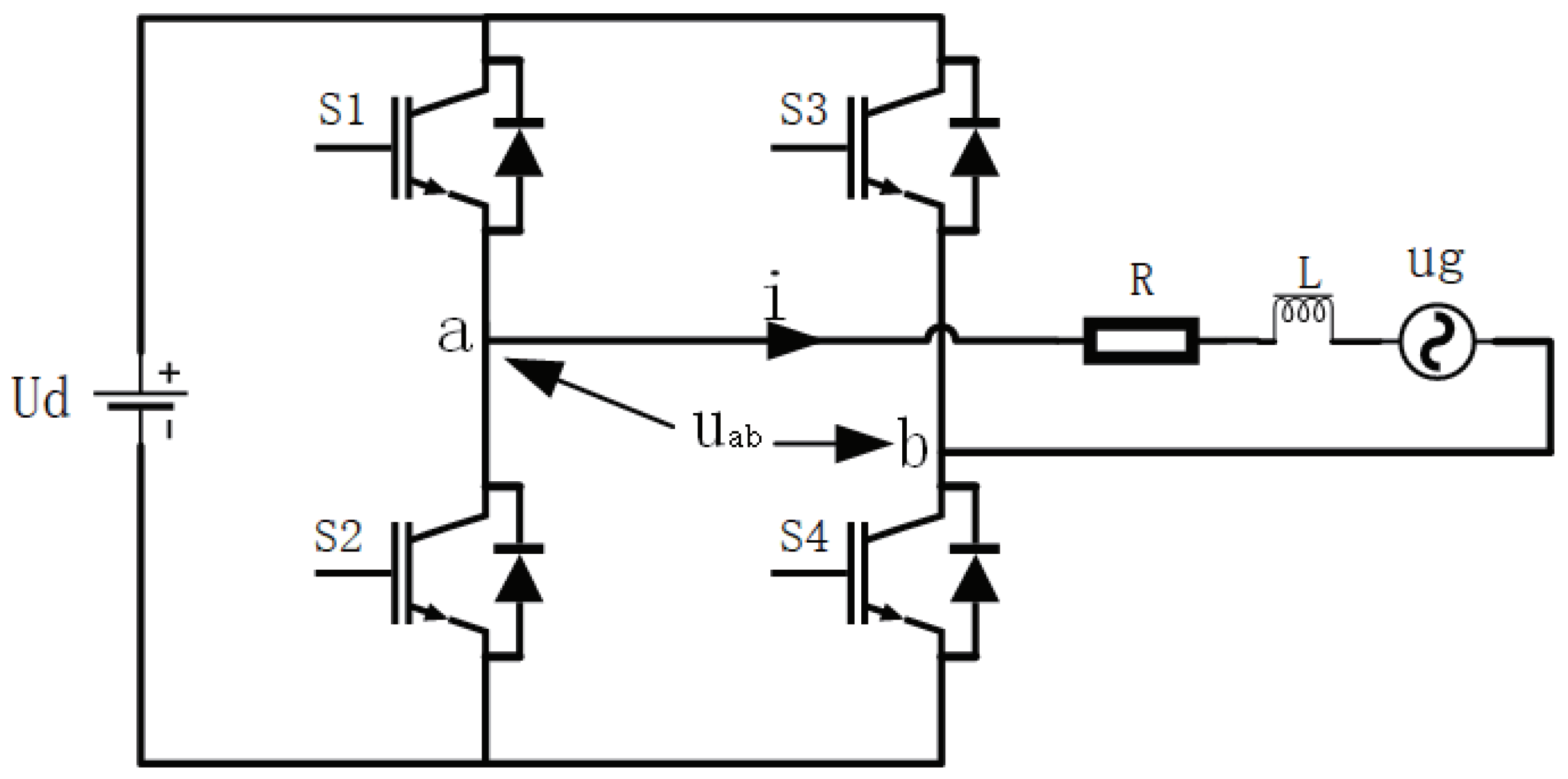
The typical single-phase inverter is presented in Figure 1, which is a well-known power electronics device employed for the conversion from DC electricity to AC. It consists of four power semiconductor switches named as S1–S4. Besides, it also contains the inductance L, resistance R and back electromotive force $u_g$. $i,U_d$ represent the output current and input DC voltage.

Note that the single-phase inverters can operate in three different operation modes, i.e., grid-feeding, grid-supporting and grid-forming modes [31]. In this paper, the grid connected inverter in this paper is operated in grid-feeding mode and the feedback is the output current i.

The continuous-time model of the inverter is obtained by Figure 1, expressed as:

$$\frac{di\left(t\right)}{dt}=-\frac{R}{L}i\left(t\right)+\frac{1}{L}\left[u_{ab}\left(t\right)-u_g\left(t\right)\right]$$

(1)

By applying forward Euler approximation [8], with $T_s$ as sampling time, the discrete form of Equation (1) is shown as:

$$i(k+1)=\left[1-\frac{R{T}_s}{L}\right]i\left(k\right)+\frac{T_s}{L}\left[u_{ab}\left(k\right)-u_g\left(k\right)\right]$$

(2)

where $u_{ab}\left(k\right)$ stands for the bridge voltage, which is described as $u_{ab}\left(k\right)=S\left(k\right)U_d$. $S\left(k\right)\in \{-1,0,1\}$ is the main operating states of the inverter and its value is determined by the switching state of four semiconductor units S1–S4.

It is known that each switch has two states, on and off. The switches in the same leg, namely $S1,S2$ or $S3,S4$, are working in complementary separately. When $S1$ is switched off and $S3$ is switched on, the value of $S\left(k\right)$ is $-1$. Conversely, it is changed to 1. $S\left(k\right)=0$ means that $S1$ and $S3$ are both switched off/on. Then, the bridge voltage $u_{ab}\left(k\right)$ contains the voltage levels of $\{-U_d,0,U_d\}$ corresponding to $S\left(k\right)=-1,0,1$.

2.2. Problem Statement

In steady state, the output of current $i\left(t\right)$ in Figure 1 can be expressed by using Fourier series as:

$$i\left(t\right)=I_0+\sum _{n=1}^{\infty }{A}_{n}sin\left(n\omega t\right)+\sum _{n=1}^{\infty }{B}_{n}cos\left(n\omega t\right)$$

(3)

where $n=1,2,3,4,\cdots$ is the harmonic order. The nth harmonic root mean square (RMS) value $I_n$ can be calculated by Equation (4).

$$I_n=\sqrt{\frac{A_n^2+B_n^2}{2}}$$

(4)

THD is widely used in evaluating the quality of AC power, and how to minimize THD is very important for the control of inverters. In [1], THD is defined as follows:

$$\mathrm{THD}=\frac{\sqrt{{\sum }_{n=2}^{\infty }{\left(I_n\right)}^2}}{I_1}$$

(5)

Note that Equation (5) needs each nth Fourier coefficients to calculate THD, and it requires many elements that are not suitable for real application. In reality, THD can also be calculated by another equivalent method, as defined in Equation (6) [1]:

$$\mathrm{THD}=\sqrt{\frac{I_{RMS}^2-I_0^2-I_1^2}{I_1^2}}$$

(6)

where $I_{RMS}$ is the RMS value of current i.

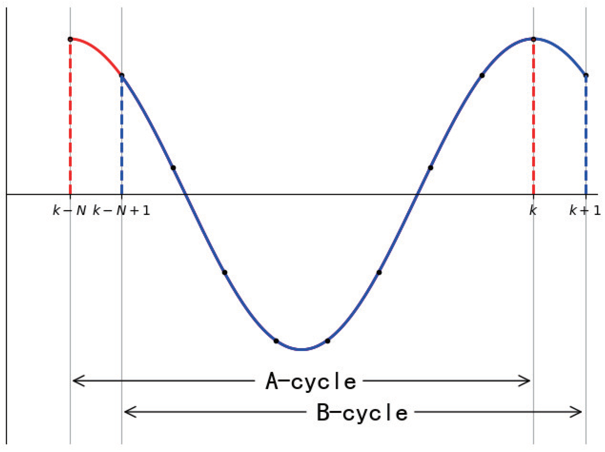
It is clear that the harmonics of current are almost the same in single or multiple fundamental period. Hence, in this paper, the THD optimization is conducted in a fundamental cycle (i.e., 0.02 s corresponding to 50 Hz) for simplicity, as illustrated in Figure 2. In this figure, A-cycle and B-cycle represent different cycles of adjacent points, and, in one cycle, the number of sampling points is described as N. In A-cycle, the DC, fundamental and THD values THD at kth point can be calculated, which are expressed as $I_0\left(k\right)$, $i_{\alpha }\left(k\right)$ and $THD\left(k\right)$. Similarly, $THD(k+1)$, $i_{\alpha }(k+1)$ and $I_0(k+1)$ are calculated from the B-cycle.

Theoretically, DC bias, fundamental wave and high-order harmonics are the main component of periodic signals. The primary control objectives for inverters are to reduce the tracking error of the fundamental component, eliminate the harmonics and guarantee less DC bias. In this paper, minimizing THD is the purpose of the proposed control scheme, and the tracking error and DC bias should be subject to special constraints. The optimization model to illustrate the control problem is presented as:

$$\begin{array}{c}\underset{S\left(k\right)}{min}y=[f1,f2,f3]\hfill \\ s.t.\left\{\begin{array}{c}f1=THD(k+1)\hfill \\ f2=|i_{\alpha }(k+1)-i^{*}(k+1)|\hfill \\ f3=|I_0(k+1)|\hfill \end{array}\right.\hfill \end{array}$$

(7)

3. Controller Design

3.1. Control Scheme

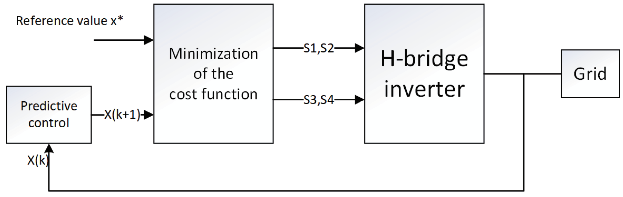
The scheme of the proposed THD-oriented FCS MPC method for grid connected inverters is presented in Figure 3. It is clear that this scheme is constructed based on the traditional FCS MPC method, where the major difference is the structure of the cost function. In this figure, the predictive control means predicting $X(k+1)$ at $(k+1)$th point under different switching combinations using the measured $X\left(k\right)$, mainly the output current $i\left(k\right)$ in this paper. Note that the measured values are obtained by sensors and the prediction is based on the system model. Then, the cost function calculation is conducted with every predicted value and the reference value. After that, the switching states are selected by minimizing the cost function and the corresponding switching signals are sent to the H-bridge inverters to achieve the control goals. In the experiment, the calculations were conducted in the FPGA module. The details are presented below.

3.2. THD Prediction

According to Equation (6), it is obvious that $I_{RMS}\left(k\right)$, $I_0\left(k\right)$, and $I_1\left(k\right)$ are the main factors deciding $THD\left(k\right)$ for discrete system. To avoid complexity, the THD is obtained by online iterative calculation described as follows.

$I_{RMS}\left(t\right),I_0\left(t\right)$ and $I_1\left(t\right)$ are easy to obtain for the continuous system, which are shown as:

$$I_{RMS}\left(t\right)=\sqrt{\frac{1}{T}{\int }_{t-T}^t{i}^2\left(x\right)\mathrm{d}x}$$

(8)

$$I_0\left(t\right)=\frac{1}{T}{\int }_{t-T}^{t}i\left(x\right)\mathrm{d}x$$

(9)

$$I_1\left(t\right)=\sqrt{\frac{A_1^2\left(t\right)+B_1^2\left(t\right)}{2}}$$

(10)

In Equation (10), $A_1\left(t\right),B_1\left(t\right)$ are defined by:

$$A_1\left(t\right)=\frac{2}{T}{\int }_{t-T}^{t}i\left(x\right)sin\left(\omega x\right)\mathrm{d}x$$

(11)

$$B_1\left(t\right)=\frac{2}{T}{\int }_{t-T}^{t}i\left(x\right)cos\left(\omega x\right)\mathrm{d}x$$

(12)

where $\omega$ is the fundamental angular frequency.

Then, from Equation (8), $I_{RMS}\left(k\right)$ for discrete system can be expressed as:

$$I_{RMS}\left(k\right)=\sqrt{\frac{1}{N}\sum _{j=k-N+1}^k{i}^2\left(j\right)}$$

(13)

The previous value $I_{RMS}(k-1)$ can be easily acquired by replacing k with $k-1$ in Equation (13). Substituting $I_{RMS}(k-1)$ into Equation (13), the recursive form of $I_{RMS}\left(k\right)$ is written as:

$$I_{RMS}^2\left(k\right)=I_{RMS}^2(k-1)+\frac{1}{N}[i^2\left(k\right)-i^2(k-N)]$$

(14)

In a similar way, Equations (9)–(12) are rewritten as

$$I_0\left(k\right)=I_0(k-1)+▵i\left(k\right)$$

(15)

$$I_1\left(k\right)=\sqrt{\frac{A_1^2\left(k\right)+B_1^2\left(k\right)}{2}}$$

(16)

$$A_1\left(k\right)=A_1(k-1)+2▵i\left(k\right)sin\left(\frac{2\pi }{N}k\right)$$

(17)

$$B_1\left(k\right)=B_1(k-1)+2▵i\left(k\right)cos\left(\frac{2\pi }{N}k\right)$$

(18)

where $▵i\left(k\right)=\frac{1}{N}[i\left(k\right)-i(k-N)]$.

The formulas above illustrate the iterative calculation process of $THD\left(k\right)$. Similarly, by applying the same method with $\widehat{i}(k+1)$ and $i(k-N+1)$, the predictive value $\widehat{THD}(k+1)$ can be easily obtained for FCS MPC design.

3.3. Fundamental Wave Extraction

For periodic signals, a direct way to extract fundamental wave is by multiplying the original signal by the standard cosine function, as shown in Equation (19).

$$i_1\left(t\right)=\frac{2}{T}{\int }_{x=t-T}^{t}i\left(x\right)cos\left[\omega \right(x-t+T\left)\right]dx$$

(19)

where the $i_1\left(t\right)$ is the instantaneous fundamental value of current $i\left(t\right)$.

However, the difficulties of rewriting Equation (19) in recursive form have restricted its application. In reality, digital filters have commonly been used in many cases and the Second Order Generalized Integrator (SOGI) can extract the fundamental signal quickly [32].

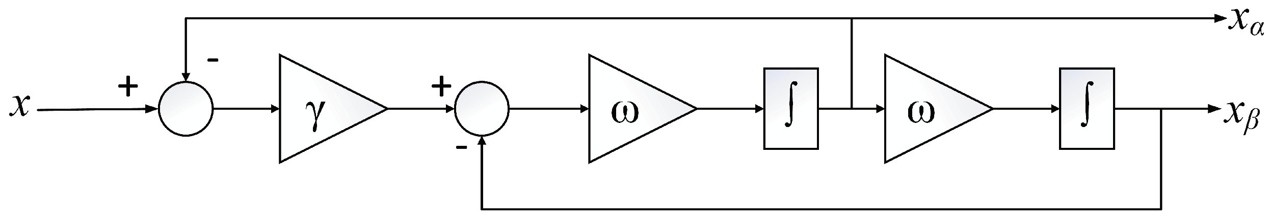
The basic structure of SOGI is illustrated in Figure 4. Except for the central frequency $\omega$, the damping factor $\gamma$ is also contained in the scheme, which can impact the influence of SOGI. The SOGI can filter the harmonics being away from $\omega$. The acquisition of discrete-time integrator is important for the discrete implementation of SOGI. Using the forward Euler method for integrator estimating, the SOGI can be written as follow:

$$\begin{array}{c}\hfill \left\{\begin{array}{c}{i}_{\alpha }\left(k\right)=(1-\gamma \omega T_s)i_{\alpha }(k-1)+\omega T_s[\gamma i\left(k\right)-i_{\beta }(k-1)]\hfill \\ i_{\beta }\left(k\right)=i_{\beta }(k-1)+\omega T_s{i}_{\alpha }(k-1)\hfill \end{array}\right.\end{array}$$

(20)

3.4. FCS MPC Scheme

To drive the switching units for inverters current tracking, FCS MPC scheme is used to determine the appropriate switching states judged by the cost function. It should be noted that, for MPC, the future control sequence is obtained by minimizing the cost function used to evaluate the predicted values and it applies the first value of the sequence to converters. However, FCS MPC is implemented by predicting and applying the future values to the cost function corresponding to every switching states and then selecting the associate switching states with minimum cost function. Since there are finite switching states for power converters, FCS MPC is widely and successfully employed in the converters control.

The implementation process is mainly divided into three steps. Firstly, the predicted current is obtained by the discrete model of single-phase inverters in Equation (2), shown as:

$${\widehat{i}}_x(k+1)=\left[1-\frac{R{T}_s}{L}\right]i\left(k\right)+\frac{T_s}{L}\left[S_x{U}_d-u_g\left(k\right)\right]$$

(21)

where $S_x$ and ${\widehat{i}}_x(k+1)$ are the xth switching combination and corresponding predicted current. As mentioned above, $S_x\in \{-1,0,1\}$, which means the subscript $x\in \{1,2,3\}$.

Hence, according to Equations (6), (15) and (20), the predicted current fundamental values, THD and DC values are described as

$${\widehat{i}}_{\alpha ,x}(k+1)=(1-\gamma \omega T_s)i_{\alpha }\left(k\right)+\omega T_s[\gamma {\widehat{i}}_x(k+1)-i_{\beta }\left(k\right)]$$

(22)

$${\widehat{THD}}_x(k+1)=\sqrt{\frac{{\widehat{I}}_{RMS,x}^2(k+1)-{\widehat{I}}_{0,x}^2(k+1)-{\widehat{I}}_1^2(k+1)}{{\widehat{I}}_{1,x}^2(k+1)}}$$

(23)

$${\widehat{I}}_{0,x}(k+1)=I_0\left(k\right)+▵{\widehat{i}}_x(k+1)$$

(24)

where $i_{\beta }\left(k\right),{\widehat{I}}_{RMS,x}(k+1),{\widehat{I}}_{1,x}(k+1)$ are obtained by Equations (14), (16)–(18) and (20). The symbol $\widehat{|·|}$ means the predicted current ${\widehat{i}}_x(k+1)$ is used.

Secondly, the cost function is deduced by the given reference and the predicted values. In this paper, one step FCS MPC is employed to avoid the complex calculations, where the conventional form for inverters is expressed as:

$$J_x=|{\widehat{i}}_x(k+1)-i^{*}(k+1)|$$

(25)

where $i^{*}(k+1)$ is the reference value at $(k+1)$th point.

Then, for the proposed THD oriented FCS MPC, the cost function is modified to satisfy the objectives in Equation (7). The weights ${\lambda }_1$ and ${\lambda }_2$ are introduced to turn the problems into a single-objective optimization problem. The modified cost function is reconstructed by the weighted summation of the error between the reference values and the predicted fundamental values of output current, the predicted THD value and the predicted DC component of output current, which is presented as:

$$J_x=|{\widehat{i}}_{\alpha ,x}(k+1)-i^{*}(k+1)|+{\lambda }_1{\widehat{THD}}_x(k+1)+{\lambda }_2\left|{\widehat{I}}_{0,x}(k+1)\right|$$

(26)

Finally, comparing the cost $J_x$, the optimal $S\left(k\right)$ can be obtained with the minimum associated cost, which is expressed as:

$$S\left(k\right)=S_x,when{J}_x=\underset{x\in \{1,2,3\}}{min}\left(J_x\right)$$

(27)

According to the relationship between $S\left(k\right)$ and the switching states of the semiconductor units S1–S4 mentioned in Section 2.1, the switching signals are generated to achieve the control objectives.

3.5. Close Loop Realization

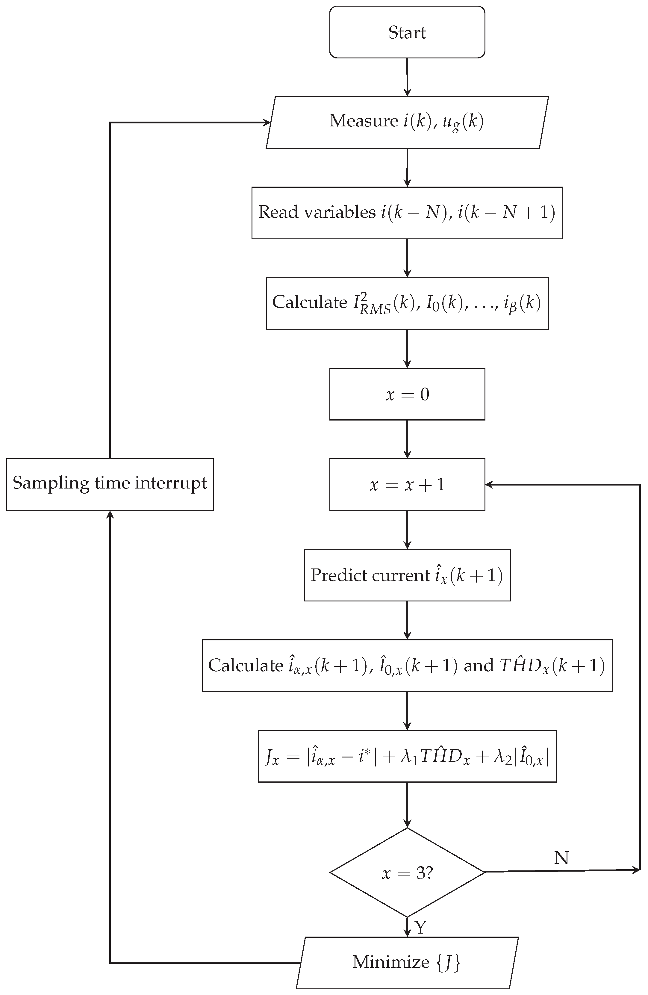
Figure 5 demonstrates the control algorithm of proposed method, where the operation steps are described as follows:

Step 1

Initialize digital controller.

Step 2

Measure $i\left(k\right)$ and $u_g\left(k\right)$ by sensors, and read $i(k-N),i(k-N+1)$ from memory.

Step 3

Calculate $I_{RMS}^2\left(k\right)$, $I_0\left(k\right)$, $A_1\left(k\right)$, $B_1\left(k\right)$, $i_{\alpha }\left(k\right)$ and $i_{\beta }\left(k\right)$ through Equations (14)–(18) and (20).

Step 4

Initialize the inner loop with $x=0$.

Step 5

Add 1 to cycle count value x, and select the xth switch state to calculate the corresponding predicted current $\widehat{i}(k+1)$.

Step 6

Use $\widehat{i}(k+1)$ to calculate ${\widehat{i}}_{\alpha }(k+1)$, $\widehat{THD}(k+1)$ and ${\widehat{I}}_0(k+1)$ according to Equations (22)–(24).

Step 7

Calculate the cost function $J_x$ by Equation (26).

Step 8

Judge $x=3$? If yes, then next step, else jump to Step 5.

Step 9

Select the optimal $S\left(k\right)$ corresponding to the minimum cost J, then send the switching signals to inverters and return to Step 2.

It should be noted that the control algorithm was implemented by Stateflow block of Matlab/Simulink in simulation and by programming the FPGA module of NI compactRIO 9033 in experiment. The details are illustrated in Section 4 and Section 5.

4. Simulation Verification

To confirm the effectiveness of proposed controller, a single-phase inverter model, i.e., the model shown in Figure 1, was established in Matlab/Simulink for simulation with the presented parameters in

Table 1. Simulation parameters.

Parameters	Descriptions	Value
L	The filter inductance	5 mH
R	The ESR of L	1 Ω
$U_d$	The input DC voltage	48 V
$u_g$	The back electromotive force	20 $sin{\omega }_{0}t$(V)
$f_0$	The output AC frequency	50 Hz
$f_s$	The control sampling frequency	10 kHz

. Note that Stateflow block was used for the control algorithm programming and generating the switching signals to drive the switching units, where the steps are elaborated in Section 3.5.

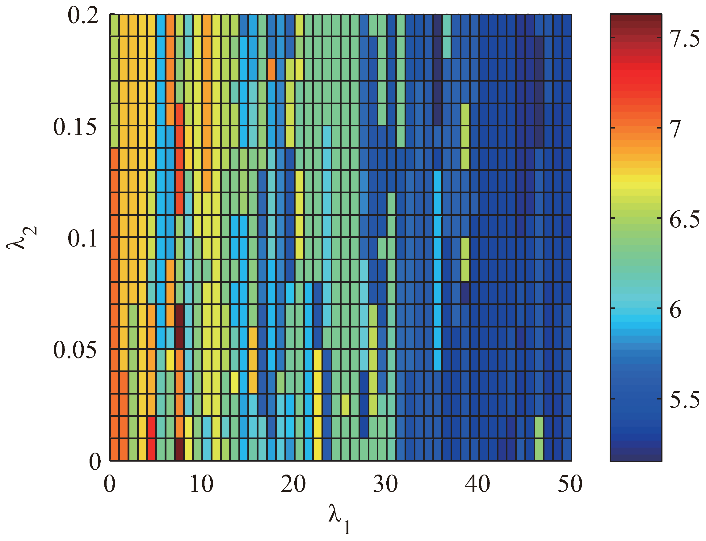
Since the selection of weights ${\lambda }_1$, ${\lambda }_2$ plays an important role in the realization of proposed controller, a group of simulations were carried out with ${\lambda }_1=[1,\dots ,50],{\lambda }_2=[0,\dots ,0.2],i^{*}=6sin{\omega }_{0}t\left(A\right)$, where ${\omega }_0=2\pi f_0$ to show the change of THD in steady-state, as presented in Figure 6.

As illustrated in Figure 6, the performance is related to both ${\lambda }_1$ and ${\lambda }_2$, especially sensitive to ${\lambda }_1$. According to the analysis, the minimum of THD in Figure 6 is 5.1708% when ${\lambda }_1=46,{\lambda }_2=0.14$. Under the same circumstance, the THD of traditional FCS MPC is 5.6814%. In other words, the minimum value of THD at this condition is reduced by 8.9877% compared with the traditional one.

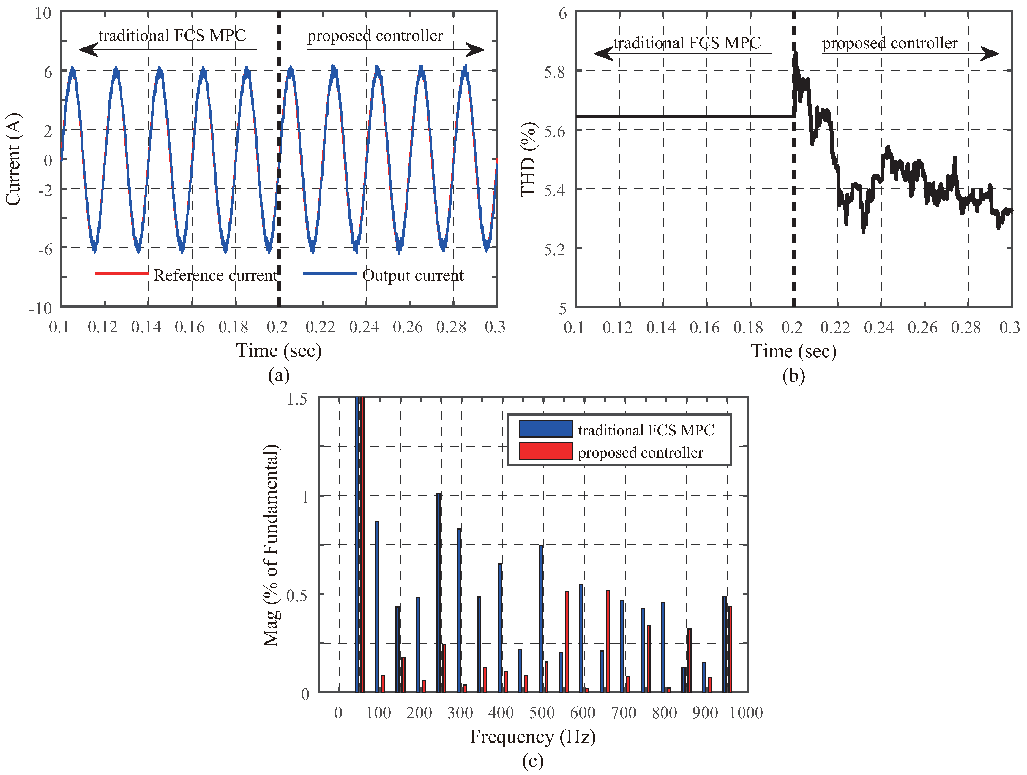
The tracking effects of two methods under same reference signal, namely, $i^{*}=6sin{\omega }_{0}t\left(A\right)$, are shown in Figure 7. In the figure, the transit time from traditional FCS MPC to proposed controller is set to 0.2 s, as presented in Figure 7a. The dynamic change process of THD is shown in Figure 7b, indicating that the THD of proposed controller is lower compared with traditional FCS MPC. In addition, the harmonic analysis in Figure 7c also presents that most of the harmonic components of proposed controller are lower than the traditional one, which is the explanation for the decrease of THD. It should be noted that the average times of switching in one second for proposed controller is 3000 while that for traditional FCS MPC is 3400, which means there are no bad effects on switching.

5. Experimental Verification

5.1. Test Bench

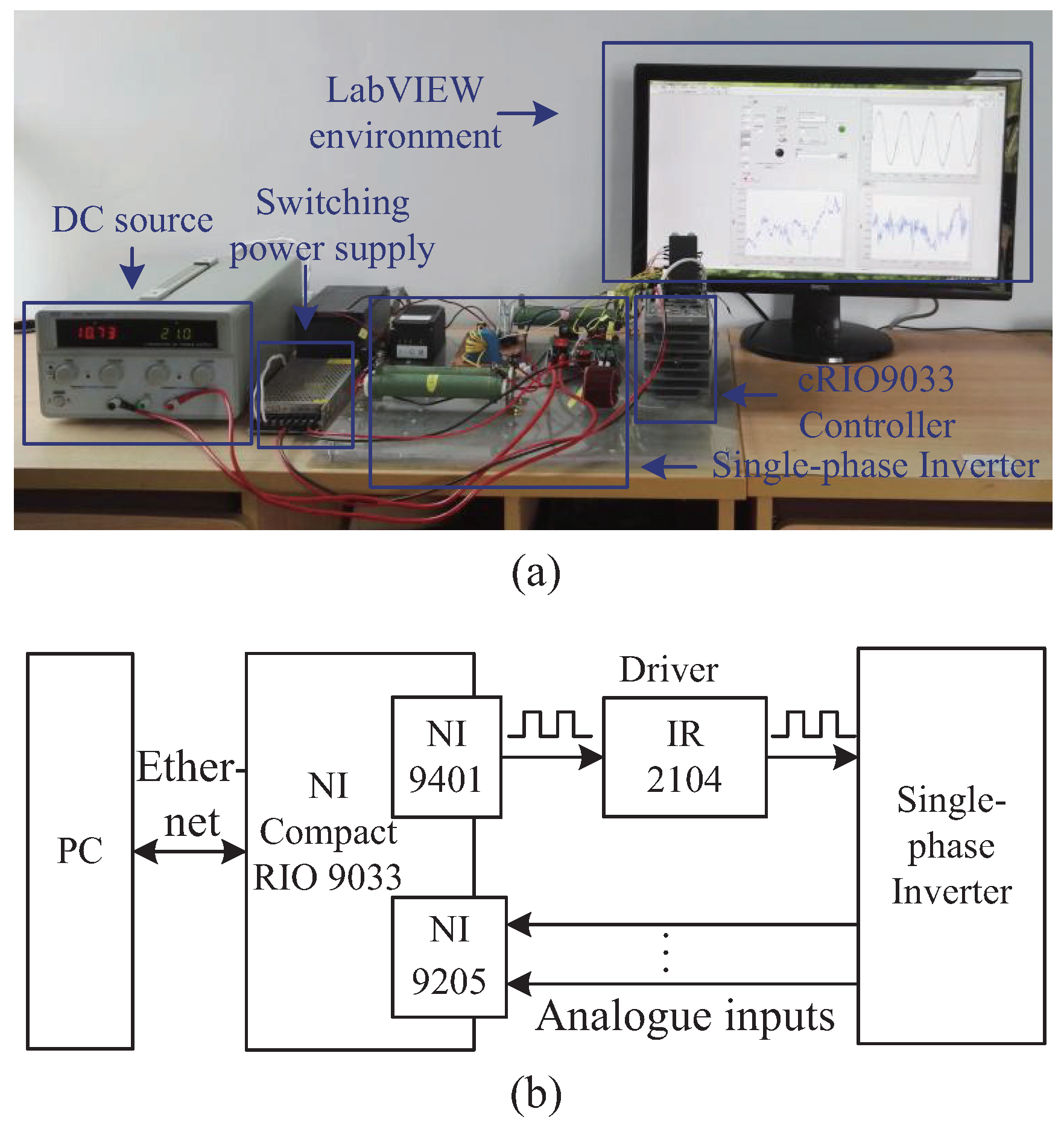
An experimental platform of single-phase inverters was implemented to further validate the proposed controller presented in Figure 8a. Figure 8b illustrates how the platform works by a block diagram and the specifications are listed in

Table 2. Experimental platform design parameters.

Parameter	Model
Controller	NI compactRIO 9033
Acquisition card	NI 9205
Execution unit	NI 9401
Current sensor	LAH50-P
Isolation IC	74HC244
Gate Driver IC	IR2104
Switch tube	IPB044N15N5
DC source	MPS-6010LP-1
Switching power supply	D-220DC 24 V/12 V

.

The test bench is mainly made up of LabVIEW interface, embedded NI CompactRIO 9033, single-phase inverter circuit, DC source and current sensor. As for NI cRIO 9033, the main component is a FPGA module as an important part for the implementation and execution of proposed control law. Then, NI 9205 is a 16-bit analog input module with 32 single-ended or 16 differential channels, which is used to measure output current of the circuit. Its maximum input range and sampling rates are ±10 V and 250 kS/s, respectively. A digital input/output module NI 9401 was used to output control signals, via one of its eight bidirectional channels, to achieve control objectives, and the updating rate is 100 ns. Both NI 9205 and NI 9401 are connected to the FPGA module of NI cRIO 9033 by high-speed internal bus. Note that the LabVIEW environment in PC, communicating with NI cRIO 9033 via ethernet, helps to program FPGA module, and save and check the experimental results for better demonstration, similar to a man–machine interface.

5.2. Experimental Results

According to the control algorithm in Section 3.5, experiments were conducted on the platform presented in Figure 8, where

Table 3. Experimental parameters.

Parameters	Descriptions	Value
L	The load inductance	6.085 mH
R	The load resistance	5.46 Ω
$U_d$	The input DC voltage	21 V
$u_g$	The back electromotive force	0 V
$f_0$	The output AC frequency	50 Hz
$f_s$	The control sampling frequency	10 kHz

lists the parameters. NI cRIO 9033 was used as the controller with the FPGA module programmed by LabVIEW. Besides, the comparison between traditional FCS MPC and proposed controller is also demonstrated. Note that the back electromotive force $u_g$ is set to 0 due to the test bench.

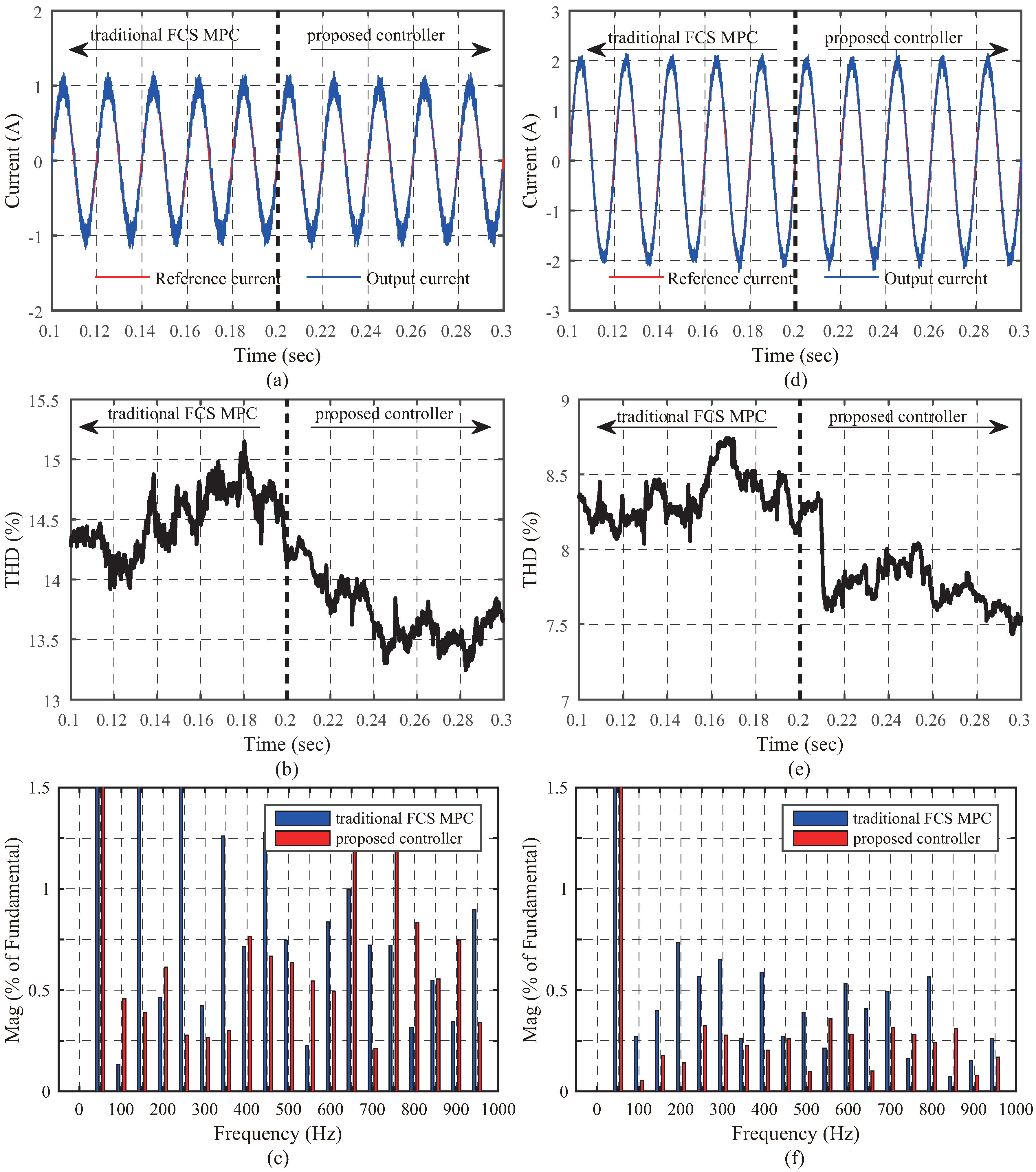
Figure 9 demonstrates the performance of traditional FCS MPC and proposed controller with $i^{*}=1sin{\omega }_{0}t\left(A\right)$ and $i^{*}=2sin{\omega }_{0}t\left(A\right)$. Taking $i^{*}=2sin{\omega }_{0}t\left(A\right)$ as an example, from $t=0.1$ s to $t=0.2$ s, traditional FCS MPC was used for the current tracking, while the proposed method was applied after $t=0.2$ s in Figure 9d. It can be easily found that the instantaneous THD value was reduced significantly after $t=0.2$ s in Figure 9e. Besides, through FFT analysis shown in Figure 9f of current waveform in the steady state, a lower magnitude in most harmonic components can be obtained by proposed method compared with traditional FCS MPC, which was similar to the simulation. By comparing the waveform and the THD performance, it was found that a lower THD (8.00%) was obtained from proposed controller while that from traditional FCS MPC was 8.21%, and the decline was about 2.56%. As for $i^{*}=1sin{\omega }_{0}t\left(A\right)$, there are similar results in Figure 9a–c. It should be noted that, compared with the simulations, the improvement of THD was a little lower, which may be resulted from the noise of current sensor and the time-delay from calculation.

Table 4. THD in different current.

i* (A)	${\mathit{\lambda }}_1$	${\mathit{\lambda }}_2$	THD1 (%) a	THD2 (%) b	Decline (%)
1$sin{\omega }_{0}t$	2.6	0.03	14.60	13.71	6.08
2$sin{\omega }_{0}t$	7.0	0.05	8.21	8.00	2.56
3$sin{\omega }_{0}t$	15.0	0.07	6.27	6.20	1.12
4$sin{\omega }_{0}t$	32.0	0.10	4.93	4.88	1.01

^a The THD of traditional FCS MPC; ^b The THD of proposed controller.

presents the improvements of THD with different $i^{*}$ to further verify the effectiveness of the proposed controller, where the weights ${\lambda }_1$ and ${\lambda }_2$ were selected by offline optimization. It can be easily found that, compared with the traditional FCS MPC, the performance of proposed controller was better. The THD was reduced overall, especially when tracking low current. Meanwhile, the calculation time for proposed controller was 6.125 µs (245 ticks at 40 MHz clock) while it was 5.05 µs (202 ticks at 40 MHz clock) for traditional FCS MPC in this paper, indicting that the computation burden for proposed method was a little larger. However, there was no bad effect on the control performance.

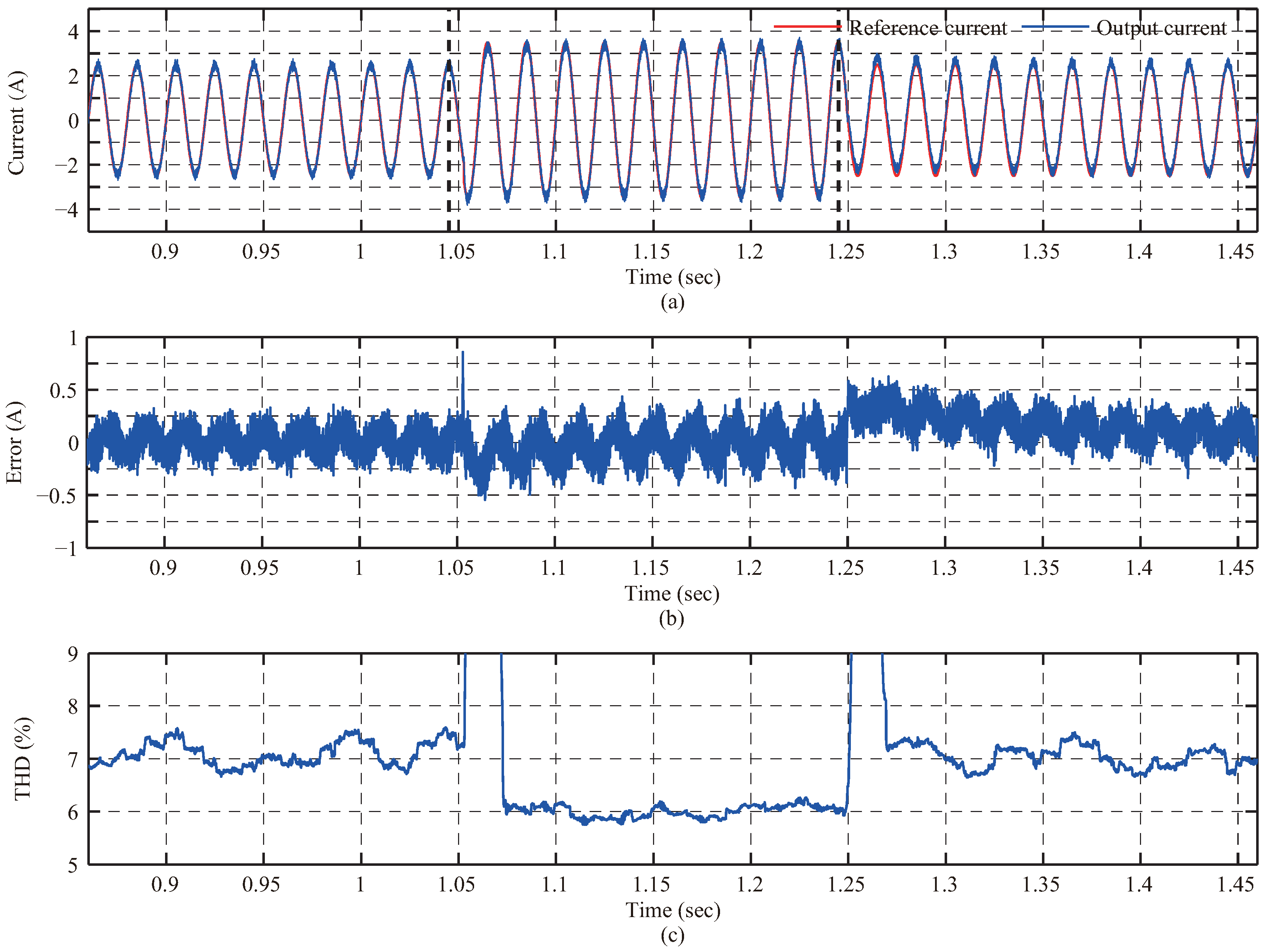
In addition, the instant response of proposed controller is displayed in Figure 10. At about 1.045 s, shown by the bold dotted line in the figure, the reference current changed from 2.5 A to 3.5 A, and the output current tracked the reference rapidly as well as the descending process. As for the tracking error, a sudden increase can be seen at the changing moment and it decreased to a reasonable range quickly. As shown in Figure 10c, THD had a large mutation when $i^{*}$ changed. Then, after a period, it dropped to normal value and gradually restores to stable status.

6. Conclusions

In this paper, concerned with the real-time THD control, a THD oriented FCS MPC controller is designed for single-phase inverters. Reducing THD has always been the focus of inverter control, but the real-time control using THD as a direct object has not been widely studied before. FCS MPC is characterized by its simplicity and the ability to process various control objectives. Hence, the control problem for proposed method is formulated as a multi-objective optimization problem. To achieve this goal, the cost function is modified to handle this problem, which is constructed by the linear combination with weight factors of the current fundamental tracking error, instantaneous THD value and DC component. Besides, iterative method is developed to reduce the computational burden. Simulations and experiments were conducted to verify the effectiveness of proposed method. The results indicate that, compared with traditional FCS MPC, better performance can be obtained, especially when tracking low current, and there is no obvious increase in the calculation time. Note that appropriate weights make the proposed controller perform well in THD reduction, while abusing weights may lead to bad performance becoming even worse. In other words, good weights can make a difference when the operation condition changes, such as the reference current amplitude and circuit parameters, which need further research.

References

- Dordevic, O.; Jones, M.; Levi, E. Analytical Formulas for Phase Voltage RMS Squared and THD in PWM Multiphase Systems. IEEE Trans. Power Electron. 2015, 30, 1645–1656. [Google Scholar] [CrossRef] [Green Version]
- Zhong, Q.C.; Hornik, T. Cascaded Current-Voltage Control to Improve the Power Quality for a Grid-Connected Inverter with a Local Load. IEEE Trans. Ind. Electron. 2013, 60, 1344–1355. [Google Scholar] [CrossRef]
- Chen, D.; Zhang, J.; Qian, Z. An Improved Repetitive Control Scheme for Grid-Connected Inverter with Frequency-Adaptive Capability. IEEE Trans. Ind. Electron. 2013, 60, 814–823. [Google Scholar] [CrossRef]
- Noman, A.M.; Al-Shamma’a, A.A.; Addoweesh, K.E.; Alabduljabbar, A.A.; Alolah, A.I. Cascaded Multilevel Inverter Topology Based on Cascaded H-Bridge Multilevel Inverter. Energies 2018, 11, 895. [Google Scholar] [CrossRef]
- Franquelo, L.G.; Rodriguez, J.; Leon, J.I.; Kouro, S. The age of multilevel converters arrives. IEEE Ind. Electron. Mag. 2008, 2, 28–39. [Google Scholar] [CrossRef]
- Alishah, R.S.; Nazarpour, D.; Hosseini, S.H.; Sabahi, M. Reduction of Power Electronic Elements in Multilevel Converters Using a New Cascade Structure. IEEE Trans. Ind. Electron. 2015, 62, 256–269. [Google Scholar] [CrossRef]
- Jahani, F.; Monfared, M. A Multilevel AC/AC Converter with Reduced Number of Switches. IEEE Trans. Ind. Electron. 2018, 65, 1244–1253. [Google Scholar] [CrossRef]
- Metri, J.I.; Vahedi, H.; Kanaan, H.Y.; Al-Haddad, K. Real-Time Implementation of Model-Predictive Control on Seven-Level Packed U-Cell Inverter. IEEE Trans. Ind. Electron. 2016, 63, 4180–4186. [Google Scholar] [CrossRef] [Green Version]
- Jayalath, S.; Hanif, M. Generalized LCL-Filter Design Algorithm for Grid-Connected Voltage-Source Inverter. IEEE Trans. Ind. Electron. 2017, 64, 1905–1915. [Google Scholar] [CrossRef]
- Pandey, R.; Tripathi, R.N.; Hanamoto, T. Comprehensive Analysis of LCL Filter Interfaced Cascaded H-Bridge Multilevel Inverter-Based DSTATCOM. Energies 2017, 10, 346. [Google Scholar] [CrossRef]
- Liu, Y.; Lai, C.M. LCL Filter Design with EMI Noise Consideration for Grid-Connected Inverter. Energies 2018, 11, 1646. [Google Scholar] [CrossRef]
- Fang, J.; Li, X.; Yang, X.; Tang, Y. An Integrated Trap-LCL Filter with Reduced Current Harmonics for Grid-Connected Converters under Weak Grid Conditions. IEEE Trans. Power Electron. 2017, 32, 8446–8457. [Google Scholar] [CrossRef]
- Wu, W.; He, Y.; Blaabjerg, F. An LLCL Power Filter for Single-Phase Grid-Tied Inverter. IEEE Trans. Power Electron. 2012, 27, 782–789. [Google Scholar] [CrossRef]
- Napoles, J.; Leon, J.I.; Portillo, R.; Franquelo, L.G.; Aguirre, M.A. Selective harmonic mitigation technique for high-power converters. IEEE Trans. Ind. Electron. 2010, 57, 2315–2323. [Google Scholar] [CrossRef]
- Srndovic, M.; Zhetessov, A.; Alizadeh, T.; Familiant, Y.; Grandi, G.; Ruderman, A. Simultaneous Selective Harmonic Elimination and THD Minimization for a Single-Phase Multilevel Inverter with Staircase Modulation. IEEE Trans. Ind. Appl. 2018, 54, 1532–1541. [Google Scholar] [CrossRef]
- Ahmadi, D.; Zou, K.; Li, C.; Huang, Y.; Wang, J. A universal selective harmonic elimination method for high-power inverters. IEEE Trans. Power Electron. 2011, 26, 2734–2752. [Google Scholar] [CrossRef]
- Massrur, H.R.; Niknam, T.; Mardaneh, M.; Rajaei, A.H. Harmonic Elimination in Multilevel Inverters Under Unbalanced Voltages and Switching Deviation Using a New Stochastic Strategy. IEEE Trans. Ind. Inform. 2016, 12, 716–725. [Google Scholar] [CrossRef]
- Kavousi, A.; Vahidi, B.; Salehi, R.; Bakhshizadeh, M.K.; Farokhnia, N.; Fathi, S.H. Application of the Bee Algorithm for Selective Harmonic Elimination Strategy in Multilevel Inverters. IEEE Trans. Power Electron. 2012, 27, 1689–1696. [Google Scholar] [CrossRef]
- Shen, K.; Zhao, D.; Mei, J.; Tolbert, L.M.; Wang, J.; Ban, M.; Ji, Y.; Cai, X. Elimination of Harmonics in a Modular Multilevel Converter Using Particle Swarm Optimization-Based Staircase Modulation Strategy. IEEE Trans. Ind. Electron. 2014, 61, 5311–5322. [Google Scholar] [CrossRef]
- Yuan, J.; Pan, J.; Fei, W.; Cai, C.; Chen, Y.; Chen, B. An Immune-Algorithm-Based Space-Vector PWM Control Strategy in a Three-Phase Inverter. IEEE Trans. Ind. Electron. 2013, 60, 2084–2093. [Google Scholar] [CrossRef]
- Agarwal, P.; Agarwal, V. A novel approach of space vector modulation for cycloinverter using genetic algorithm. IET Power Electron. 2013, 6, 1723–1731. [Google Scholar] [CrossRef]
- Yang, S.H.; Yang, Y.H.; Chen, K.H.; Lin, Y.H.; Tsai, T.Y.; Lin, S.R.; Lee, C. A Low-THD Class-D Audio Amplifier with Dual-Level Dual-Phase Carrier Pulsewidth Modulation. IEEE Trans. Ind. Electron. 2015, 62, 7181–7190. [Google Scholar] [CrossRef]
- Coppola, M.; Napoli, F.D.; Guerriero, P.; Iannuzzi, D.; Daliento, S.; Pizzo, A.D. An FPGA-Based Advanced Control Strategy of a Grid-Tied PV CHB Inverter. IEEE Trans. Power Electron. 2016, 31, 806–816. [Google Scholar] [CrossRef]
- Attia, H.A.; Tan, K.S.F.; Hang, S.C.; Hew, W.P.; Khateb, A.E. Confined Band Variable Switching Frequency Pulse Width Modulation (CB-VSF PWM) for Single-Phase Inverter with LCL Filter. IEEE Trans. Power Electron. 2017, 32, 8593–8605. [Google Scholar] [CrossRef]
- Rajapakse, G.; Jayasinghe, S.; Fleming, A.; Negnevitsky, M. A Model Predictive Control-Based Power Converter System for Oscillating Water Column Wave Energy Converters. Energies 2017, 10, 1631. [Google Scholar] [CrossRef]
- Kouro, S.; Cortes, P.; Vargas, R.; Ammann, U.; Rodriguez, J. Model Predictive Control-A Simple and Powerful Method to Control Power Converters. IEEE Trans. Ind. Electron. 2009, 56, 1826–1838. [Google Scholar] [CrossRef]
- Kouro, S.; Perez, M.A.; Rodriguez, J.; Llor, A.M. Model Predictive Control: MPC’s Role in the Evolution of Power Electronics. IEEE Ind. Electron. Mag. 2015, 9, 8–21. [Google Scholar] [CrossRef]
- Aguilera, R.P.; Acuna, P.; Yu, Y.; Konstantinou, G.; Townsend, C.D.; Wu, B.; Agelidis, V.G. Predictive Control of Cascaded H-Bridge Converters Under Unbalanced Power Generation. IEEE Trans. Ind. Electron. 2017, 64, 4–13. [Google Scholar] [CrossRef] [Green Version]
- Rodríguez, J.; Pontt, J.; Silva, C.A.; Correa, P.; Lezana, P.; Cortés, P.; Ammann, U. Predictive current control of a voltage source inverter. IEEE Trans. Ind. Electron. 2007, 54, 495–503. [Google Scholar] [CrossRef]
- Bayhan, S.; Trabelsi, M.; Abu-Rub, H.; Malinowski, M. Finite-Control-Set Model-Predictive Control for a Quasi-Z-Source Four-Leg Inverter Under Unbalanced Load Condition. IEEE Trans. Ind. Electron. 2017, 64, 2560–2569. [Google Scholar] [CrossRef]
- Viinamäki, J.; Kuperman, A.; Suntio, T. Grid-Forming-Mode Operation of Boost-Power-Stage Converter in PV-Generator-Interfacing Applications. Energies 2017, 10, 1033. [Google Scholar] [CrossRef]
- Monfared, M.; Sanatkar, M.; Golestan, S. Direct active and reactive power control of single-phase grid-tie converters. IET Power Electron. 2012, 5, 1544–1550. [Google Scholar] [CrossRef]
Figure 1.
The topology of single-phase inverters.
Figure 2.
Cycles selecting illustrate.
Figure 3.
General scheme for proposed method.
Figure 4.
Scheme for Second Order Generalized Integrator (SOGI).
Figure 5.
Control Algorithm.
Figure 6.
THD performance of different weights.
Figure 7.
Simulation results of two methods: (a) output current; (b) THD; and (c) harmonic analysis.
Figure 8.
Rapid control prototype: (a) experimental platform; and (b) block diagram.
Figure 9.
Experimental results of two methods: (a) output current with ; (b) THD with ; (c) harmonic analysis with ; (d) output current with ; (e) THD with ; and (f) harmonic analysis with .
Figure 10.
Instant response of proposed controller: (a) output current; (b) error; and (c) THD.