Short-Term Forecasting of Total Energy Consumption for India-A Black Box Based Approach


1
Institute for Energy Studies, Anna University, Chennai 600025, India
2
Department of Education, Gandhigram Rural Institute, Dindigul 624302, India
*
Author to whom correspondence should be addressed.
Energies 2018, 11(12), 3442; https://doi.org/10.3390/en11123442
Submission received: 31 October 2018
/
Revised: 29 November 2018
/
Accepted: 29 November 2018
/
Published: 9 December 2018
(This article belongs to the Special Issue Short-Term Load Forecasting by Artificial Intelligent Technologies)
Abstract
:Continual energy availability is one of the prime inputs requisite for the persistent growth of any country. This becomes even more important for a country like India, which is one of the rapidly developing economies. Therefore electrical energy’s short-term demand forecasting is an essential step in the process of energy planning. The intent of this article is to predict the Total Electricity Consumption (TEC) in industry, agriculture, domestic, commercial, traction railways and other sectors of India for 2030. The methodology includes the familiar black-box approaches for forecasting namely multiple linear regression (MLR), simple regression model (SRM) along with correlation, exponential smoothing, Holt’s, Brown’s and expert model with the input variables population, GDP and GDP per capita using the software used are IBM SPSS Statistics 20 and Microsoft Excel 1997–2003 Worksheet. The input factors namely GDP, population and GDP per capita were taken into consideration. Analyses were also carried out to find the important variables influencing the energy consumption pattern. Several models such as Brown’s model, Holt’s model, Expert model and damped trend model were analysed. The TEC for the years 2019, 2024 and 2030 were forecasted to be 1,162,453 MW, 1,442,410 MW and 1,778,358 MW respectively. When compared with Population, GDP per capita, it is concluded that GDP foresees TEC better. The forecasting of total electricity consumption for the year 2030–2031 for India is found to be 1834349 MW. Therefore energy planning of a country relies heavily upon precise proper demand forecasting. Precise forecasting is one of the major challenges to manage in the energy sector of any nation. Moreover forecasts are important for the effective formulation of energy laws and policies in order to conserve the natural resources, protect the ecosystem, promote the nation’s economy and protect the health and safety of the society.
1. Introduction
Energy is the driving force of any nation. Energy security and energy efficiency is the need of the hour. Energy conservation, decentralized energy planning techniques seems to be the solution to meet the energy requirements in almost every sector. The installed capacity out of renewable energy during 2012–2013 was around 12.26% and now later during 2017–2018 it has come to around 18.8% (www.cea.nic.in) [1]. If this trend stays, it is anticipated that the renewable energy sources would come forward to contribute even more in near future, which is a good sign. Renewable energy sector is expanding rapidly and in particular it has already grabbed its attention to be the potential contributor for sustainable energy security. India is one among the mainly swiftly developing countries in the planet. Flourishing industrialization also requires energy to excel, which in turn makes India an energy starving state. At present India depends heavily upon the fossil fuels and also has to expend more, whereas India also has a huge potential for the alternative sources of energy [2]. India is almost certainly urbanizing quicker. With a severe development predicament in the energy sector, energy becomes one of the top focus and an additional major issue in sustainable improvement and also a long-term security [3]. Managing energy consumption and energy resources in parallel has become very important among energy planners and policy framers. Thus an incorporated energy administration approach is vital for the sustainable improvement of India. Models have turned out to be the standard tools in energy planning. For energy modelling, energy forecasting is a basic necessary requirement. This emphasizes the significance of energy forecasting. Demand forecast is similarly a vital job for the effectual function and setting up of systems. Forecasts can be catalogued as long-term, medium and short-term depending upon the time. Long-term prediction, generally keep up a correspondence to several months to even several decades to the front. Overvalued electricity and energy consumption forecast will result in heedless venture in the erection of surplus power amenities and other inventories; whereas undervaluing the consumption might end up with deficient manufacturing, planning and will not be able to bridge the gap with the demand. Short term forecasting always draws attention and it is also paying attention in point forecasts. Density forecasts that is, forecasts that provide approximation of the probability distributions of the likely upcoming values of the consumption be essential for long-term forecast. In the literature a range of forecasting practices has been witnessed in the earlier period, generally presumptuous short and midterm forecasts. To assess the execution of the comparative study the real and forecasted results are figured out and the forecasts based upon the data observed up to 2017 are also worked out. The outcome proves good foreseeing capability of the proposed method at forecasting the country’s energy consumption.
The literature is actually huge with the number of competing models and some major contributions among them are read. In support of perspective of single day or with a reduction in it, models employing univariate time series models [4,5] and ANN [6] are quite familiar. Some of the researchers have used forecasting models and techniques. Several forecasting methods were used in energy forecasting leading to different levels of accomplishment. Starting from linear regression, multi-variate regression and so on, several other models have also been used [7,8,9]. Time series models for various years have been offered with multinomial, linear and also exponential approximation [10].
Mixed Integer Linear Programming model has been evolved for the optimized electricity generation scheme planning for the country to reach a precise CO2 emission target [11]. Holt’s method was used to determine three different circumstances such as business as usual, renewable energy and also regarding how to conserve energy [12]. Long-term dynamic linear programming model was considered to calculate future investments of electricity production technologies of very long-term energy scenarios. Linear Programming (LP) can be implemented to support the choice of renewable energy technology to meet CO2 emission reduction targets [13]. An estimation of data-driven models was performed by Tardioli et al. at city level [14]. Choi et al. offers an extreme deep learning method to obtain improved building energy consumption forecast [15].
Simple fuzzy models incorporating Artificial Intelligence techniques have been useful to forecast midterm energy and also the peak load [16,17,18]. A new way of energy demand forecasting at an intra-day ruling using semi parametric regression smoothing which relates for the yearly and weather conditional components is suggested. Dependence upon the residual series is explained by one among the two multiple variables time series models, with the measurement identical to the quantity of intra-day range. The profit of this procedure in the process of forecasting of: (i) Demand for heating steam network of one of the district in Germany; (ii) collective electricity demand in Victoria, a state in Australia. With both studies accounting for meteorological conditions can perk up the predicted value significantly, so do the application of the time series models. A multivariate non-linear regression method for forecasting the mid-term energy power systems in yearly basis by captivating into concern the correlation study of the elected input variables weighing factor and the training epoch that is to be used. A fine forecasting model is framed by [19] for the power system in Greece and for the dissimilar category of low voltage clients. Energy forecasting models in long-term basis are playing key role, provided the concern of GHG discharge and the existing want for evaluating choices for reaching the Kyoto’s objective as given by [20] who paid attention on gas supply and also the oil supply projections and also provides helpful insight into the intricacy of forecasting the same and developing an systematic structure that explains the method used by Natural Resources, Canada by setting up oil and gas supply predictions and resolve the model for the same and provide the forecasts of the oil supply and demand and also the natural gas supply and demand for the year 2020. Predicting the energy need for the upcoming markets is among the key policy methods used by the international policy makers. Autoregressive integrated moving average and Seasonal autoregressive integrated moving average procedure is employed to guess Turkey’s energy demand in future from the year 2005 to 2020 by [21]. Autoregressive Integrated Moving Average forecasting of the overall prime energy demand was more steadfast over the summing up of the individual predictions. The results are a sign of the average yearly increase rates of entity energy resources and the overall prime energy will diminish except wood and bio remains to hold pessimistic growth rate. A novel method for predicting the rising trend in an optimized univariate discrete grey forecasting method is assumed to predict the sum of energy making as well as utilization and a new Markov model built upon quadratic programming technique is projected for predicting the energy production and consumption trend in China for the year 2015 and 2020. The projected models are able to efficiently imitate and predict the overall quantity and structure of energy production and consumption [22]. To predict energy usage in Jordan using yearly data for 1976–2008, ref. [23] used ANN analyses. Four independent variables viz. Population, exports, GDP and imports are employed to predict the energy utility. The outcome tells that the predictable energy use for Jordan will get to 8349, 9269, 10,189 Ktoe for the years 2015, 2020 and 2025 respectively. The authors perform energy modelling and forecasting of Turkey’s existing need for evaluating choices for meeting the socio-economic variables using regression and artificial neural networks. Four dissimilar representations including different variables were used for this purpose. As a result, Model 2 was found to be the appropriate ANN model comprising four independent variables to competently guesstimate Turkey’s energy consumption. And the model envisioned healthier than that of the regressive models and also the additional three models from ANN [24]. An inclusive forecasting solution is portrayed by Hyndman et al. [25]. The author reveals and emphasizes the significance to prevent myocardium dysfunction, which is the most general way of death globally. He says 50,000,000 people are vulnerable to cardiac diseases around the world. He collected 744 fragments of ECG signals for one lead, ML II, from 29 patients and he proposed a new model which comprised of longer fragments reveals of ECG signal and the spectral density was estimated using Welch significance to prevent myocardium dysfunction and enables the efficient recognition of heart disorders [26]. Plawiek et al. compares selected approximations of five concentration levels of phenol. The semiconductor gas sensors’ outcome formed input vectors for further work. Prior data processing encompassed principal component analysis, data standardization and data normalization in addition to data reduction. Nine systems were made into a single system using fuzzy systems, neural networks and also some hybrid systems. Every system was validated upon the complexity and accuracy. By the combination of the three principal components the input vector was formed. They applied and compared as many as nine CI models for the phenol concentration analysis developed from the metal oxide sensor using signals [27]. The authors propose MARKAL model which takes care of the allocations for various energy sources in India, for the Business As Usual (BAU) scenario and for the case of exploitation of energy. In this scenario, the demand for electrical energy will shoot up every year unto 5000bKwh of the installed capacity with major clients being the domestic, industrial and the service sectors [28]. So as to obtain accurate and enhanced energy consumption for buildings, extreme deep learning approach is given in this article. The model proposed clubs stacked auto encoders with the machine learning to exploit its characteristics. To obtain precise prediction results ELM is used as a predictor. The partial autocorrelation analysis method is adopted to determine the input variables of this deep learning model [29]. In Italy the influence of economic and demographic variables on the yearly electricity consumption was examined with the intention to develop long-term electricity consumption model. Forecasting models were developed using different regression models as gross domestic product and other input variables [30]. Turkey’s energy consumption was forecasted based on the demographic and socio-economic variables viz., GDP, population, import, export and employment using regression and ANN [31].
Machine learning is one of the effective methods for pattern recognition in big data. These algorithms find the patterns in the data by nature and help making better predictions and critical decisions in Energy load, peak and price forecasting, image processing, face recognition, motion and object detection, tumour detection, predictive maintenance, natural language processing. Gajowniczek et al. has proposed a data mining technique to find out the electricity peak load for the country by representing the same as a pattern recognition research problem rather than a time series forecasting problem by using ANN. The main innovation is that they detect 96.2% of the peak electricity load accurately up to a day ahead [32]. Singh et al. also presented a data mining model to predict the trend in energy consumption pattern that describe the domestic device usage in connection with hourly, daily, weekly, monthly yearly basis as well as domestic device to domestic device linkages in a house. They proposed unsupervised data clustering and frequent pattern mining analysis on energy time series. Bayesian network prediction was referred for energy usage forecasting. The accuracy of the results outperformed SVM and MLP’s accuracy of 81.82%, 85.90% and 89.58% for 25%, 50% and 75% of the size of the data used for training respectively [33].
Thus the literature review of three decades reveals that various technologies and applications were used to predict energy consumption in various sectors which helped us to utilize the proposed approach in computing the energy consumption for India.
The main contribution of this article is that it provides
- A point forecast for the total electricity consumption for the upcoming years up to 2030 is determined which in turn will help the energy planning in a holistic approach for the nation.
- An insight to the policy makers at bridging the gap between the forecasted and the actual data for future.
- The major contribution of the article is that it emphasizes the researchers to get to know the basic statistical models before proceeding to the advanced packages.
The goal of the study is to forecast the short-term TEC of India using the basic and reliable methodologies which seems to be much better than the advanced methods in forecasting the energy consumption of India. The corresponding author has done a forecast of energy consumption of a state in India, Tamil Nadu, in a smaller scale during his post-graduation; which actually is the motivation of the research. Apart from that the authors reviewed many studies pertaining to energy consumption of Turkey, Jordan and China and so forth. which motivated them to undertake the study for India. Dr. Iniyan is the Research supervisor of the corresponding author and is a veteran in this field of energy planning, who has taken up various projects and is also a voracious publisher and is one of the major sources of inspiration. The data used for the analyses is sometimes carried over from the year 1970. Forecasted outcome reveal that it holds good on the historical data taken for the analysis. With the intervention of new methods, there are areas for probable potential enhancement. An added region for progress would be to optimize the forecast further. For India the energy consumption is forecasted for the year 2030 and this shall be done even for years down the lane from then on that is, long time forecasting.
2. Materials and Methods
Data driven models are those which use available prior data to forecast energy behaviour. To perform this, a database is established to train the models, by combining dissimilar techniques for predicting the energy consumption. Among the data driven models the most popular are black-box based approaches which shall be used for energy prediction and forecasting in which regression model, multiple linear regression model, decision trees, ANN, support vector machine and various other optimization techniques shall also be employed. By utilizing the black-box approach the present study is performed with the major objective of predicting the Total Electricity Consumption (TEC) in industry, agriculture, domestic, commercial, traction railways and other sectors of India for the year 2030; using linear programming, multiple linear programming, correlation, exponential smoothing, Holt’s, Brown’s and expert model using the independent variables viz., population, GDP and GDP/capita. GDP and population are two vital independent variables which are proven to be playing an important role in energy load forecasting in the literature among various countries. Both of the variables are closely, positively and comparatively highly correlated with energy consumption. The predicted value of TEC is compared to that of the actual value of Energy Statistics data of 2017.
This study is also attempted to get back to the basics and reliable methodologies which are sometimes much better than the advanced methods which are basically built upon these methodologies for some of the simple key research problems such as forecasting the energy consumption of Republic India. Nevertheless several other advanced and multifaceted techniques are also in place. The key features are (a) it provides a point forecast for the energy consumption values for the upcoming years with demonstrated errors and (b) the gap between the forecasted and actual data are analysed in close intervals. The data used for the analyses is considered only from the early 1960s and 1970s. With the intervention of new methods, there are areas for probable potential enhancement in near future. An added region for progress would be to optimize the forecast further. For India the energy consumption is forecasted for the year 2030 and this shall be done even for years down the lane from then on that is, long time forecasting. The software used in the analyses is SPSS which stands for ‘Statistical Package for the Social Sciences’ which was developed by IBM. The various curve estimations and other analyses used for forecasting is carried out by IBM SPSS Statistics 20. The Linear, Compound, Logarithmic and Power curves are also fitted using this tool. Microsoft Excel is also used for various other analyses. The device on which the analysis is carried out configures 2.00 GHz Intel Core2 Duo Processor, with a memory of 4096 MB and a hard drive of 320 GB.
Total Energy Consumption for the period 1960–2013 for sectors such as industry, agriculture, commercial, domestic, traction railways and others were obtained from various energy statistics reports of Ministry of Statistics and Programme Implementation (MOSPI), GoI. The year wise data for the population, GDP per capita and GDP were also obtained from various other sources and other different departments of the GoI [34].
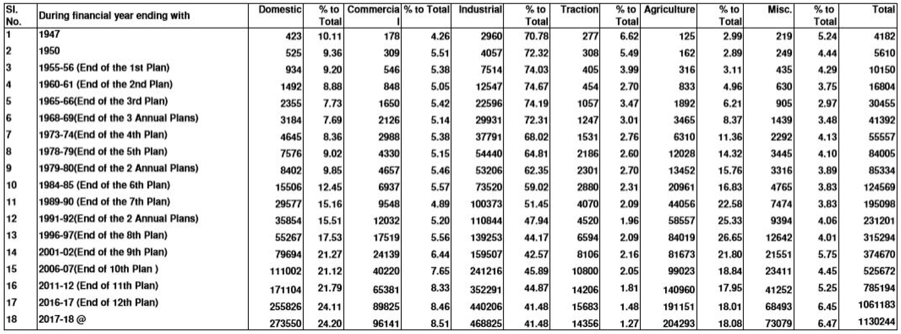
After the independence of the country, that is, in 1947 the TEC is observed to be 4182 GwH. At that time the domestic sector consumed around 10% of the overall and industrial sector consumed almost 71%, these two were the major players till the end of the 3rd plan. During the 1968–1969 that is, during the 3rd Annual plan the domestic sector experienced a dip compared to that of the agriculture sector and the Industrial and agriculture sector were found to be the major consumers till the end of the 9th plan that is, 2001–2002. During that point of time industrial sector consumed around 43% and the agriculture sector engulfed 21.8% which is just short of domestic sector 21.27%. Again from the end of the 19th plan till the end of the 12th plan that is, from 2001–2002 to 2016–2017 the domestic sector again started consuming more compared to the agriculture sector which was found to be 24.11% compared to agriculture’s 18.01%. Nevertheless the Industries have always been the major consumer since independence till date even though a decreasing trend is noticed overall. The traction sector in India has always followed a decreasing trend apart from a few periods which has also shown only a feeble increase. The Miscellaneous sector (others) has increased lately to 6.45% since independence compared to its 5.24% even though it is not a key consumer. This is an overview of the sector wise total energy consumption for India since 1947 as demonstrated in Figure 1.
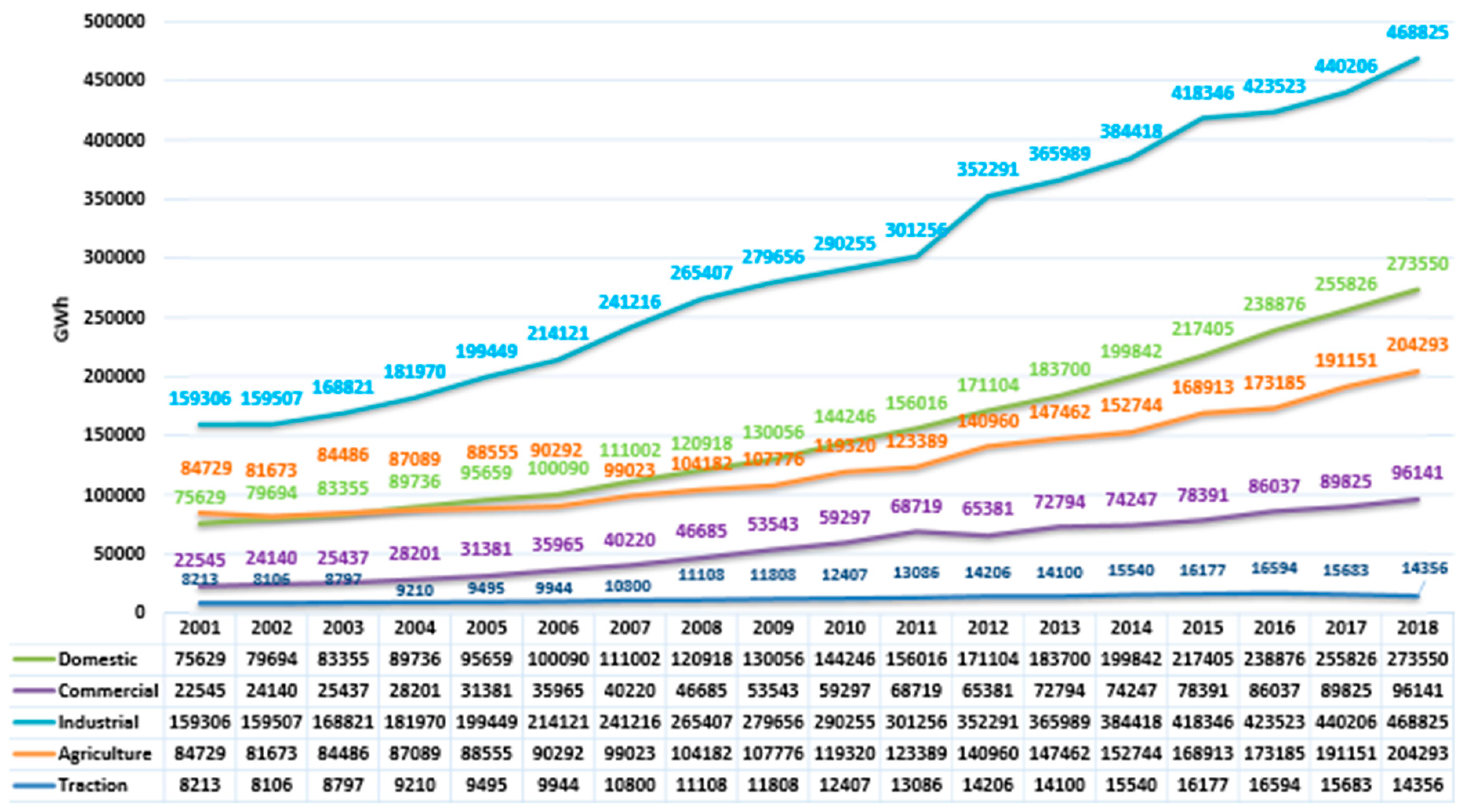
The graphical representation of the Domestic, Commercial, Industrial, Agricultural and Traction sectors for the period 2000–2018 has been shown in Figure 2. The value for the year 2018 is an estimated value compared to all the other values. The industrial sector has seen a steep increase since the start of the century which usually will be the case for any country. And all the other sectors have shown a gradual increase. The agriculture and the domestic categories have shown some fluctuations whereas the other sectors have shown a steady increase.
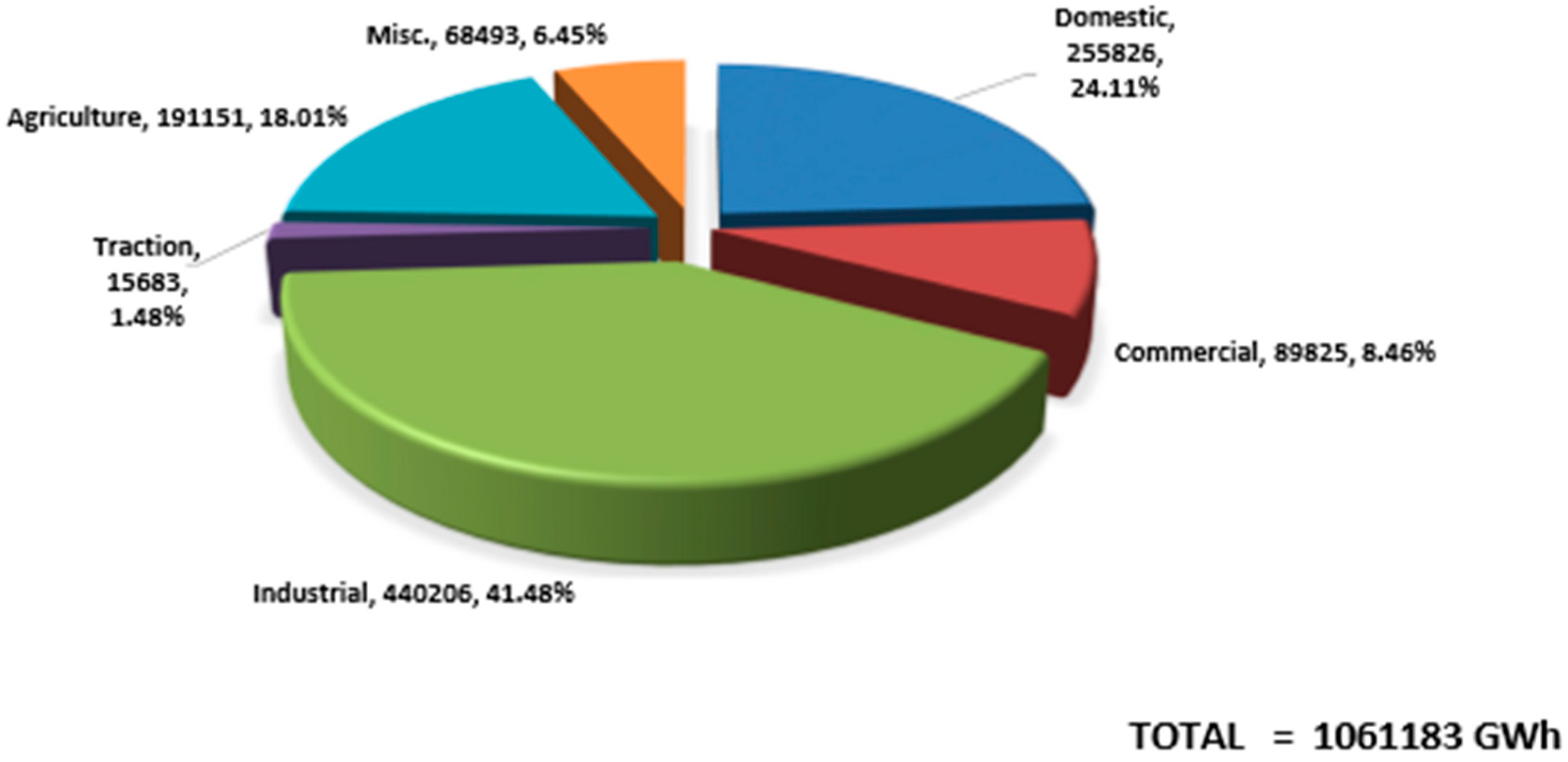
By the end of India’s 12th plan the split among all the sectors is shown above in Figure 3. The domestic and the agriculture which were going hand to hand, few decades earlier were found to show a visible contrast of over 6% between them. The industrial sector’s consumption over the years has decreased considerably even though it happened to be the vital consumer of all the sectors. And the same trend is expected to continue over the years which might transform India from being an Agriculture based economy.
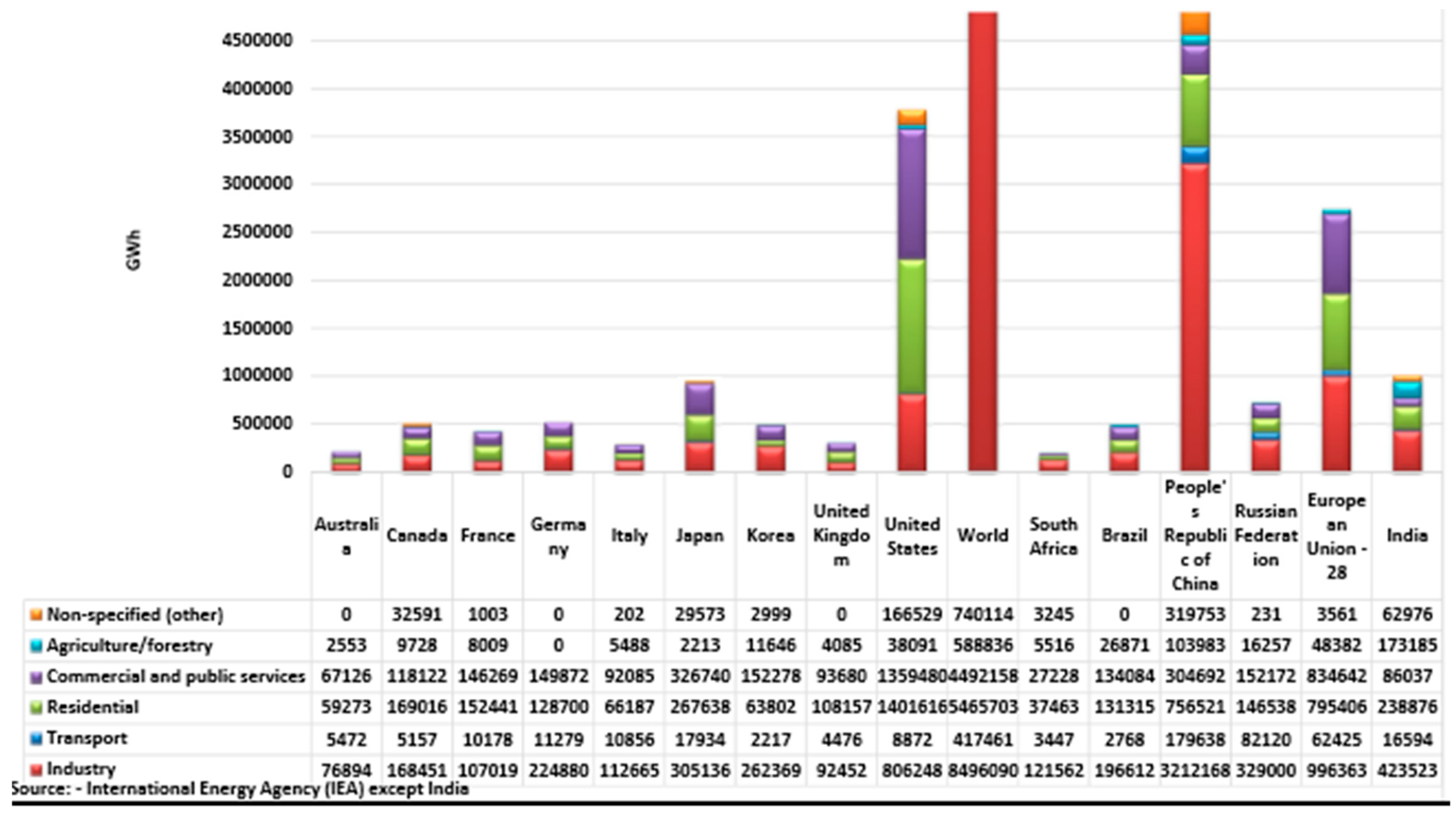
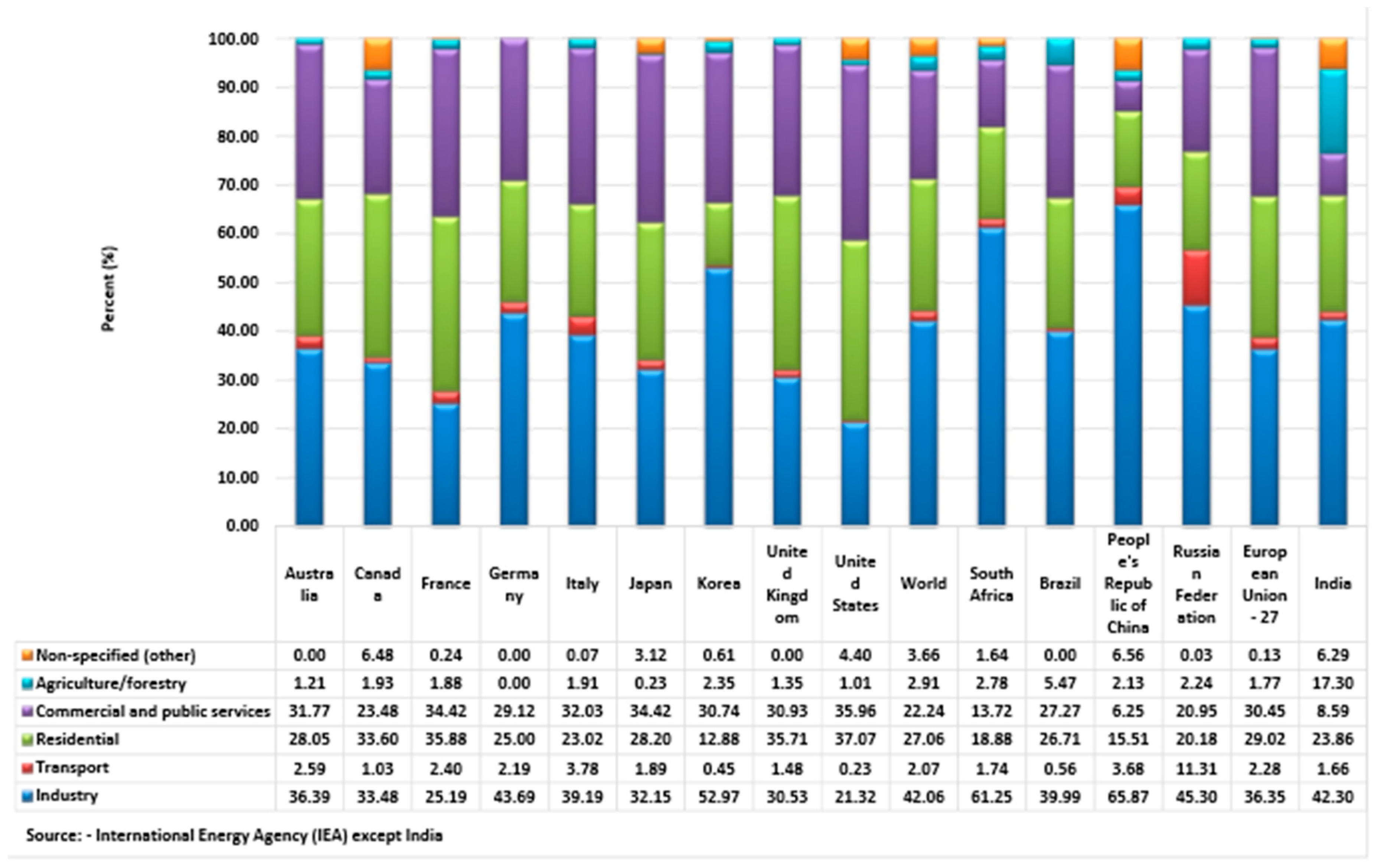
The category wise electricity consumption of India compared to other developed and developing countries are analysedin Figure 4 and Figure 5, along with the International Energy Agency’s report for the year 2015. India falls short of China and the US in terms of GWh in almost all the sectors except the agriculture sector. When compared to the European Union, India consumes electricity more in the agriculture sector and the others sector which is quite evident, since India is a tropical country and is agriculture based. India consumes 173,185 GWh of electricity which is higher than China’s 103,983 GWh which comes next. In the commercial sector US is the major electricity consumer, it tops the list with 1,359,480 GWh. US consumes 1,401,616 GWh in the residential sector which is almost the consumption of the Chinese republic’s 756,521 GWh and European Union’s 795,406 GWh combined, in spite of world’s highly populous nations such as China and India. In the transport category China’s 179,638 GWh electricity consumption stands out way ahead of the Russian federation’s 82,120 GWh, which is the second largest consumer. China is also the top consumer in the industrial sector in terms of electricity which is 32,121,168 GWh which is more than 26% of the whole world.
Energy Statistics brings out energy indicators meant for the practice of policy framers and for wide-ranging coverage. Indicators participate in a critical job by transforming the data to useful information for the plan makers and also aid in the process of making decisions. List of indicators identification depends upon various factors such as lucidity, technical validity, strength, sensitivity and the degree to which they are gelled to each other. No single factor can determine everything since each indicator needs different set of data. GDP is the country’s broadest quantitative gauge of total economic activity. In specific GDP tells us the financial value of all the goods and services manufactured within the country’s borders over a time span [34]. The data in the study has been gathered from the respective ministries of the Government of India (GoI). Energy intensity’s value has dipped over the latest ten years which might be ascribed to the quicker increase of GDP than the energy need.
3. Results
3.1. Linear Regression
In order to predict the influencing variable on Total Electricity Consumption (TEC) for India, Linear Regression is used initially. GDP, Population and GDP per Capita are taken as the input variables which are used one by one in linear regression to predict TEC.
The distance between the actual value and the mean is calculated and also the distance between the estimated line and its mean is calculated in the regression line. The comparison between the two values that is, the difference between the actual and mean and the difference between the estimated and the mean gives the R2 value.
1 − R2 = {SSR/SST}
SSR refers to the residual sum of squares and SST refers to the total sum of squares.
The standard error of the estimate is the distance between the estimated and the actual value. The constant value is actually the ‘y’ intercept of the line. The independent value is the slope of the regression line; since the line is linear the slope is also constant. The significance is the actual ‘p’ values.
where σ refers to the standard deviation, n refers to the sample size.
Standard Error (√n) = σ
3.1.1. Population
As depicted in Table 1, the constant value is −591,193.3447. The independent value that is, the slope of the regression line is 959,469.219; since the line is linear the slope is also constant. The regression equation usually frames a prediction and the precision of the prediction is calculated by means of the standard error. It also measures the scatter or dispersion of the observed values around the regression line.
Y = 959,469.219X − 591,193.347 is the regression equation.
3.1.2. GDP
As illustrated in Table 2, the constant value is 53,096.385. The independent value that is, the slope of the regression line is 417,965.826; since the line is linear the slope is also constant.
Y = 417,965.826X − 53,096.385 is the regression equation.
3.1.3. GDP per Capita
The constant value is −2457.344. The independent value that is, the slope of the regression line is 959,469.511; since the line is linear the slope is also constant as in Table 3.
Y = 546.511X − 2457.344 is the regression equation.
When we forecast Total Electricity Consumption (TEC) using three variables, the GDP plays an important role and it predicts better the Total Electricity Consumption than the GDP per Capita and the population. The R2 value for GDP and TEC is 0.957 whereas between GDP per capita and TEC it is only 0.951. When compared with Population and TEC it is even as lower as 0.845. Hence it is concluded that GDP foresees TEC better. The lowest std. error, 46,784.201 of all the three is also with the GDP.
3.2. Multiple Linear Regression
To forecast the TEC of electricity for 2030, multiple linear regression method is used now, taking in account the yearly GDP per capita, GDP and historical population data, as in the case of Turkey. During most of the situations, multiple independent variables might be used to predict the significance of a dependent variable for which we use multiple regression. In multiple regression, GDP and Population are taken simultaneously as the predicting variables. Multiple variable regression analysis establishes a relationship between a dependent variable (in this work Total Energy Consumption (TEC)) and two or even more than two independent variables that is, the predictors, population and GDPutilized an application technique for yearly consumption forecasting algorithm on the smart new intelligent electronic devices using multiple regression method which is put into practice in addition to recursive least square.
TEC = (332,023.240) Population + (302,638.253) GDP − 185,039.015is the regression equation from Table 4.
With one independent variable of population the R2 is 0.845 and with that of GDP it is 0.957, whereas with two independent variables GDP and population combined, in multiple linear regression the R2 increases to 0.986. The standard error of 46,784.201 with one variable, GDP drops to 27,442.309 with two variables. Lower is better. The GDP’s standard error is almost less than half of the population’s error. So GDP is again the better predictor in terms of Linear Multiple Regression.
3.3. Correlation Analysis
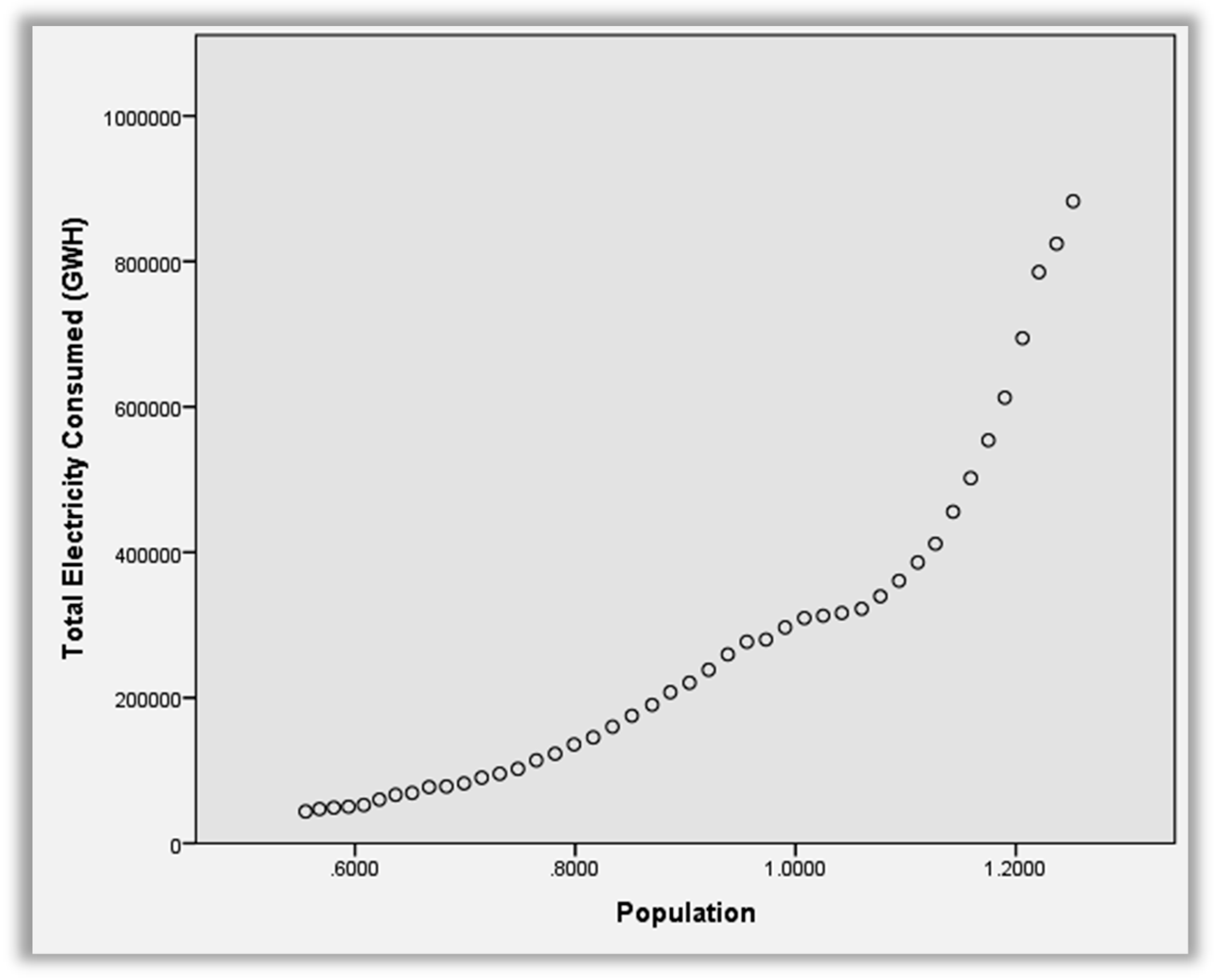
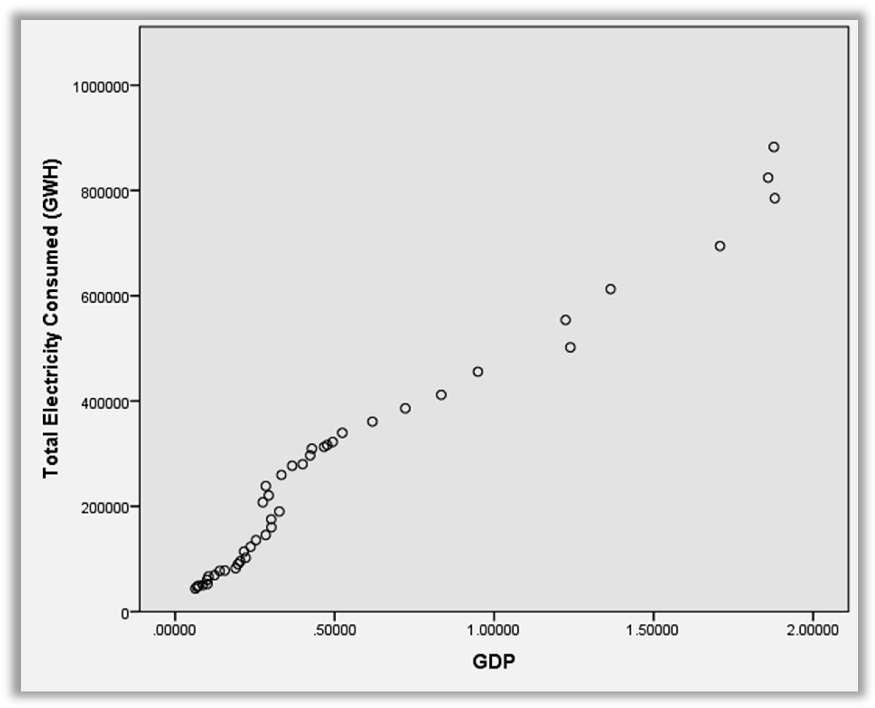
Almost all the independent variables exhibit a higher degree of correlation against the dependent variables, the analysis of correlation from Table 5 illustrates that there is positive high correlation between population and TEC. The Pearson correlation coefficient is found to be 0.919. From Figure 6, Figure 7 and Figure 8, the analysis of correlation between GDP and TEC proves that there is a very high positive correlation. The Pearson Correlation Coefficient is found to be 0.978Whereas the correlation between GDP per capita and TEC demonstrates that there is a positive comparatively low correlation between GDP and TEC. The Coefficient is found to be 0.975.
3.4. Simple Exponential Smoothing
If the time series vary about base level, simple exponential smoothing might be bring into play to find good estimates or upcoming value of the same series. To depict this phenomenon, let At the smoothed average of a time series. Subsequent to observing xt, At is the anticipate for the value of the time series during any upcoming period.
- At = smoothed average at the end of the epoch
- t = ft,
- k = for the forecast period (t + k) at the end of the epoch t.
Choose α so that it minimizes the MAD.
The key in equation in simple exponential smoothing is that
At = αxt + (1 − α) At − 1
In the Equation (1), α will be the smoothing constant that suit 0< α>1. To start the forecasting process, we have got to set a value for A0 before surveying x1. Typically, we let A0 be the experiential value for the period right away prior the first period. As among moving-average forecasts, we let ft,k be the estimate for xt + k ready at the final period t. Then
At = ft,k
Pretentious that we attempt to forecast one period ahead, the error for forecasting xt is
Et = xt − ft − 1,1 = xt − At − 1
The smoothing constant value considered for the analysis is α = 0.3, 0.4 and 0.5.
The TEC for 2015 was found to be 746,882 MW when α = 0.3 and 793,765 MW when α = 0.4 and 823,941.3 MW when α = 0.5.
3.4.1. Time Series Modeler—Expert Model (Sector Wise)
In the expert time series modeler it automatically assigns the model best suited based on the system’s expertise. For the industrial, agricultural and domestic sectors it has assigned Brown’s model and it is found to be the appropriate model. For the commercial, traction and others’ sector, the expert model has assigned ARIMA (0,1,0) model; ARIMA (2,1,0) model and ARIMA (0,1,0) respectively, automatically as the appropriate models as in Table 6. The respective degrees of freedom and other parameters are shown in Table 7.
3.4.2. Holt’s Model-Exponential Smoothing with Trend
Several models such as Brown’s model, Holt’s model, Expert model and damped trend model were analysed. And the analysis of the Holt’s model is shown in the Table 8.
3.4.3. Time Series Modeler (Exponential Smoothing-Brown)
The analysis of the Brown model is shown in the Table 9.
3.4.4. Time series modeler (Exponential Smoothing—Damped Trend)
The TEC for the years 2019, 2024 and 2030 were forecasted to be 1,162,453 MW, 1,442,410 MW and 1,778,358 MW respectively.
RMSE = √{Σ (Yactual − Yforecast)/N}
The Expert model selects different models on its own for different variables and produces the above mentioned forecast by means of a low root mean square error value, RMSE of 10,734.649 and a R2 value of 0.997 which is comparatively high. And the analysis of the Damped trend model is shown in the Table 10.
The forecasted values are shown in Table 11 for the above mentioned years.
3.5. Moving Average
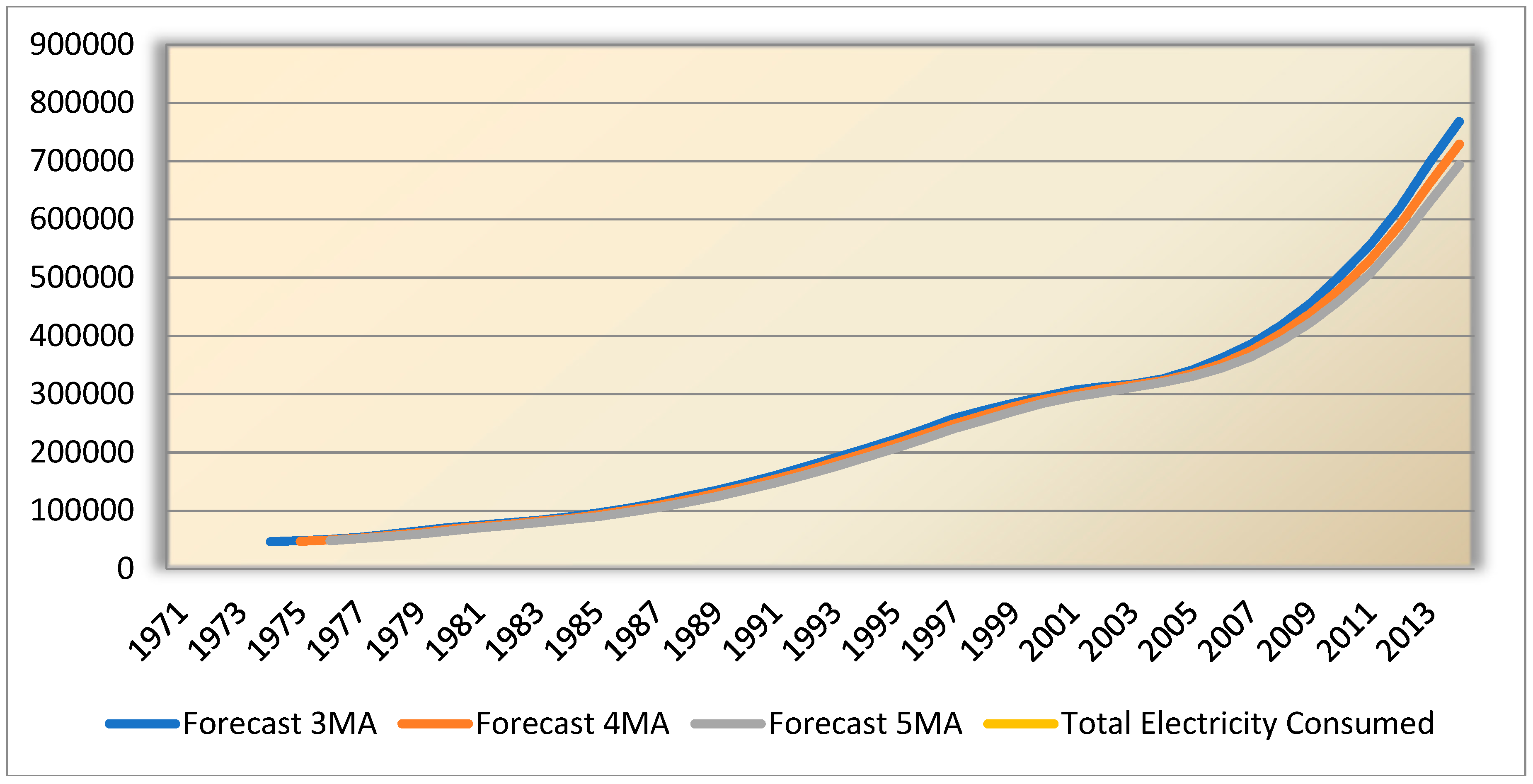
The three years’ four years’ and five years’ moving average for the time period of 1974–2014 is computed here and shown in Figure 9. The values were found to be 830,696, 796,620 and 759,825 MW respectively for the year 2014.
Moving average is one method which is very much suitable for short-term load forecasting, STLF. The forecast of the fourth year is the average of the first three years and so on.
3.6. Weighted Moving Average
The three years’ and four years’ weighted moving average for the time period 1971–2015 is calculated here. The values were found to be 786,587.1 and 765,421.5 MW respectively for the year 2015 in Figure 10.
For the three years weighted moving average the α value for the previous three years were 0.5, 0.3 and 0.2 respectively. The higher α value is allotted to the immediate month since it influences the outcome more than that of the previous values. For the four years weighted moving average the α value for the previous four years assigned were 0.4, 0.3, 0.2 and 0.1 respectively. It is made sure that the α values add up to 1.
3.7. Curve Estimation
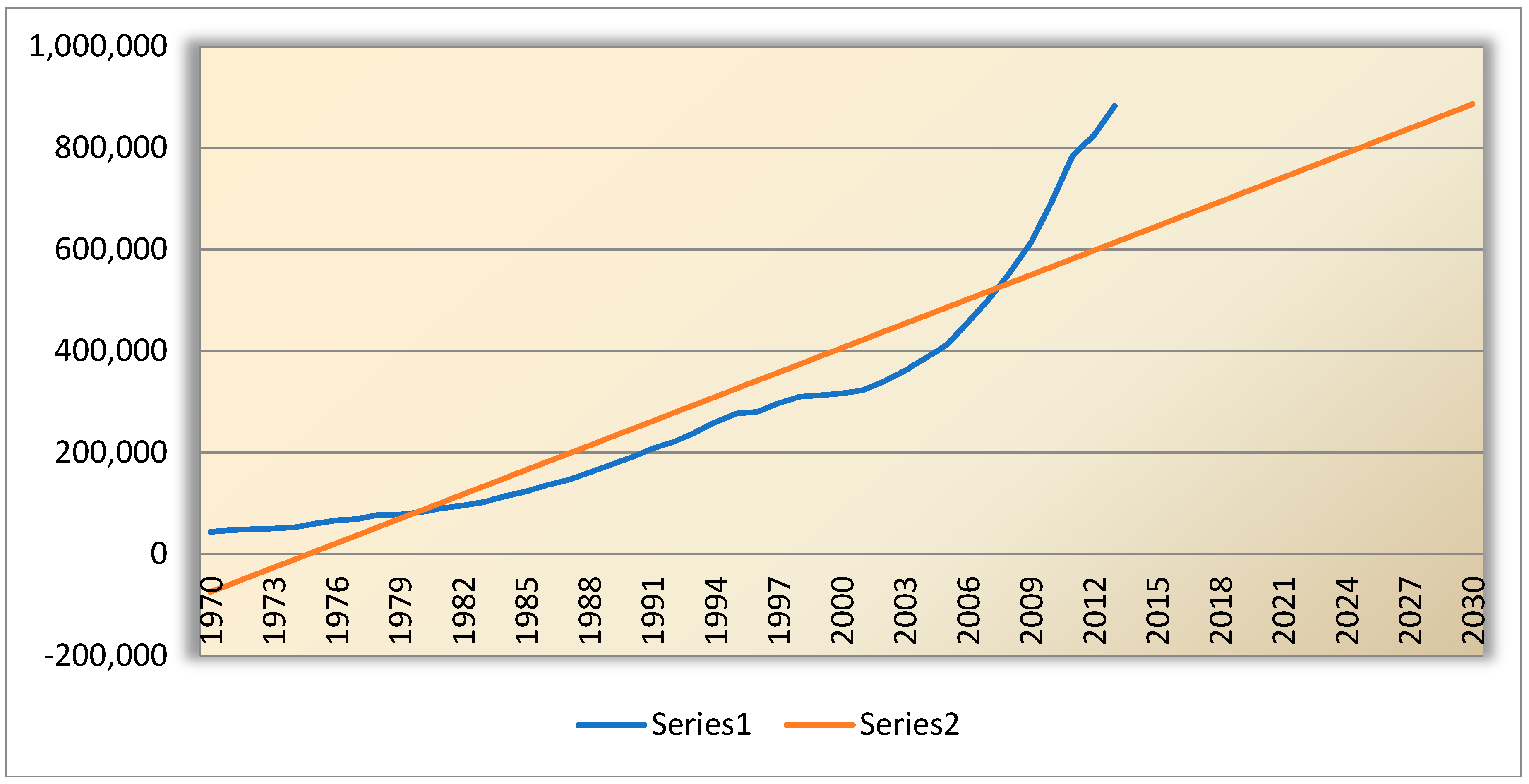
3.7.1. Linear Model
This Table 12 presents the regression coefficients and it is to be made a note of that, the correlation will be of negative value when the slope is negative. The following linear regression equation is determined by these coefficients.
y = −31,615,881.66 + 16,010.77x
Series 1 in the Figure 11 is the actual TEC and the series 2 is the linear forecast. The forecasted value for the linear curve fitting model for 2030 is 885,981.44 MW.
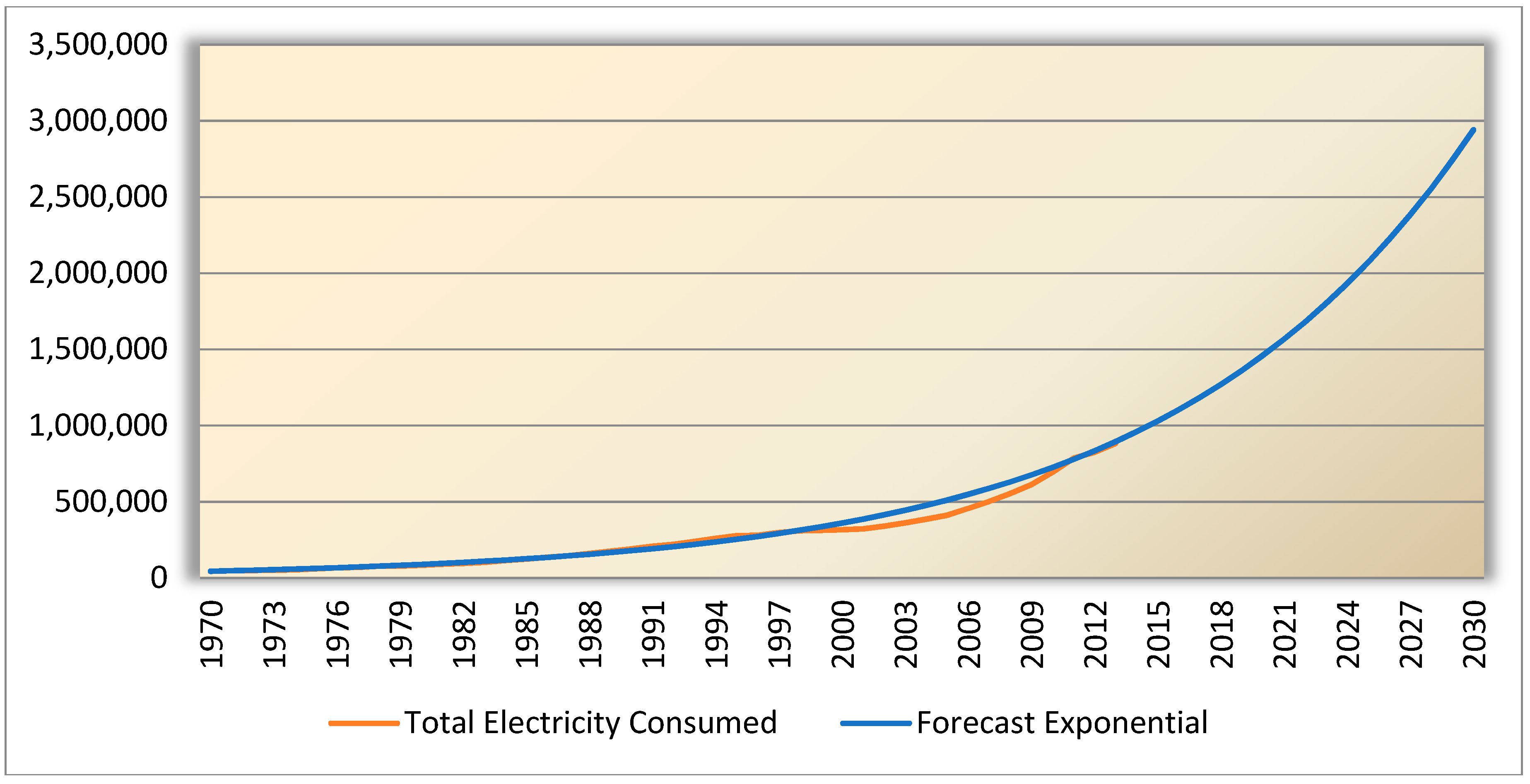
3.7.2. Compound/Exponential Model
The Table 13 represents the regression coefficients and it is to be taken into account that, the correlation will be in the negative side when the slope is of negative value. The following regression equation is made out of these coefficients.
y = 41,116.428e0.07x
The forecasted value for the compound curve fitting model for 2030 is 2,741,903.862 MW is plotted in Figure 12.
Similarly the regression equations for several other models shall also be interpreted.
4. Discussion
The measure of the adequacy of the fit is determined by the sample correlation (r) between the true value and responses got out of the fit. The sample correlation’s square is worked out readily out of the statistical package in the ANOVA and is termed the coefficient of determination (R2). The coefficient of determination is computed directly by estimating Pearson’s correlation ‘r’ between the predicted and the actual data. The coefficients of determination are generally expressed in terms of percentage. The value of R2 lies in between 0% and 100%. The nearer the value to the upper bound; the healthier will be the fit [35].
LEAP and Holt’s exponential smoothing method were also employed to estimate the electricity energy demand for 2030 in Maharashtra, India in that study. ANN, multiple regression approaches and ANOVA were used. It is evident from the analysis of variance in this article that the regression method is able to forecast the cutting forces with a higher accuracy [36] which supports the present study. An optimal renewable energy model, OREM for India was evolved for the year 2020–2021 to meet the increasing energy requirements [37]. An optimization model for various end-uses was formulated by determining the optimum allocation of renewable energy for 2020–2021, by considering the energy requirement of the commercial sector. This study revealed that the social acceptance of bio resources increased by 3% and solar PV utilizationdecreased by 65% [38].Various energy demand forecasting models were reviewed by [39] and found that traditional methods viz., time series regression, econometric analysis are extensively made use for demand side management whereas the TEC is calculated for 2030 in this paper. Regression analysis, linear model analysis and R2 correlation value was built by [40] for a curved vane demister which supports the using linear model analysis of the current study. The utilization of black box approach to forecast the TEC for India is supported by vast literature among which an optimal renewable energy model for India for 2020–2021 was presented by distributing renewable energy effectively to help the policy framers in marketing the renewable energy resources and to determine the optimized allotment of various non-conventional energy resources for various end-uses. In this study linear as well as multiple regression analysis proves GDP is again the better predictor in terms of Multiple linear regression. Therefore, a sensible energy forecast is needed for the policy framers while taking decision for the future. Thus, the policy framers need to take this boost in energy usage in mind. It is also recommended that the other energy forecasting techniques shall also be used to testify the outcome and also energy prediction shall be recurrently done as the circumstances are dynamic.
Some of the state of art work in the same research area is discussed here
- According to National Energy Map for India: Technology Vision 2030, India’s electricity consumption will become fourfold from about 1.1 trillion units to 4 trillion units by2030.Brookings Institution India Centre, in 2013, estimated that the shoot up in global energy consumption is attributed mainly due to India and China [41].
- Asia-Pacific territory lonely contributes to 79% of the hike in international liquids use, which rises from 1281.7 Million tons of oil equivalent in 2010 to 1859.3 Million tons of oil equivalent in 2030. The per capita energy utilization in 2030 for India is expected to rise from 19.58 million Btu to 29.84 million Btu [42].
- The former Coal and power minister of India, Mr. Piyush Goyal stated in May, 2016 that a possible 10% jump is expected in the annual electricity growth for the next 15 or 16 years [43].
- Sugandha Chauhan (2017) studied electricity demand and reported that it will increase from 1115 BU in 2015–2016 to 1692 BU in 2022, 2509 BU in 2027 and 3175 BU in 2030 reflecting the higher end of the demand for electricity [44].
- Iniyan et al. 2000. proposed a model that allocates the renewable energy distribution pattern for the year 2020–2021 for India [45].
5. Conclusions
This work presents the analysis of available data and the predicted one regarding what will be the Total Electricity Consumption (TEC) of India for the year 2030 using various black box based approaches. The forecasting of total electricity consumption for the year 2030–2031 for India is found to be 1,834,349MW while doing so the forecast for 2017 was compared with the actual data given by Energy statistics, GOI which sits close to the forecasted data. And the expert model is forecasted to be the best fit that suits the prediction since the R2 value is 0.997 which is comparatively high. Obtained results show that this model is of a high precision. The advantages of the model are that it can be computed easily with simple statistical software and available in almost every recent statistical package. Accessibility is not an obstacle and the analysis shall be performed with a device of minimal configuration. The time taken for running the model is very minimal which is a mere 00:00:00.06 s (processor time). The disadvantage of the model is that it selects the best suitable model on its own. The limitation of the work is that we could not apply the popular methodologies of black box approaches such as Decision Trees, ANN, SVM. There are several other variables such as imports, exports, villages electrified, pump sets energized and so forth, which has a futuristic scope for further extensive studies. Energy forecasting can be taken up to the next level, for example, for Asia-Pacific territory. As the need for energy consumption is constantly increasing in manifolds, it is assumed that the findings and forecasts given in this article would be of use to the policy makers and energy strategists to evolve future scenarios for the Indian electricity consumption which should focus greatly in further increasing the overall share of renewable energy resources compared to the conventional sources of the installed capacity as well as in the consumption pattern. The future research may be done considering more input variables such as the quantum of CO2 emission, GNP per capita, consumer price index, power consumption per capita, wholesale price index, imports, gross domestic savings, exports and so forth. Other methodologies such as computational intelligence forecasts, beyond point forecasts, combined forecasts may also be applied in short term load forecasting of the electrical energy demand.
Author Contributions
Conceptualization, H.R. and I.S.; Methodology, H.R.; Software, H.R.; Validation, H.R.; Formal Analysis, H.R. and I.S.; Investigation, I.S. and J.B.A.; Resources, H.R. and J.B.A.; Data Curation, H.R.; Writing-Original Draft Preparation, H.R.; Writing-Review & Editing, I.S. and J.B.A.; Supervision, I.S. H.R., IniyanSelvarasanand J.B.A. have added inputs in developing strategies for total energy consumption forecasting and the collection of the data set was taken care by H.R. All the authors were involved in drafting and revising the manuscript.
Funding
This research received no external funding.
Acknowledgments
The corresponding author first thanks the Al Mighty. He next expresses his gratitude to his parents who help him greatly to carry out his research work. He whole heartedly thanks his research supervisor for his invaluable guidance. The authors thank K. Padmanathan, who made available some of the data. He also thanks the authorities and faculty in Department of Mechanical engineering, Anna University, Chennai.
Conflicts of Interest
The authors declare no conflict of interest.
References
- Central Electricity Authority. Available online: www.cea.nic.in (accessed on 15 October 2018).
- Kalyani, K.A.; Pandey, K.K. Waste to Energy Status in India: A Short Review. Renew. Sustain. Energy Rev. 2014, 31, 113–120. [Google Scholar] [CrossRef]
- Alagh, Y.K. The Food, Water and Energy, Inter Linkages for Sustainable Development in India. South Asian Surv. 2010, 17, 159–178. [Google Scholar] [CrossRef]
- Taylor, J.W. Triple seasonal methods for short-term electricity demand forecasting. Eur. J. Oper. Res. 2010, 204, 139–152. [Google Scholar] [CrossRef] [Green Version]
- Taylor, J.W.; McSharry, P.E. Short-Term Load Forecasting Methods: An Evaluation Based on European Data. IEEE Trans. Power Syst. 2008, 22, 2213–2219. [Google Scholar] [CrossRef]
- Park, D.C.; El-Sharkawi, M.A.; Marks, R.J.; Atlas, L.E.; Damborg, M.J. Electric Load Forecasting Using an Artificial Neural Network. IEEE Trans. Power Syst. 1991, 6, 442–449. [Google Scholar] [CrossRef]
- Mohamed, Z.; Bodger, P. Forecasting electricity consumption in New Zealand using economic and demographic variables. Energy 2005, 30, 1833–1843. [Google Scholar] [CrossRef] [Green Version]
- Haida, T.; Muto, S. Regression based peak load forecasting using a transformation technique. IEEE Trans. Power Syst. 1994, 9, 1788–1794. [Google Scholar] [CrossRef]
- Mirasgedis, S.; Safaridis, Y.; Georgopoulou, E.; Lalas, D.P.; Moschovits, M.; Karagiannis, F.; Papakonstantinou, D. Models for mid-term electricity demand forecasting incorporating weather influences. Energy 2006, 31, 208–227. [Google Scholar] [CrossRef]
- Da, X.; Jiangyan, Y.; Jilai, Y. The physical series algorithm of mid-long term load forecasting of power systems. Electr. Power Syst. Res. 2000, 53, 31–37. [Google Scholar] [CrossRef]
- Muis, Z.A.; Hashim, H.; Manan, Z.A.; Taha, F.M.; Douglas, P.L. Optimal planning of renewable energy—Integrated electricity generation schemes with CO2 reduction target. Renew. Energy 2010, 35, 2562–2570. [Google Scholar] [CrossRef]
- Kale, R.V.; Pohekar, S.D. Electricity demand and supply scenarios for Maharashtra (India) for 2030: An application of long range energy alternatives planning. Energy Policy 2014, 72, 1–13. [Google Scholar] [CrossRef]
- Messner, S.; Golodnikov, A.; Gritsevskii, A. A Stochastic version of the dynamic linear programming model, MESSAGE III. Energy 1996, 21, 775–784. [Google Scholar] [CrossRef]
- Tardioli, G.; Kerrigan, R.; Oates, M.; O’Donnell, J.; Finn, D. Data driven approaches for prediction of building energy consumption at urban level. Energy Procedia 2015, 78, 3378–3383. [Google Scholar] [CrossRef]
- Choi, M.S.; Xiang, L.; Lee, S.J.; Kim, T.W. An Innovative Application Method of Monthly Load Forecasting for Smart IEDs. J. Electr. Eng. Technol. 2013, 8, 984–990. [Google Scholar] [CrossRef] [Green Version]
- Yalcinoz, T.; Eminoglu, U. Short term and medium term power distribution load forecasting by neural networks. Energy Convers. Manag. 2005, 46, 1393–1405. [Google Scholar] [CrossRef]
- Chen, G.J.; Li, K.K.; Chung, T.S.; Sun, H.B.; Tang, G.Q. Application of an innovative combined forecasting method in power system load forecasting. Electr. Power Syst. Res. 2001, 59, 131–137. [Google Scholar] [CrossRef]
- Mestekemper, T.; Kauermann, G.; Smith, M.S. A comparison of periodic autoregressive and dynamic factor models in intraday energy demand forecasting. Int. J. Forecast. 2013, 29, 1–12. [Google Scholar] [CrossRef]
- Tsekouras, G.J.; Dialynas, E.N.; Hatziargyriou, N.D.; Kavatza, S. A non-linear multivariable regression model for midterm energy forecasting of power systems. Electr. Power Syst. Res. 2007, 77, 1560–1568. [Google Scholar] [CrossRef]
- Persaud, J.; Kumar, U. An eclectic approach in energy forecasting: A case of Natural Resources Canada’s oil and gas outlook. Energy Policy 2001, 29, 303–313. [Google Scholar] [CrossRef]
- Edigera, V.S.; Akarb, S. ARIMA forecasting of primary energy demand by fuel in Turkey. Energy Policy 2007, 35, 1701–1708. [Google Scholar] [CrossRef]
- Xie, N.-M.; Yuan, C.-Q.; Yang, Y.-J. Forecasting China’s energy demand and self-sufficiency rate by grey forecasting model and Markov model. Elect. Power Energy Syst. 2015, 66, 1–8. [Google Scholar] [CrossRef]
- Bassam, M.; Al-Foul, A. Forecasting Energy Demand in Jordan Using Artificial Neural Networks. Top. Middle East. Afr. Econ. 2012, 14, 473. [Google Scholar]
- Kankal, M.; Akpınar, A.; Komurcu, M.I.; Ozsahin, T.S. Modeling and forecasting of Turkey’s energy consumption using socio-economic and demographic variables. Appl. Energy 2011, 88, 1927–1939. [Google Scholar] [CrossRef]
- Hyndman, R.J.; Fan, S. Density Forecasting for Long-Term-Peak Electricity Demand. IEEE Trans. Power Syst. 2010, 25, 1142–1153. [Google Scholar] [CrossRef]
- Pławiak, P. Novel Genetic Ensembles of Classifiers Applied to Myocardium Dysfunction Recognition Based on ECG Signals. Swarm Evol.Comput. 2018, 39, 192–208. [Google Scholar] [CrossRef]
- Pławiak, P.; Rzecki, K. Approximation of Phenol Concentration using Computational Intelligence Methods Based on Signals from the Metal Oxide Sensor Array. IEEE Sens. J. 2015, 15, 1770–1783. [Google Scholar]
- Mallah, S.; Bansal, N.K. Allocation of energy resources for power generation in India: Business as usual and energy efficiency. Energy Policy 2010, 38, 1059–1066. [Google Scholar] [CrossRef]
- Li, C.; Ding, Z.; Zhao, D.; Yi, J.; Zhang, G. Building Energy Consumption Prediction: An Extreme Deep Learning Approach. Energies 2017, 10, 1–20. [Google Scholar] [CrossRef]
- Bianco, V.; Manca, O.; Nardini, S. Electricity consumption forecasting in Italy using linear regression models. Energy 2009, 34, 1413–1421. [Google Scholar] [CrossRef]
- Erdogdu, E. Electricity demand analysis using co-integration and ARIMA modeling: A case study of Turkey. Energy Policy 2007, 35, 1129–1146. [Google Scholar] [CrossRef]
- Gajowniczek, K.; Nafkha, R.; Ząbkowski, T. Electricity peak demand classification with artificial neural networks. Ann.Comput. Sci. Inf. Syst. 2017, 11, 307–315. [Google Scholar] [Green Version]
- Singh, S.; Yassine, A. Big Data Mining of Energy Time Series for Behavioral Analytics and Energy Consumption Forecasting. Energies 2018, 11, 452. [Google Scholar] [CrossRef]
- Energy Statistics 2018; Central Statistics Office, Ministry of Statistics and Programme Implementation, Government of India: New Delhi, India, 2018.
- Robert Mason, L.; Richard Gunst, F.; James Hess, L. Statistical Design and Analysis of Experiments; John Wiley & Sons Publication: New York, NY, USA, 2003. [Google Scholar]
- Hanief, M.; Wani, M.F.; Charoo, M.S. Modeling and prediction of cutting forces during the turning of red brass (C23000) using ANN and regression analysis. Eng. Sci. Technol. Int. J. 2017, 20, 1220–1226. [Google Scholar] [CrossRef]
- Iniyan, S.; Suganthi, L.; Jagadeesan, T.R.; Samuel, A.A. Reliability based socio economic optimal renewable energy model for India. Renew. Energy 2000, 19, 291–297. [Google Scholar] [CrossRef]
- Suganthi, L.; Williams, A. Renewable energy in India—A modelling study for 2020–2021. Energy Policy 2000, 28, 1095–1109. [Google Scholar] [CrossRef]
- Suganthi, L.; Samuel, A.A. Energy models for demand forecasting—A review. Renew. Sus. Energy Rev. 2012, 16, 1223–1240. [Google Scholar] [CrossRef]
- Venkatesan, G.; Kulasekharan, N.; Muthukumar, V.; Iniyan, S. Regression analysis of a curved vane demister with Taguchi based optimization. Desalination 2015, 370, 33–43. [Google Scholar] [CrossRef]
- TERI. National Energy Map for India: Technology Vision 2030: Summary for Policy-Makers; The Energy and Resources Institute TERI & Office of the Principal Scientific Adviser, Government of India: New Delhi, India, 2015.
- Gokarn, S.; Sajjanhar, A.; Sandhu, R.; Dubey, S. Energy 2030; Brookings Institution India Center: New Delhi, India, 2013. [Google Scholar]
- The Economic Times. Available online: https://economictimes.indiatimes.com/industry/energy/power/indias-electricity-consumption-to-touch-4-trillion-units-by-2030/articleshow/52221341.cms (accessed on 21 November 2018).
- Chauhan, S.; Shekhar, S.; D’Souza, S.; Gopal, I. Transitions in Indian Electricity Sector 2017–2030; The Energy and Resources Institute TERI: New Delhi, India, 2017. [Google Scholar]
- Iniyan, S.; Sumathy, K. An optimal renewable energy model for various end-uses. Energy 2000, 25, 563–575. [Google Scholar] [CrossRef]
Figure 1.
Category wise TEC growth in India (1947–2018).

Figure 2.
Sector wise Energy Consumption since the Century (2000–2018).

Figure 3.
India’s Electricity Consumption by the end of 12th Plan (31 March 2017).

Figure 4.
Category-wise Electricity Consumption across various countries (2015).

Figure 5.
Category-wise % Shares in Electricity Consumption across various countries (2015).

Figure 6.
Plot between Population and TEC.

Figure 7.
Plot between GDP and TEC.

Figure 8.
Plot between GDP per Capita and TEC.

Figure 9.
Chart for moving average method (1971–2014).

Figure 10.
Chart for Weighted moving average method (1971–2015).

Figure 11.
Chart for Linear method (1971–2030).

Figure 12.
Chart for Exponential method (1971–2030).


Table 1.
Summary of the model with Population as the variable.
| Ind. Variable | R Square | Std. Error | Constant | Slope | Significance |
|---|---|---|---|---|---|
| Population | 0.845 | 89,127.342 | −591,193.347 | 959,469.219 | 0.000 |
Table 2.
Summary of the model with GDP as the variable.
| Ind. Variable | R Square | Std. Error | Constant | Slope | Significance |
|---|---|---|---|---|---|
| GDP | 0.957 | 46,784.201 | 53,096.385 | 417,965.826 | 0.000 |
Table 3.
Summary of the model with GDP per capita as the variable.
| Ind. Variable | R Square | Std. Error | Constant | Slope | Significance |
|---|---|---|---|---|---|
| GDP/Capita | 0.951 | 50,234.297 | −2457.344 | 546.511 | 0.000 |
Table 4.
Summary of the model with both Population and GDP as the variable.
| Ind. Variable | R Square | Std. Error | Constant | Slope | Significance |
|---|---|---|---|---|---|
| Population | 0.986 | 27,442.309 | −185,039.015 | 332,023.240 | 0.000 |
| GDP | 0.986 | 27,442.309 | −185,039.015 | 302,638.253 | 0.000 |
Table 5.
Correlation Matrix.
| Variables | TEC | Outcome | Direction |
|---|---|---|---|
| Population | 0.919 | High correlation | Positive |
| GDP | 0.978 | Very high correlation | Positive |
| GDP/Capita | 0.975 | High correlation | Positive |
Table 6.
Summary of Expert model.
| Model ID | Model Type |
|---|---|
| Industry | Brown |
| Agriculture | Brown |
| Domestic | Brown |
| Commercial | ARIMA (0,1,0) |
| Traction Railways | ARIMA (2,1,0) |
| Others | ARIMA (0,1,0) |
Table 7.
Summary of the model.
| Model | Statistics | Ljung-Box | No. of Outliers | ||
|---|---|---|---|---|---|
| Stationary R2 | Statistics | DF | Sig. | ||
| Industry | 0.281 | 3.802 | 17 | 1.00 | 0 |
| Agriculture | 0.080 | 49.040 | 17 | 0.000 | 0 |
| Domestic | 0.432 | 6.242 | 17 | 0.991 | 0 |
| Commercial | 1.102 × 10⁻¹⁵ | 10.125 | 18 | 0.928 | 0 |
| Traction/Railways | 0.331 | 15.057 | 17 | 591 | 0 |
| Others | 5.310 × 10⁻¹⁶ | 20.114 | 18 | 0.326 | 0 |
Table 8.
Summary of Holt’s model.
| Model | Statistics | Ljung-Box | No. of Outliers | ||
|---|---|---|---|---|---|
| Stationary R2 | Statistics | DF | Sig. | ||
| Industry | 0.291 | 2.371 | 16 | 1.00 | 0 |
| Agriculture | 0.103 | 43.582 | 16 | 0.000 | 0 |
| Domestic | 0.447 | 6.536 | 16 | 0.981 | 0 |
| Commercial | 0.422 | 3.726 | 16 | 0.999 | 0 |
| Traction/Railways | 0.394 | 35.017 | 16 | 0.004 | 0 |
| Others | 0.434 | 19.379 | 16 | 0.250 | 0 |
| TEC | 0.069 | 14.250 | 16 | 0.580 | 0 |
Table 9.
Summary of Brown model.
| Model | Statistics | Ljung-Box | No. of Outliers | ||
|---|---|---|---|---|---|
| Stationary R2 | Statistics | DF | Sig. | ||
| Industry | 0.281 | 3.802 | 17 | 1.00 | 0 |
| Agriculture | 0.80 | 49.040 | 17 | 0.000 | 0 |
| Domestic | 0.432 | 6.242 | 17 | 0.991 | 0 |
| Commercial | 0.421 | 3.999 | 17 | 0.999 | 0 |
| Traction/Railways | 0.393 | 33.210 | 17 | 0.011 | 0 |
| Others | 0.411 | 23.559 | 17 | 0.132 | 0 |
| TEC | 0.067 | 14.569 | 17 | 0.627 | 0 |
Table 10.
Summary of Damped trend model.
| Model | Statistics | Ljung-Box | No. of Outliers | ||
|---|---|---|---|---|---|
| Stationary R2 | Statistics | DF | Sig. | ||
| Industry | 0.392 | 2.365 | 15 | 1.00 | 0.392 |
| Agriculture | 0.337 | 44.861 | 15 | 0.000 | 0.337 |
| Domestic | 0.570 | 6.543 | 15 | 0.969 | 0 |
| Commercial | 0.467 | 3.720 | 15 | 0.999 | 0 |
| Traction/Railways | 0.114 | 34.625 | 15 | 0.003 | 0 |
| Others | 0.062 | 19.223 | 15 | 0.204 | 0 |
| TEC | 0.760 | 14.245 | 15 | 0.507 | 0 |
Table 11.
Summary of the results and Time line forecasted values for 2030.
| Sector | Model | 2019 | 2024 | 2030 |
|---|---|---|---|---|
| Industry | Brown | 538,089 | 686,457 | 864,498 |
| Agriculture | Brown | 208,891 | 258,836 | 318,770 |
| Domestic | Brown | 259,381 | 321,054 | 395,062 |
| Commercial | ARIMA | 115,130 | 172,213 | 279,201 |
| Traction/Railways | ARIMA | 20,554 | 26,906 | 465,523 |
| Others | ARIMA | 68,072 | 100,343 | 37,404 |
| TEC | Brown | 1,162,453 | 1,442,410 | 1,778,358 |
Table 12.
Summary of Linear model.
| Equation | Summary of the Model | Parameter Estimates | |||
|---|---|---|---|---|---|
| R2 | df1 | df2 | Sig. | Constant | |
| Linear | 0.844 | 1 | 42 | 0.000 | −31,615,881.66 |
Table 13.
Summary of the model.
| Equation | Summary of the Model | Parameter Estimates | |||
|---|---|---|---|---|---|
| R2 | df1 | df2 | Sig. | Constant | |
| Comp./Exp. | 0.991 | 1 | 42 | 0.000 | 41,116.428 |
© 2018 by the authors. Licensee MDPI, Basel, Switzerland. This article is an open access article distributed under the terms and conditions of the Creative Commons Attribution (CC BY) license (http://creativecommons.org/licenses/by/4.0/).
Share and Cite
MDPI and ACS Style
Rahman, H.; Selvarasan, I.; Begum A, J. Short-Term Forecasting of Total Energy Consumption for India-A Black Box Based Approach. Energies 2018, 11, 3442. https://doi.org/10.3390/en11123442
AMA Style
Rahman H, Selvarasan I, Begum A J. Short-Term Forecasting of Total Energy Consumption for India-A Black Box Based Approach. Energies. 2018; 11(12):3442. https://doi.org/10.3390/en11123442
Chicago/Turabian StyleRahman, Habeebur, Iniyan Selvarasan, and Jahitha Begum A. 2018. "Short-Term Forecasting of Total Energy Consumption for India-A Black Box Based Approach" Energies 11, no. 12: 3442. https://doi.org/10.3390/en11123442
Note that from the first issue of 2016, this journal uses article numbers instead of page numbers. See further details here.