Deep Learning Based on Multi-Decomposition for Short-Term Load Forecasting


Department of Electrical and Electronic Engineering, Yonsei University, Seoul 03722, Korea
*
Author to whom correspondence should be addressed.
Energies 2018, 11(12), 3433; https://doi.org/10.3390/en11123433
Submission received: 31 October 2018
/
Revised: 29 November 2018
/
Accepted: 3 December 2018
/
Published: 7 December 2018
(This article belongs to the Special Issue Short-Term Load Forecasting by Artificial Intelligent Technologies)
Abstract
:Load forecasting is a key issue for efficient real-time energy management in smart grids. To control the load using demand side management accurately, load forecasting should be predicted in the short term. With the advent of advanced measuring infrastructure, it is possible to measure energy consumption at sampling rates up to every 5 min and analyze the load profile of small-scale energy groups, such as individual buildings. This paper presents applications of deep learning using feature decomposition for improving the accuracy of load forecasting. The load profile is decomposed into a weekly load profile and then decomposed into intrinsic mode functions by variational mode decomposition to capture periodic features. Then, a long short-term memory network model is trained by three-dimensional input data with three-step regularization. Finally, the prediction results of all intrinsic mode functions are combined with advanced measuring infrastructure measured in the previous steps to determine an aggregated output for load forecasting. The results are validated by applications to real-world data from smart buildings, and the performance of the proposed approach is assessed by comparing the predicted results with those of conventional methods, nonlinear autoregressive networks with exogenous inputs, and long short-term memory network-based feature decomposition.
1. Introduction
Accurate load forecasting optimizes power loads, reducing costs and stabilizing electric power distribution. Load forecasting accuracy depends on the time series data of non-stationary and non-linearity characteristics. These characteristics are influenced by the prediction time scale and energy consumption scale. Depending on the prediction time scale, load forecasting is classified into four types.
Long-term load forecasting (LTLF) has a time scale of more than a year, medium-term load forecasting (MTLF) a time scale from one week to one year, and short-term load forecasting (STLF) a time scale from one hour to one week. System operators typically estimate demand by referring to load profiles from several hours ago. Ultra-short-term load forecasting (USTLF) is a key issue for smart grids, real-time demand side management (DSM), and energy transactions because energy trading in DSM requires precise load forecasting in the order of minutes, and profit is strongly related to forecast accuracy. Therefore, the USTLF time scale is from several minutes to one hour [1].
Conventional load forecasting methods use statistical models based on inherent characteristics of historical data. Previous STLF studies have proposed auto-regressive integrated moving average (ARIMA), Gaussian processing regression (GPR), support vector regression (SVR), and neural network models [2]. ARIMA is a common method for linear time series-based methods. GPR and SVR provide alternative methods to model time series loads, using external data such as weather data to consider non-linearity and non-stationarity. GPR is a supervised machine learning model based on statistical regression and a kernel function that refines variance and step length [3].
To reduce the nonlinearity of the time series data and to analyze their statistical characteristics, a seasonal analysis combined prediction method is used [4,5]. Recent research activities divide profiles into sub-profiles according to the load patterns of customers based on human factor, contract type, and region. After dividing the profiles into sub-profiles, a clustering algorithm is used for hierarchical classification [6,7,8,9].
To improve the accuracy of load forecasting using external data such as temperature, humidity, weather information, and electricity prices, a method has been proposed [10,11,12,13]. However, measuring such data is a challenging task for low-level distribution and small-scale loads. Furthermore, data processing and data storage of each piece of the dataset are required because the resolution of time-series data is different. Therefore, recent research trends use the technique of feature selection [14,15] or decomposing the load profile to extract the characteristics of the load using signal processing theory [16,17,18,19,20,21,22,23,24].
Wavelet decomposition with neural networks [1,16,17,18] has been employed to increase prediction accuracy. In [1], a wavelet algorithm dealt with the noise of the actual electrical load data, and load forecasting based on artificial neural networks (ANN) was proposed. Empirical mode decomposition (EMD) with machine learning has also been proposed for load forecasting, wind speed, or energy prices [19,20,21,22]. However, EMD lacks a mathematical definition and has weaknesses that diverge at end-points when decomposing the signal. To overcome the weakness of EMD, load forecasting studies using variational mode decomposition (VMD) have been proposed [22,23,24,25]. Existing regression methods with various decompositions, clustering algorithms, and probabilistic analyses have been investigated, as they can be used to identify load characteristics; however, they increase the dimension of the input [26,27,28]. Clustering and decomposition methods are applied in the pre-processing stage to improve the accuracy of the load prediction, and current state-of-art load forecasting studies have improved the performance of the prediction model through deep learning [29,30,31,32,33].
A recurrent neural network (RNN) has a memory structure and a hidden layer suitable for processing big data using deep learning techniques. However, an RNN has vanishing gradient problems caused by an increase in the number of layers. Nonlinear autoregressive exogenous (NARX) RNNs offer an orthogonal mechanism for dealing with the vanishing gradient problem by allowing direct connections or delays from the distant past data [34,35]. However, NARX RNNs have a limited impact on vanishing gradients, and the delay structure increases the computation time. Most successful RNN architectures have long short-term memory (LSTM), which uses nearly additive connections between states, to alleviate the vanishing gradient problem [36,37,38,39,40,41]. In [42], gated recurrent unit (GRU) neural networks with K-mean clustering were proposed. A GRU is a variant LSTM with a simpler structure, but it has similar performance, and convolutional neural networks (CNNs) are also widely used in deep learning for image classification [43,44]. As the load prediction model becomes more sophisticated, shorter prediction time scales [1,5] and lower level feeders of distributions, such as behind-the-meter individual load, business buildings, and household electric usage, are being studied [6,26,27,28].
This paper proposes a deep learning method whereby features are extracted through multi-decomposition for short-term load forecasting. The scale of the predicted load is a feeder-level business building. Feeder-level load forecasting is more complicated than that of an aggregated load because the statistical characteristics are greatly changed even with a slight change in power consumption. The proposed decomposition method significantly captures intrinsic load pattern components and periodic features.
A load forecasting method based on LSTM with VMD is designed and implemented in this paper. The proposed two-stage decomposition analysis identifies the characteristics of the load profile with AMI only, i.e., without external data. In addition, the three-step regularization process removes the problem of data processing in deep running and improves LSTM. The proposed method simulates load forecasting within a few minutes (USTLF) to several days (STLF) using real-world building data and shows the advantages that LSTM has over the traditional models.
The rest of the paper is organized as follows. Section 2 introduces the proposed feature extraction method and provides background information. Section 3 presents deep learning. Section 4 introduces the experiments, and Section 5 presents the analysis results using the proposed multi-decomposition. In Section 6, the prediction results with different models are compared, and Section 7 summarizes and concludes the paper.
2. The Proposed Multi-Decomposition for Feature Extraction
2.1. Enhanced AMI for Small-Scale Load and Real Time
Load forecasting aims to determine the future power plan based on a series of given historical datasets. For efficient power planning, a minimum weekly load must be predicted according to the time scale of the task, e.g., demand side management, economic dispatch, and energy scheduling [2]. As the prediction time scale and load scale become smaller, the non-linearity problem must be solved through a more sophisticated prediction method. State-of-the-art AMI with 5-min sampling provides more samples per hour than conventional 15-min AMI. As a result, power consumption measurements that are close to real-time measurements are achieved. However, as the amount of data increases, conventional machine learning causes problems such as overfitting, the vanishing gradient problem, the long-term dependency problem, and increased calculation times.
2.2. Empirical Mode Decomposition
Decomposition methods are widely used to analyze similar signals and extract features. The EMD decomposition method uses extreme signal values, and the VMD method decomposes the signal by reflecting frequency characteristics to compensate for the weaknesses EMD. Both methods were employed to analyze time series data in [22]. The EMD method preprocesses data by recursively detecting local minima and maxima in a signal and estimating lower and upper envelopes by spline interpolation of the extreme values, then removing lower and upper envelope averages. To decompose a signal into a sum of intrinsic mode functions (IMFs), the following two conditions must be satisfied [18,19,20,21,22]:
- In the entire dataset, the number of zero crossings must either be equal to or differ from the number of extrema by no more than one;
- The lower and upper envelope means, defined by interpolating the local signal minima and maxima, respectively, must equal zero.
2.3. Variational Mode Decomposition
The goal of VMD is to decompose a signal into a discrete number of sub-signals (modes) that have specific sparsity properties while reproducing the signal. VMD replaces the most recent definition of IMFs; for example, an EMD mode is defined as a signal whose number of local extrema and zero-crossings differ at most by one or as AM-FMsignals by the corresponding narrow band property [23].
Variational mode decomposition provides an analytical expression that relates AM-FM parameter descriptors to the estimated signal bandwidth, i.e., each mode k is required to be mostly compact around a center pulsation, , that is determined along with the decomposition. This IMF definition complements the weakness of EMD of lacking a mathematical definition. VMD also reduces EMD end-point effects because it decomposes the signal into k discrete IMFs, whereas each IMF is band limited in the spectral domain [23,24,25].
VMD Algorithm
- For each mode, , compute the associated analytic signal using the Hilbert transform to obtain the unilateral frequency spectrum;
- For each mode, , shift the mode frequency spectrum to the baseband (narrow frequency) by mixing it with an exponential tuned to the corresponding estimated center frequency;
- Estimate the bandwidth using the Gaussian smoothed demodulated signal.
The resulting constrained variational problem is expressed as:
subject to
where is the p weekly load profile with mode v and frequency w, is the Dirac distribution, k is the mode index, K is the total number of modes and the decomposition level, and ∗ denotes convolution. Mode v with high order k represents low frequency components. In contrast to that of EMD, the decomposition level of VMD, k, must be pre-determined [22,23,24,25].
2.4. Decomposition for Feature Selection
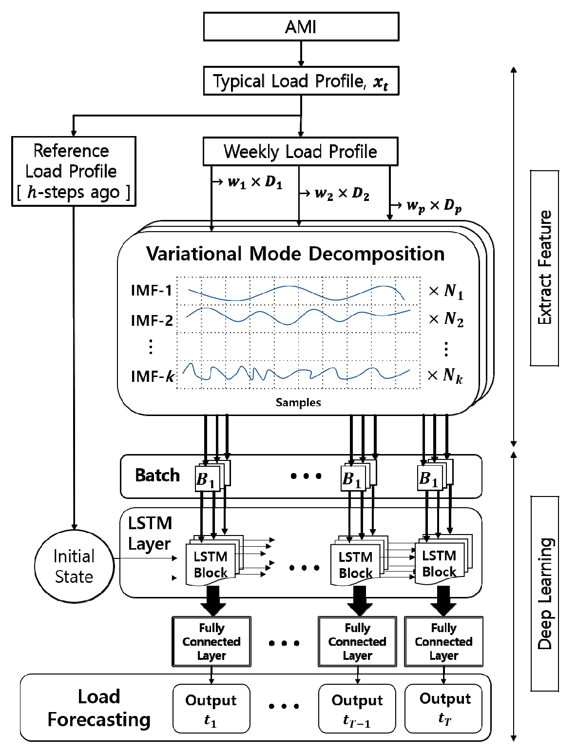
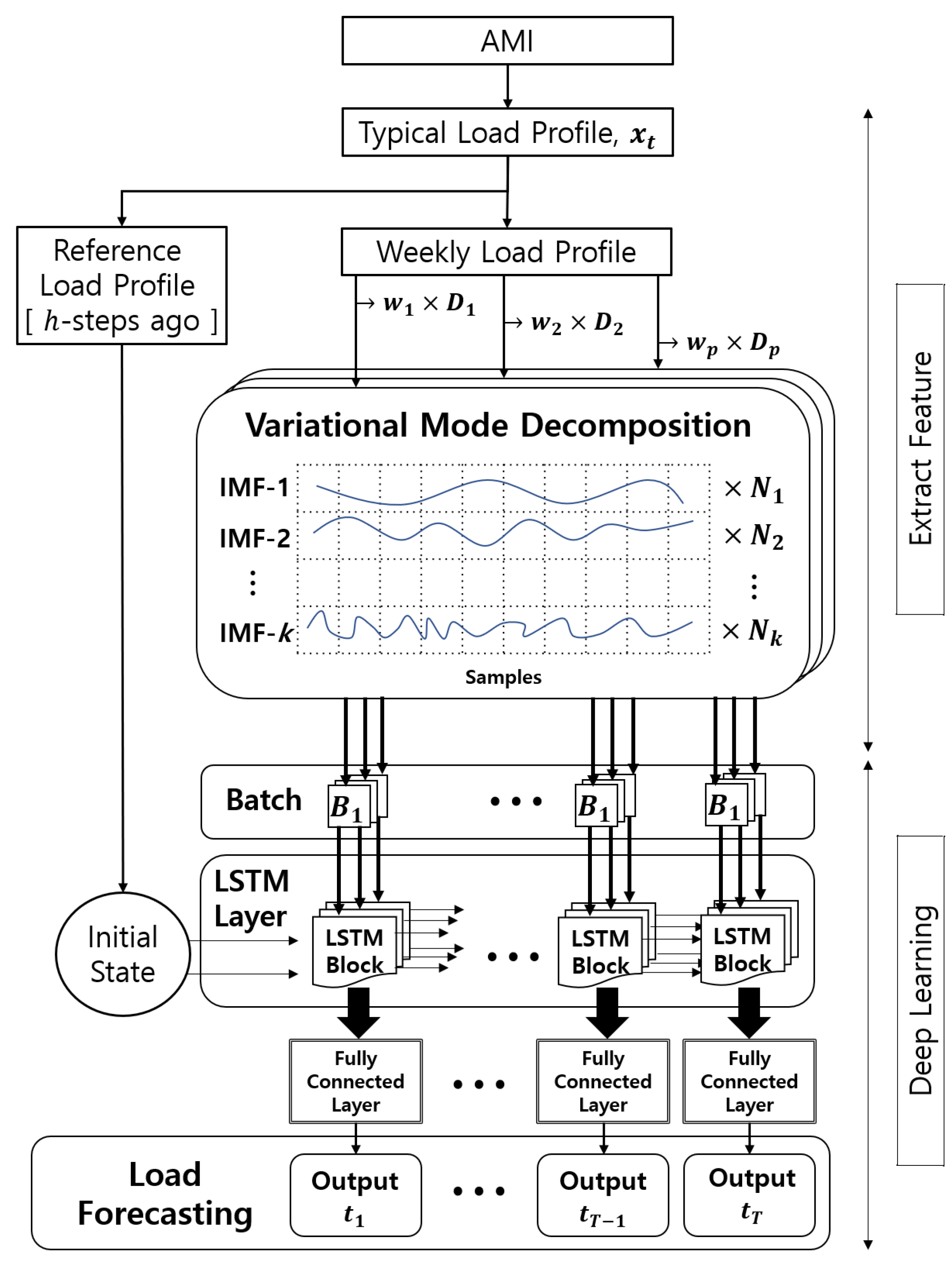
Figure 1 shows the proposed load profile decomposition method. The building load profile has similar weekday patterns, and the load is measured at 5-min intervals by AMI. To classify seasonal patterns, the typical load profile () of the building is decomposed on a weekly basis for weekly seasonality features (). The typical load profile is decomposed into two dimensions. The load variations can be extracted if they are periodic because the VMD decomposes the load profile in terms of the frequency (). Thus, all the IMFs exhibit periodic characteristics. As each IMF has a specific frequency, the VMD identifies periods that cannot be identified in the typical load profile and the weekly load profile. As a result, the typical load profile is decomposed into three-dimensional data according to time, weekly seasonality, and IMF-level. The feature decomposition process of the load profile contributes to the load characteristics without external data, such as the calendar information about holidays, temperature, and humidity.
2.5. Three-Step Regularization Process
The sampling of AMI used in this study is three-times larger than that of conventional AMI, which collects data at 15-min intervals. In addition, as the load profile is decomposed into sub-profiles, the sub-profiles that have detailed frequency characteristics can be learned as the input variables, but the number of input variables increases. As the number of input variables increases, the curse of dimensionality degrades the learning ability because the number of hidden nodes increases. As a result, the number of hidden layers is increased to solve the curse of dimensionality, but this causes the vanishing gradient problem. Moreover, without feature selection, overfitting occurs. The learned hypothesis may fit the training set very well, but it cannot be extended to new samples. In addition, without the normalization process, the covariate shift problem degrades performance. The covariate shift, which refers to the change in the distribution of the input variables present in the training and test data, should be prevented. Therefore, the proposed method includes a three-step regularization to solve each of the above-mentioned problems. First, the delay factor of weekly data is estimated. Although a large amount of data can be beneficial for deep learning, the distant past data can result in overfitting problems and increase the computation time. A similar problem was addressed in [36] to solve the dependence on distant historical data. In [36], a decay factor was used to solve the long-term dependency problem of NARX-RNN.
In this paper, the weekly decay’s exponent by a factor is proposed as Equation (3):
where p is the number of weeks, which gives high weights to nearby weekly data in time and lower weights to distant weekly past data.
Secondly, the separated IMF signals () are normalized against the original signal size (). This is because these signals correspond to residual noise such as frequencies that are too high or too low to be identified in a certain pattern. The IMF normalization process is performed to identify features that degrade learning. The IMF normalization factor given by Equation (4) and is the number of samples of the weekly data.
Finally, as the number of hidden layers increases, the internal covariance can be shifted. The internal covariate shift causes the distribution of the training set and test set to differ, which can lead to local points. Batch normalization (BN) is used to address internal covariate shift. BN normalizes the output of a previous activation layer by subtracting the batch mean and dividing by the batch standard deviation. The advantages of BN are (1) fast learning, (2) less careful initialization, and (3) a regularization effect. BN is one of the regularization techniques used in the deep learning field [41,42]. The regularization process contributes to the accuracy of the load forecasting and the optimization of the model by applying a high weight to the input data having the most definite period, reducing dependency on the past distant data and avoiding the covariate shift of the data group. The three-step regularization process increases the accuracy of the load forecasting by minimizing problems that can occur when several inputs are learned.
3. Deep Learning
Deep learning is one of the machine learning techniques that proposes to model high-level abstractions in data by using ANN architectures composed of multiple non-linear transformations. Deep learning refers to stacking multiple layers of neural networks and relying on stochastic optimization to perform efficient machine learning tasks. To take advantage of deep learning, three technical constraints must be solved. The three technical constraints are (1) the lack of sufficient data, (2) the lack of computing resources for a large network size, and (3) the lack of an efficient training algorithm. Recently, these constraints were solved by the development of big data applications, the Internet-of-Things, and high performance smart computing [37,38,39]. One of the most efficient deep learning processes is RNN.
RNNs are fundamentally different from traditional feed-forward neural networks; RNNs have a tendency to retain information acquired through subsequent time-stamps. This characteristic of RNNs is useful for load forecasting. Even though RNNs have good approximation capabilities, they are not fit to handle long-term dependencies of data. Learning long-range dependencies with RNNs is challenging because of the vanishing gradient problem. The increase in the number of layers and the longer paths to the past cause the vanishing gradient problem because of the back-propagation algorithm, which has the very desirable characteristic of being very flexible, although causes the vanishing gradient problem [30,32,33,34].
3.1. Long Short-Term Memory Neural Networks
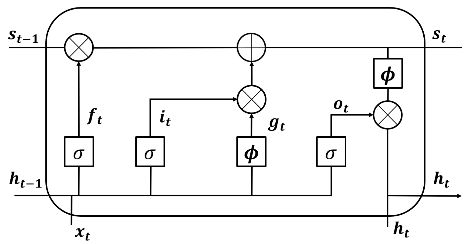
The long-short term memory network has been employed to approach the best performance of state-of-the-art RNNs. The problem of the vanishing gradient is solved by replacing nodes in the RNN with memory cells and a gating mechanism. Figure 2 shows the LSTM block structure. The overall support in a cell is provided by three gates. The memory cell state interacts with the intermediate output . The sub-sequent input determines whether to remember or forget the cell state. The forget gate determines the input for the cell state using the sigmoid function. The input gate , input node , and output node determine the values to be updated by each weight matrix, where represents the sigmoid activation function, while represents the tanh function. The weight matrices in the LSTM network model are determined by the back-propagation algorithm [37,38,39,40,41,42].
The LSTM has become the state-of-the-art RNN model for a variety of deep learning techniques. Several variants of the LSTM model for recurrent neural networks have been proposed. Variant LSTM models have been proposed to improve performance by solving issues such as computation time and the model complexity of the standard LSTM structure. Among the variants, the GRU maintains performance by simplifying the structure with an update gate that is coupled with an input gate and forget gate. The structure of the GRU is advantageous for forecasting in a large-scale grid to reduce calculation time [42]. In [45], variants of the LSTM architecture were designed and their performances were compared through implementation. The results revealed that none of the variants of LSTM could improve upon the standard LSTM. In other words, a clear winner could not be declared. Therefore, the popular LSTM networks are used in this study [45,46].
3.2. Nonlinear Autoregressive Network with Exogenous Inputs
NARX RNNs and LSTM solve the vanishing gradient problem with different mechanisms. NARX RNNs allow delays from the distant past layer, but this structure increases computation time and has a small effect on long-term dependencies. The LSTM solves the vanishing gradient problem by replacing nodes in the RNN with memory cells and a gating mechanism [36].
4. Experiments
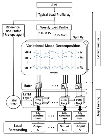
This section describes the process used to obtain time series models for load forecasting. Figure 3 shows the proposed load forecasting model using LSTM with multi-decomposition for feature extraction. We will discuss each step in detail.
4.1. Prediction of the Time Scale
Reference load profiles reflect the load profiles that are close to real-time load profiles before h steps ago, where h determines the prediction time scales, which depend on the purpose of the load forecasting. STLF techniques can be used for a variety of purposes by enabling smaller scales and faster prediction. USTLF, which predicts the load within a few minutes to one hour, can be used for electricity theft detection or can provide information for emergency power supply [47]. STLF, which predicts the load from one hour to a day, can be used for electricity transactions or economic dispatch of renewable energy resources [2].
4.2. Extract Feature Layer
Through the multi-decomposition method, the features of time-series data are extracted. The number of decomposition levels (K) is 10, which is the value obtained when the decomposition loss rate is 0.1% or less. The weight of the weekly load profile () considers the trend of load patterns according to seasonal changes. Each IMF decomposed through the VMD has a frequency characteristic and is normalized to make the feature stand out ().
4.3. Long Short-Term Memory Layer
The LSTM can capture long-term dependencies in time-stamps; therefore, it can address the vanishing gradient problems. In the proposed method, the number of hidden layers increases due to the decomposition of input data, but the vanishing gradient problem is solved through the memory cell structure with three-step regularization. In addition, to minimize the covariate shift problem, batch normalization is performed prior to the activation phase of the input. IMFs and reference load profiles are trained at each LSTM layer and have predictive values, all of which are summed to predict the load profile.
4.4. Model Construction
4.4.1. Hyperparameter Tuning and Training Options
The LSTM model has several hyperparameters such as the number of input neurons, hidden layers, input window size, number of epochs, regularization weight, batch size, and learning rate. The window size of input and output parameters depends on the time scale of load forecasting. The input neuron parameter is determined by the dimensions of the input data. The input dimension of the proposed method is 11, which is the sum of the reference profile and 10 IMF signals. We selected the hyperparameters and used ADAM optimization, one of the optimization techniques used in deep learning [30,31,32,33,34,35,36,37,38,39,40].
4.4.2. Training and Testing
The overall AMI dataset of each day is divided into a ratio of 70:15:15 for the purposes of model training, validation, and testing, respectively.
4.4.3. Performance Measures
The root mean squared error (RMSE) is used to compare differences between the predicted value and measured value and is computed for T (which is the number of samples of the weekly load profile) different predictions as the square root of the mean of the squares of the deviations:
The mean absolute error (MAE) is one of a number of ways of comparing forecasts with their eventual outcomes.
The mean absolute percent error (MAPE) is also widely used to evaluate accuracy. Accuracy can be compared via MAPE using percentages when the scale of the loads is different [37,38,39,40].
5. Load Profile Analysis by Multi-Decomposition Methods
5.1. Weekly Seasonality
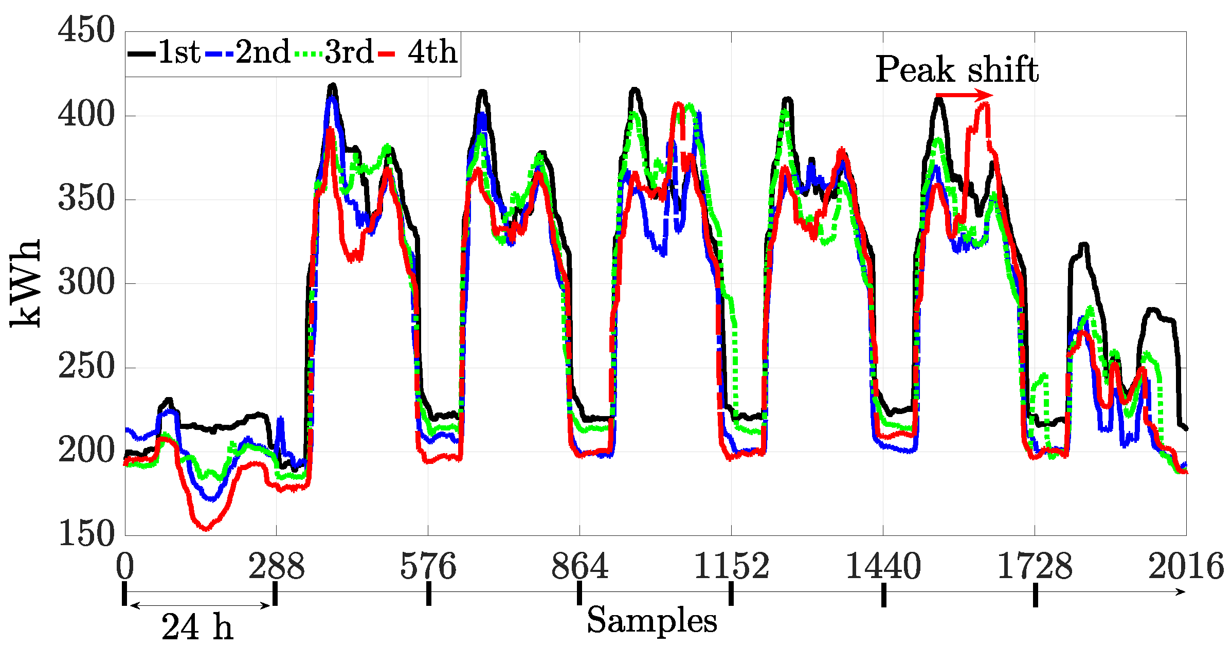
This study used real-world load profile data from the R&D business building that utilized enhanced AMI for demand side management. Figure 4 shows the real-world load profile of the business building. The building generates 288 samples per day, 2016 samples per week, and 8640 samples per month. The load profile is measured and stored in data storage.
The electrical load profile of the office building is usually light on weekends compared to weekdays because energy is consumed according to the business schedule. In contrast to those of residential load profile patterns, energy the increase and decrease times of office building load profiles are related to commute time and have similar daily characteristics. Figure 4 shows a typical profile for building electricity load over one week, from which a clear weekly seasonality pattern can be observed. The weekly load pattern is quite similar over four weeks, with a weekly average correlation of 0.93. Therefore, many studies have proposed load forecasting methods using weekly statistical methods or dividing the time series data into holidays, weekends, and weekdays [4,5].
However, the process of dividing the time series data in a database into weekdays, weekends, and holidays is inefficient because the calendar information may not be provided in advance, and each consumer group may have different days off. Moreover, the simple method of dividing the data into weekdays and holidays cannot capture the periodicity of the load profile such as the commute time and periodic power system on/off states. In Figure 4, the fourth week load pattern deviates somewhat from the previous pattern, with significant peak load shift in the afternoon, particularly on Wednesday and Friday (average correlations for Wednesday and Friday are 0.82 & 0.84, respectively). As the patterns deviated greatly on weekends (the weekend average correlation is 0.71), it is difficult to predict accurately energy consumption using daily statistical data alone. Therefore, feature extraction from the load profile is required to capture periodic components caused by commuting time, meal times, thermal control change, elevator system operation, etc.
5.2. Comparison of Decomposition Performance
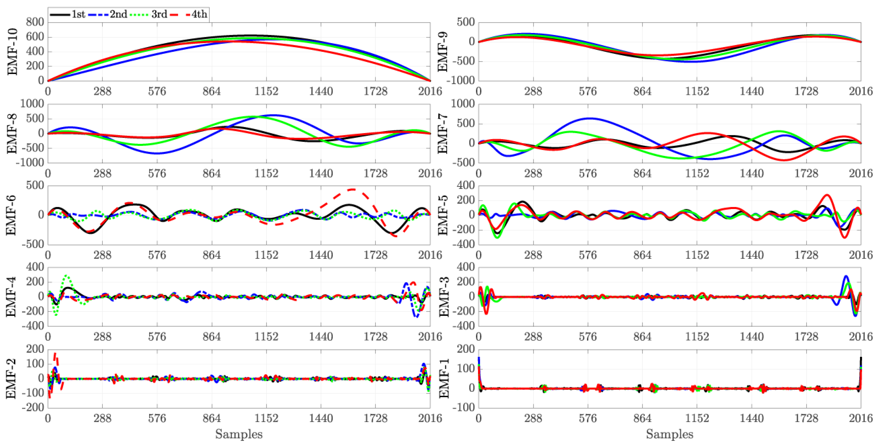
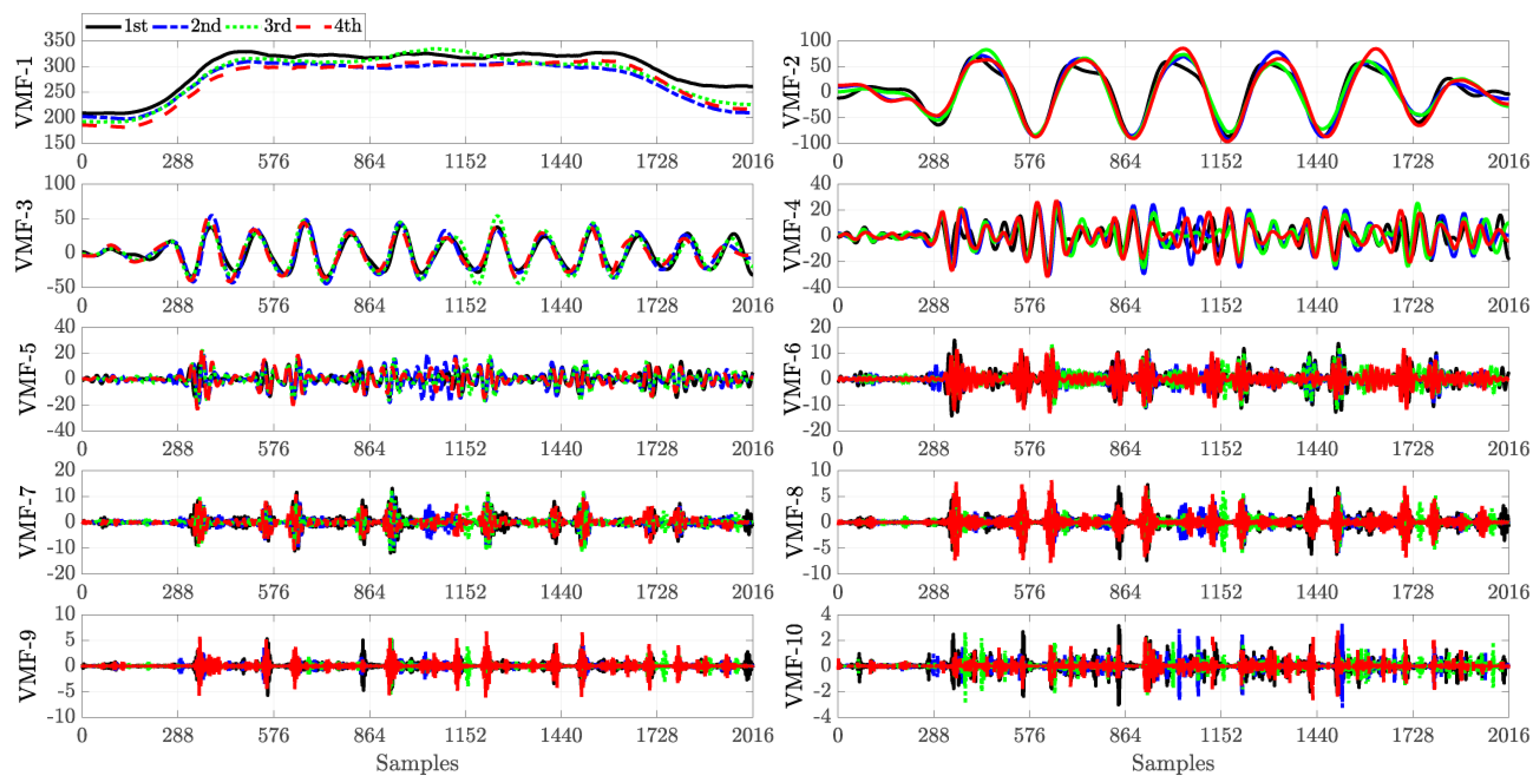
Figure 5 and Figure 6 show the load profiles of Figure 4 decomposed by EMD and VMD, respectively, where each IMF of each load profile covers four weeks. To analyze various frequency components and preserve the signal energy, in EMD, the standard deviation as the stop criterion is determined as 0.1%; hence, the weekly load profiles are decomposed into 10 IMFs.
As EMD decomposes the signal using extrema envelopes (Figure 5), the results are similar to those obtained with a low pass filter. However, VMD is similar to a high pass filter, as it decomposes the load profile from low frequency components. VMD IMFs (VMFs) are band limited; hence, they are similar to harmonic components. Therefore, VMD efficiently identifies periodic characteristics in non-linear and non-stationary signals compared to EMD IMFs (EMFs).
The first VMF (VMF-1) is effectively the DC bias (Figure 6), i.e., the average daily load consumption. VMF-2 and VMF-3 show high correlation signal periodicities. Office buildings typically exhibit a commute period, and this appears in VMF-2. This R&D building has two peaks around the commute time, and this pattern appears in VMF-3. On the other hand, EMF-10 and EMF-9 show high correlation trends, whereas the other EMFs show low correlations. High frequency EMFs (EMF-5–EMF-10) also include end-point problems, whereas VMD decomposes the signal into band-limited signals; hence, VMFs have no end-point issues.
Table 1 shows the correlations for each IMF. The VMFs capture similar frequency signals better than the EMFs and decompose high frequency signals well. As VMD is done mathematically, the correlation between VMFs is gradually reduced, whereas EMD IMFs are irregular. Therefore, in the case of high sampling or short prediction time scales, VMD shows better performance than EMD because VMD can reflect the high frequency characteristics of the dataset.
In addition, VMD can remove the inherent noise. Actual AMI data have noise owing to the interference due to peripheral electronic devices. VMD can improve the accuracy of the load forecasting through the deep learning training and regularization process by reducing the weight of high frequencies that are susceptible to noise, such as VMF-8, VMF-9, and VMF-10, which have low correlation indices of less than 1%. The AMI used in this study has a three-times higher sampling than conventional AMI and can reduce the model uncertainty as more samples are measured. The proposed method reduces the prediction uncertainty by training the decomposed signal with the high sampling AMI.
6. Case Studies
The time series forecasting models were simulated on real-world datasets of business buildings. We conducted the case studies with different prediction models and prediction time scales. The weekly prediction results for one hour ahead load forecasting are shown in Figure 7.
6.1. Comparative Conventional Load Forecasting Models
To validate the efficacy of the proposed VMD-LSTM RNN, eight load forecasting models, including ARIMA, SVR, GPR, NARX, NARX with EMD, NARX with VMD, LSTM, LSTM with EMD, and LSTM with VMD, were compared under the same benchmarks (RMSE, MAE, and MAPE).
The ARIMA model has been used for time-series prediction. However, with the rise of machine learning, the GPR and SVR models are being utilized. To account for seasonality in an ARIMA model, three hyperparameters were used: autoregression, stationarity, and moving average. The GPR model uses statistical hyperparameters, including variance and length, whereas the SVR model depends on kernel parameters, a penalty factor, and insensitive zone thickness. The ARIMA, GPR, and SVR models are trained through cross-validation and ADAM optimization or particle swarm optimization [2,26,27,28,29]. To compare the performance of the RNNs, we compared the results of applying two decomposition methods to the NARX and LSTM models The prediction results of all models are shown in Figure 7, and the prediction accuracy by day of the week is shown in Figure 8. Table 2 also summarizes the performance at different time scales.
6.2. Weekly Load Forecasting
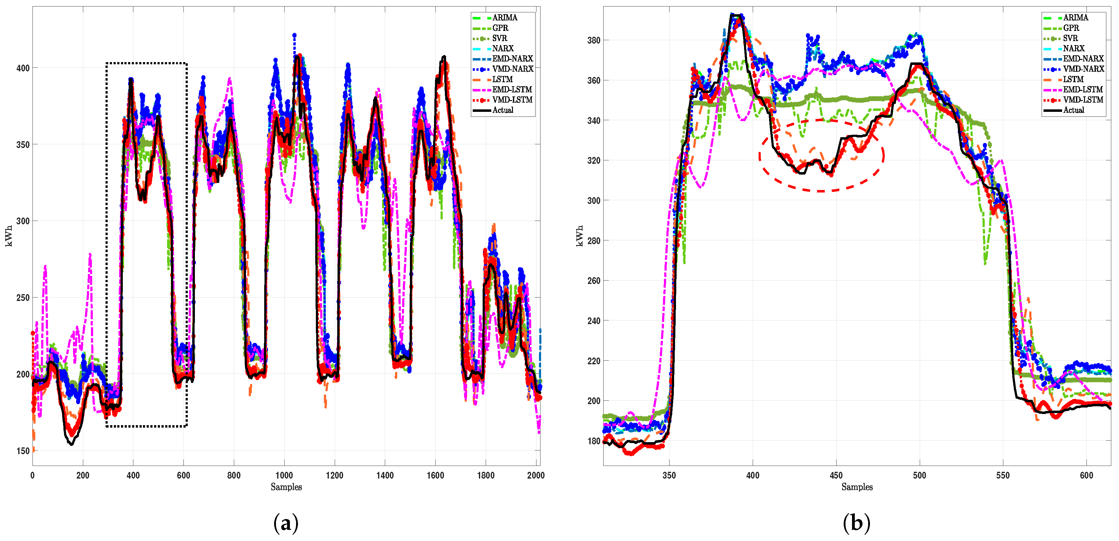
Figure 7 illustrates the STLF for building load with one hour ago (12 steps ahead). To check the performance of the proposed method based on VMD and LSTM, the prediction results of different methods were compared. A closer look at the prediction results reveals the Monday load forecasting in Figure 7b. The proposed model showed robust performance under abrupt load increases and decreases in 400 samples and 500 samples, respectively. Conventional models exhibited conservative changes to sudden load changes, and EMD-LSTM exhibited excessive weight changes.
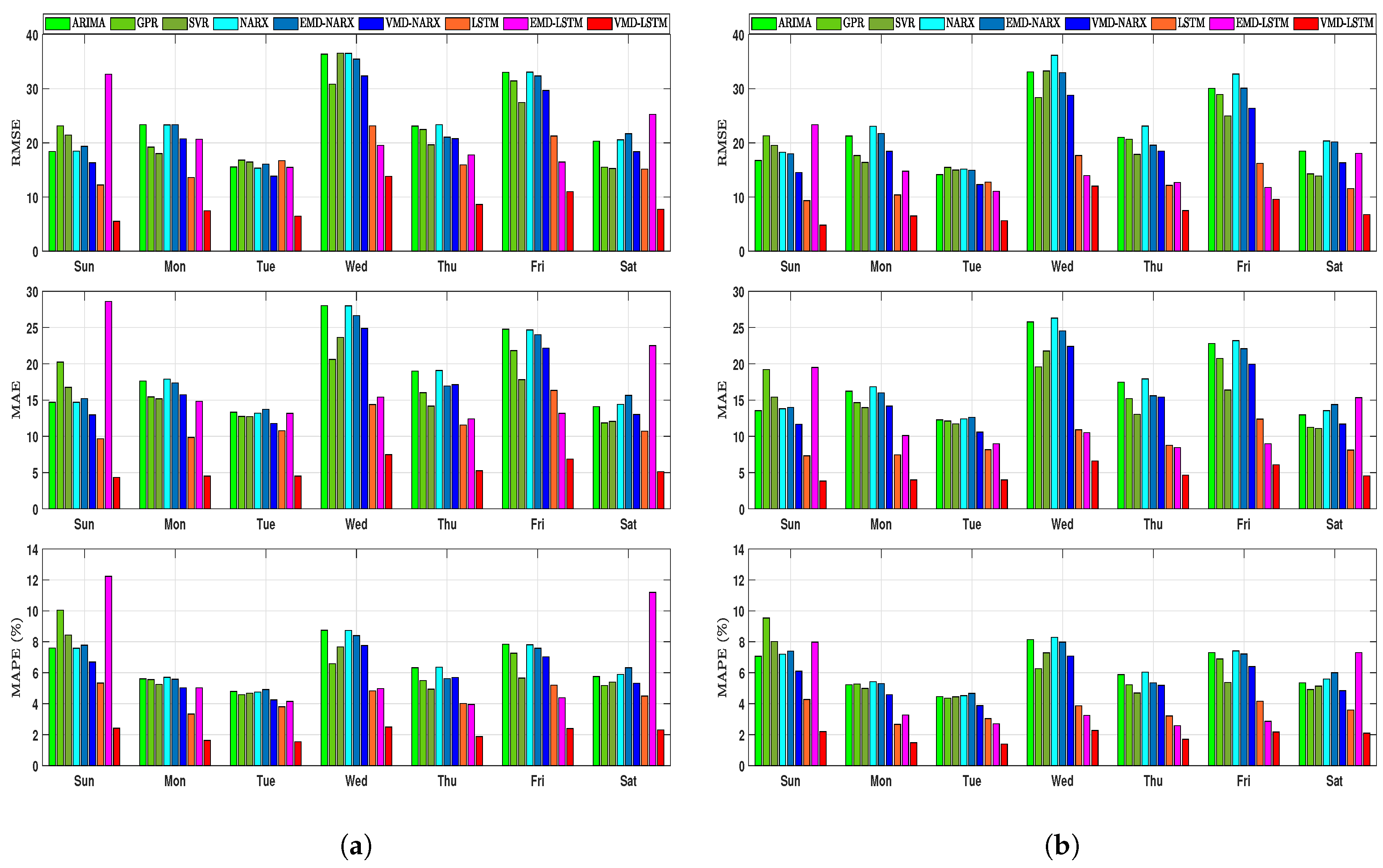
Figure 8 shows the average predictive error of the different methods. The result of load forecasting with one-month AMI data is shown in Figure 8a, and Figure 8b is the prediction result with three months of AMI data. There are distinct load characteristics for each day of the week. EMD-LSTM had large errors with an RMSE of 32.68 kWh, MAE of 28.61 kWh, and MAPE of 12.24% on Sunday in Figure 8a. However, if the size of the dataset is sufficiently large or the prediction time scale is long enough, the initial error can be corrected. When the data are insufficient with a short time scale, the input of the reference load profile (which is measurement data at the maximum observable time before load forecasting) can be a dominant feature of machine learning, which causes a large error. Figure 8 shows that, if the LSTM correctly decomposed periodic features, it had high accuracy even with small amounts of data, but if there was an error in the feature, the prediction error also increased because of the memory cell structure of LSTM.
VMD can reflect more dominant patterns than EMD with distinct periodicity. The performance difference of decomposition between EMD and VMD is shown in Figure 4 and Figure 5. The RNNs using VMD showed performance improvements. However, there was a difference in performance improvement between NARX and LSTM because the vanishing gradient problem was solved differently, where NARX used the delay factor and LSTM had the memory cell structure. As LSTM preserved characteristics of dominant features through the memory cell, LSTM showed higher accuracy than NARX in STLF.
The MAPE of VMD-LSTM was around 2%. In the weekly comparison, the least error occurred on Tuesday: RMSE of 6.49 kWh, MAE of 3.98 kWh, and MAPE of 1.48%. This was because the correlation between days of the week was the highest on Tuesday. On the other hand, there was a large error on Wednesday and Friday because the correlation was relatively lower than on other days of the week.
The proposed VMD-LSTM reflecting the mixed periodic pattern of the load profile based on multi-decomposition with deep learning had the lowest error.
6.3. Benchmark for Different Prediction Time Scales
Finally, in this section, we analyze the accuracy of the load forecasting methods for the case study considering different prediction time scales (5 m, 1 h, 3 h, 24 h, 48 h, 72 h). The accuracy results are summarized in Table 2. The best accuracies were obtained for the shortest prediction time scale (5 m) for all models. The proposed model, VMD-LSTM, showed the best accuracy with an MAE of 1.95 kWh, RMSE of 4.28 kWh, and MAPE of 0.71%.
In addition, EMD-LSTM and VMD-LSTM showed better accuracy on the previous day when compared to the 36 steps ahead (3 h) and one day to three days ahead (24 h, 48 h, 72 h) time scales. The 24 h, 48 h, and 72 h cases show that RNN-based models had higher accuracies than ARIMA or GPR, but eventually showed similar errors, and their performances were saturated. This result was obtained because the reference load profile was learned as a dominant input according to the prediction time scale to reflect the power consumption trend, so the 288 steps ahead case and 576 steps ahead case, which had similar patterns, were slightly more accurate than the 36 steps ahead case (3 h).
7. Conclusions
This paper proposes short-term load forecasting using deep learning based on multi-decomposition. The results of the proposed approach were validated by applications to real-world data from a business building, and the performance of the proposed approach was assessed by comparing the predicted results with those of other models.
To monitor small-scale load and demand side management, an enhanced AMI that provides three-times more sample data points per hour than conventional AMI was used, increasing the accuracy of the load forecasting using deep learning. In this study, to detect the features of the load profile, the load profile was decomposed by a weekly seasonality and variational mode decomposition. Two decomposition methods can identify features such as seasonality, load increase/decrease pattern, and periodicity without any external data, such as temperature.
The three-step regularization process reduced the long-term dependency, overfitting, and covariate shift problem caused by feature decomposition, which increases the data samples and dimensions. The results also reveal the effectiveness of the long short-term memory neural networks based on variational mode decomposition with different prediction time scales. We expect the proposed method to be a key technique for demand side management, electrical power theft detection, energy storage system scheduling, and energy trading platforms in future smart grids.
Author Contributions
S.H.K. developed the main idea and designed the proposed model; he conducted the simulation studies and wrote the paper with the support of G.L. and G.-Y.K. under the supervision of the corresponding author, Y.-J.S. D.-I.K. contributed to the editing of the paper. All authors have read and approved the final manuscript.
Acknowledgments
This work was supported by a National Research Foundation of Korea (NRF) grant funded by the Ministry of Science, ICT & Future Planning (No. NRF-2017R1A2A1A05001022) and the framework of the international cooperation program managed by the NRF of Korea (No. NRF-2017K1A4A3013579). This research was also supported by the Korea Electric Power Corporation (KEPCO) (No. R18XA05).
Conflicts of Interest
The authors declare no conflicts of interest.
Nomenclature
| AMI | advanced measuring infrastructure |
| ANN | artificial neural network |
| LSTM | long short-term memory |
| EMD | empirical mode decomposition |
| VMD | variational mode decomposition |
| LTLF | long-term load forecasting |
| MTLF | medium-term load forecasting |
| STLF | short-term load forecasting |
| USTLF | ultra-short-term load forecasting |
| DSM | demand side management |
| ARIMA | auto-regressive integrated moving average |
| GPR | Gaussian processing regression |
| GRU | gated recurrent unit |
| SVR | support vector regression |
| RNN | recurrent neural network |
| NARX | nonlinear autoregressive exogenous |
| CNN | convolutional neural network |
| IMFs | intrinsic mode functions |
| k | the mode index |
| intrinsic mode | |
| weekly load profile | |
| w | frequency of mode |
| K | the total number of modes |
| the typical load profile | |
| the load weekly seasonality feature | |
| IMF of the load weekly seasonality feature | |
| the Dirac distribution | |
| the weekly decay’s exponent factor | |
| the IMF normalization factor | |
| BN | batch normalization |
| the memory cell state of LSTM | |
| the forget gate of LSTM | |
| the input gate of LSTM | |
| the input node of LSTM | |
| the output gate of LSTM | |
| the output value of LSTM | |
| RMSE | root mean squared error |
| MAE | mean absolute error |
| MAPE | mean absolute percent error |
| VMF | variational mode function |
| EMF | empirical mode function |
References
- Ekonomou, L.; Christodoulou, C.A.; Mladenov, V. A short-term load forecasting method using artificial neural networks and wavelet analysis. Int. J. Power Syst. 2016, 1, 64–68. [Google Scholar]
- Mirowski, P.; Chen, S.; Ho, T.K.; Yu, C.-N. Demand forecasting in smart grids. Bell Syst. Tech. J. 2014, 18, 135–158. [Google Scholar] [CrossRef]
- Zhang, X. Short-term load forecasting for electric bus charging stations based on fuzzy clustering and least squares support vector machine optimized by wolf pack algorithm. Energies 2018, 11, 1449. [Google Scholar] [CrossRef]
- Fiot, J.-B.; Dinuzzo, F. Electricity demand forecasting by multi-task learning. IEEE Trans. Smart Grid 2018, 9, 544–551. [Google Scholar] [CrossRef]
- Dahl, M.; Brun, A.; Kirsebom, O.; Andresen, G. Improving short-term heat load forecasts with calendar and holiday data. Energies 2018, 11, 1678. [Google Scholar] [CrossRef]
- Teeraratkul, T.; O’Neill, D.; Lall, S. Shape-based approach to household electric load curve clustering and prediction. IEEE Trans. Smart Grid 2018, 9, 5196–5206. [Google Scholar] [CrossRef]
- Wang, Y.; Zhang, N.; Chen, Q.; Kirschen, D.S.; Li, P.; Xia, Q. Data-driven probabilistic net load forecasting with high penetration of behind-the-meter pv. IEEE Trans. Power Syst. 2018, 33, 3255–3264. [Google Scholar] [CrossRef]
- Haben, S.; Singleton, C.; Grindrod, P. Analysis and clustering of residential customers energy behavioral demand using smart meter data. IEEE Trans. Smart Grid 2016, 7, 136–144. [Google Scholar] [CrossRef]
- Stephen, B.; Tang, X.; Harvey, P.R.; Galloway, S.; Jennett, K.I. Incorporating practice theory in sub-profile models for short term aggregated residential load forecasting. IEEE Trans. Smart Grid 2017, 8, 1591–1598. [Google Scholar] [CrossRef]
- Hayes, B.P.; Gruber, J.K.; Prodanovic, M. Multi-nodal short-term energy forecasting using smart meter data. IET Gener. Transm. Dis. 2018, 12, 2988–2994. [Google Scholar] [CrossRef]
- Xie, J.; Chen, Y.; Hong, T.; Laing, T.D. Relative humidity for load forecasting models. IEEE Trans. Smart Grid 2018, 9, 191–198. [Google Scholar] [CrossRef]
- Xie, J.; Hong, T. Temperature scenario generation for probabilistic load forecasting. IEEE Trans. Smart Grid 2018, 9, 1680–1687. [Google Scholar] [CrossRef]
- Li, P.; Zhang, J.; Li, C.; Zhou, B.; Zhang, Y.; Zhu, M.; Li, N. Dynamic similar sub-series selection method for time series forecasting. IEEE Access 2018, 6, 32532–32542. [Google Scholar] [CrossRef]
- Lin, L.; Xue, L.; Hu, Z.; Huang, N. Modular predictor for day-ahead load forecasting and feature selection for different hours. Energies 2018, 11, 1899. [Google Scholar] [CrossRef]
- Xie, J.; Hong, T. Variable selection methods for probabilistic load forecasting: Empirical evidence from seven states of the united states. IEEE Trans. Smart Grid 2018, 9, 6039–6046. [Google Scholar] [CrossRef]
- Li, B.; Zhang, J.; He, Y.; Wang, Y. Short-term load-forecasting method based on wavelet decomposition with second-order gray neural network model combined with adf test. IEEE Access 2017, 5, 16324–16331. [Google Scholar] [CrossRef]
- Rafiei, M.; Niknam, T.; Aghaei, J.; Shafie-khah, M.; Catalão, J.P.S. Probabilistic load forecasting using an improved wavelet neural network trained by generalized extreme learning machine. IEEE Trans. Smart Grid 2018, 9, 6961–6971. [Google Scholar] [CrossRef]
- Auder, B.; Cugliari, J.; Goude, Y.; Poggi, J.-M. Scalable clustering of individual electrical curves for profiling and bottom-up forecasting. Energies 2018, 11, 1893. [Google Scholar] [CrossRef]
- Qiu, X.; Ren, Y.; Suganthan, P.N.; Amaratunga, G.A.J. Empirical mode decomposition based ensemble deep learning for load demand time series forecasting. Appl. Soft Comput. 2017, 54, 246–255. [Google Scholar] [CrossRef]
- Bedi, J.; Toshniwal, D. Empirical mode decomposition based deep learning for electricity demand forecasting. IEEE Access 2018, 6, 49144–49156. [Google Scholar] [CrossRef]
- Liu, H.; Mi, X.; Li, Y. An experimental investigation of three new hybrid wind speed forecasting models using multi-decomposing strategy and elm algorithm. Renew. Energy 2018, 123, 694–705. [Google Scholar] [CrossRef]
- Lahmiri, S. Comparing variational and empirical mode decomposition in forecasting day-ahead energy prices. IEEE Syst. J. 2017, 11, 1907–1910. [Google Scholar] [CrossRef]
- Dragomiretskiy, K.; Zosso, D. Variational mode decomposition. IEEE Trans. Signal Process. 2014, 62, 531–544. [Google Scholar] [CrossRef]
- Huang, N.; Yuan, C.; Cai, G.; Xing, E. Hybrid short term wind speed forecasting using variational mode decomposition and a weighted regularized extreme learning machine. Energies 2016, 9, 989. [Google Scholar] [CrossRef]
- Lin, Y.; Luo, H.; Wang, D.; Guo, H.; Zhu, K. An ensemble model based on machine learning methods and data preprocessing for short-term electric load forecasting. Energies 2017, 10, 1186. [Google Scholar] [CrossRef]
- Ruiz-Abellón, M.; Gabaldón, A.; Guillamón, A. Load forecasting for a campus university using ensemble methods based on regression trees. Energies 2018, 11, 2038. [Google Scholar] [CrossRef]
- Dong, Y.; Zhang, Z.; Hong, W.-C. A hybrid seasonal mechanism with a chaotic cuckoo search algorithm with a support vector regression model for electric load forecasting. Energies 2018, 11, 1009. [Google Scholar] [CrossRef]
- Li, M.-W.; Geng, J.; Hong, W.-C.; Zhang, Y. Hybridizing chaotic and quantum mechanisms and fruit fly optimization algorithm with least squares support vector regression model in electric load forecasting. Energies 2018, 11, 2226. [Google Scholar] [CrossRef]
- Sheng, H.; Xiao, J.; Cheng, Y.; Ni, Q.; Wang, S. Short-term solar power forecasting based on weighted gaussian process regression. IEEE Trans. Ind. Electron. 2018, 65, 300–308. [Google Scholar] [CrossRef]
- Manic, M.; Amarasinghe, K.; Rodriguez-Andina, J.J.; Rieger, C. Intelligent buildings of the future: Cyberaware, deep learning powered, and human interacting. IEEE Ind. Electron. Mag. 2016, 10, 32–49. [Google Scholar] [CrossRef]
- Li, C.; Ding, Z.; Yi, J.; Lv, Y.; Zhang, G. Deep belief network based hybrid model for building energy consumption prediction. Energies 2018, 11, 242. [Google Scholar] [CrossRef]
- Wang, Y.; Zhang, N.; Tan, Y.; Hong, T.; Kirschen, D.S.; Kang, C. Combining probabilistic load forecasts. IEEE Trans. Smart Grid 2018. Available online: https://arxiv.org/abs/1803.06730 (accessed on 5 November 2018). [CrossRef]
- Wang, J.; Gao, Y.; Chen, X. A novel hybrid interval prediction approach based on modified lower upper bound estimation in combination with multi-objective salp swarm algorithm for short-term load forecasting. Energies 2018, 11, 1561. [Google Scholar] [CrossRef]
- Sun, W.; Zhang, C. A hybrid ba-elm model based on factor analysis and similar-day approach for short-term load forecasting. Energies 2018, 11, 1282. [Google Scholar] [CrossRef]
- Ruiz, L.G.B.; Cuéllar, M.P.; Calvo-Flores, M.D.; Jiménez, M.D.C.P. An application of non-linear autoregressive neural networks to predict energy consumption in public buildings. Energies 2016, 9, 684. [Google Scholar] [CrossRef]
- DiPietro, R.; Rupprecht, C.; Navab, N.; Hager, G.D. Analyzing and exploiting narx recurrent neural networks for long-term dependencies. arXiv, 2017; arXiv:1702.07805. [Google Scholar]
- Bouktif, S.; Fiaz, A.; Ouni, A.; Serhani, M. Optimal deep learning lstm model for electric load forecasting using feature selection and genetic algorithm: Comparison with machine learning approaches. Energies 2018, 11, 1636. [Google Scholar] [CrossRef]
- Kong, W.; Dong, Z.Y.; Jia, Y.; Hill, D.J.; Xu, Y.; Zhang, Y. Short-term residential load forecasting based on lstm recurrent neural network. IEEE Trans. Smart Grid 2018. [Google Scholar] [CrossRef]
- Chen, K.; Chen, K.; Wang, Q.; He, Z.; Hu, J.; He, J. Short-term load forecasting with deep residual networks. IEEE Trans. Smart Grid 2018. Available online: https://arxiv.org/abs/1805.11956 (accessed on 5 November 2018). [CrossRef]
- Shi, H.; Xu, M.; Li, R. Deep learning for household load forecasting—A novel pooling deep rnn. IEEE Trans. Smart Grid 2018, 9, 5271–5280. [Google Scholar] [CrossRef]
- Kuo, P.-H.; Huang, C.-J. A high precision artificial neural networks model for short-term energy load forecasting. Energies 2018, 11, 213. [Google Scholar] [CrossRef]
- Wang, Y.; Liu, M.; Bao, Z.; Zhang, S. Short-term load forecasting with multi-source data using gated recurrent unit neural networks. Energies 2018, 11, 1138. [Google Scholar] [CrossRef]
- Merkel, G.; Povinelli, R.; Brown, R. Short-term load forecasting of natural gas with deep neural network regression. Energies 2018, 11, 2008. [Google Scholar] [CrossRef]
- Li, Y.; Huang, Y.; Zhang, M. Short-term load forecasting for electric vehicle charging station based on niche immunity lion algorithm and convolutional neural network. Energies 2018, 11, 1253. [Google Scholar] [CrossRef]
- Greff, K.; Srivastava, R.K.; Koutník, J.; Steunebrink, B.R.; Schmidhuber, J. LSTM: A search space odyssey. IEEE Trans. Neural Netw. Learn. Syst. 2017, 28, 2222–2232. [Google Scholar] [CrossRef] [PubMed]
- Chung, J.; Gulcehre, C.; Cho, K.; Bengio, Y. Empirical Evaluation of Gated Recurrent Neural Networks on Sequence Modeling. arXiv, 2014; arXiv:1412.3555. [Google Scholar]
- Zhan, T.-S.; Chen, S.-J.; Kao, C.-C.; Kuo, C.-L.; Chen, J.-L.; Lin, C.-H. Non-technical loss and power blackout detection under advanced metering infrastructure using a cooperative game based inference mechanism. IET Gener. Transm. Dis. 2016, 10, 873–882. [Google Scholar] [CrossRef]
Figure 1.
Load profile feature decomposition process.

Figure 2.
The structure of the LSTM.

Figure 3.
Deep-learning load forecasting based on the multi-decomposition method.

Figure 4.
The typical load profile of the business building.

Figure 5.
Weekly load profile decomposition using EMD (k = 10). EMF, EMD IMF.

Figure 6.
Weekly load profile decomposition using VMD (k = 10). VMF, VMD IMF.

Figure 7.
Actual and different load forecasting for a week. (a) Weekly load forecasting; (b) Monday load forecasting.
Figure 7.
Actual and different load forecasting for a week. (a) Weekly load forecasting; (b) Monday load forecasting.

Figure 8.
Benchmarks of different models. (a) One-month AMI data; (b) Three-month AMI data.


Table 1.
Correlation index comparison of EMD and VMD.
| Decomposition | IMF | |||||||||
|---|---|---|---|---|---|---|---|---|---|---|
| 1 | 2 | 3 | 4 | 5 | 6 | 7 | 8 | 9 | 10 | |
| EMD | 0.58 | 0.42 | 0.40 | 0.28 | 0.46 | 0.35 | 0.02 | 0.43 | 0.82 | 0.96 |
| VMD | 0.98 | 0.83 | 0.80 | 0.63 | 0.53 | 0.26 | 0.15 | 0.01 | −0.02 | −0.02 |
Table 2.
Load forecasting errors of different models.
| Prediction Horizon | Index | ARIMA | GPR | SVR | NARX | EMD NARX | VMD NARX | LSTM | EMD LSTM | VMD LSTM |
|---|---|---|---|---|---|---|---|---|---|---|
| 1 step ahead (5 min) | MAE | 7.45 | 6.03 | 3.43 | 7.52 | 7.33 | 3.25 | 2.92 | 5.53 | 1.95 |
| RMSE | 11.77 | 10.21 | 6.89 | 11.89 | 11.21 | 6.62 | 4.98 | 8.72 | 4.28 | |
| MAPE (%) | 3.46 | 2.67 | 1.96 | 3.61 | 3.39 | 1.84 | 1.12 | 2.21 | 0.71 | |
| 12 steps ahead (1 h) | MAE | 17.28 | 16.11 | 14.76 | 17.71 | 17.02 | 15.12 | 9.01 | 11.69 | 4.81 |
| RMSE | 22.12 | 20.94 | 20.12 | 24.12 | 22.49 | 19.31 | 12.87 | 15.08 | 7.53 | |
| MAPE (%) | 6.20 | 6.06 | 5.70 | 6.35 | 6.27 | 5.43 | 3.54 | 4.27 | 1.90 | |
| 36 steps ahead (3 h) | MAE | 57.14 | 53.96 | 48.72 | 58.85 | 56.54 | 50.69 | 30.25 | 38.52 | 16.27 |
| RMSE | 64.50 | 61.35 | 59.31 | 70.64 | 66.80 | 56.38 | 38.05 | 43.66 | 22.40 | |
| MAPE (%) | 20.62 | 19.91 | 18.17 | 21.79 | 20.97 | 20.03 | 11.63 | 14.26 | 6.01 | |
| 288 steps ahead (24 h) | MAE | 51.22 | 48.55 | 43.25 | 52.68 | 51.50 | 45.12 | 28.19 | 32.65 | 15.60 |
| RMSE | 59.38 | 58.81 | 56.88 | 58.12 | 57.24 | 56.85 | 35.98 | 37.38 | 21.80 | |
| MAPE (%) | 18.90 | 17.91 | 16.13 | 19.16 | 19.06 | 16.71 | 10.62 | 11.78 | 5.75 | |
| 576 steps ahead (48 h) | MAE | 57.24 | 52.87 | 46.57 | 57.48 | 55.65 | 48.23 | 28.60 | 32.48 | 15.85 |
| RMSE | 63.28 | 60.31 | 59.72 | 62.51 | 61.49 | 57.53 | 36.24 | 42.27 | 22.11 | |
| MAPE (%) | 22.08 | 19.72 | 17.76 | 21.49 | 20.99 | 17.18 | 10.92 | 12.18 | 5.89 | |
| 864 steps ahead (72 h) | MAE | 60.45 | 58.55 | 51.92 | 59.75 | 59.01 | 53.44 | 29.12 | 34.37 | 16.09 |
| RMSE | 68.24 | 62.42 | 58.35 | 67.38 | 66.26 | 58.72 | 36.85 | 43.52 | 22.18 | |
| MAPE (%) | 24.14 | 21.76 | 18.72 | 22.43 | 21.19 | 19.05 | 11.05 | 12.86 | 5.96 |
© 2018 by the authors. Licensee MDPI, Basel, Switzerland. This article is an open access article distributed under the terms and conditions of the Creative Commons Attribution (CC BY) license (http://creativecommons.org/licenses/by/4.0/).
Share and Cite
MDPI and ACS Style
Kim, S.H.; Lee, G.; Kwon, G.-Y.; Kim, D.-I.; Shin, Y.-J. Deep Learning Based on Multi-Decomposition for Short-Term Load Forecasting. Energies 2018, 11, 3433. https://doi.org/10.3390/en11123433
AMA Style
Kim SH, Lee G, Kwon G-Y, Kim D-I, Shin Y-J. Deep Learning Based on Multi-Decomposition for Short-Term Load Forecasting. Energies. 2018; 11(12):3433. https://doi.org/10.3390/en11123433
Chicago/Turabian StyleKim, Seon Hyeog, Gyul Lee, Gu-Young Kwon, Do-In Kim, and Yong-June Shin. 2018. "Deep Learning Based on Multi-Decomposition for Short-Term Load Forecasting" Energies 11, no. 12: 3433. https://doi.org/10.3390/en11123433
Note that from the first issue of 2016, this journal uses article numbers instead of page numbers. See further details here.