The Impact of Behavioral and Structural Remedies on Electricity Prices: The Case of the England and Wales Electricity Market


Department of Economics, Management and Humanities, Faculty of Electrical Engineering, Czech Technical University in Prague, Technická 2, 166 27 Prague 6, Czech Republic
Energies 2018, 11(12), 3420; https://doi.org/10.3390/en11123420
Submission received: 7 November 2018
/
Revised: 29 November 2018
/
Accepted: 4 December 2018
/
Published: 6 December 2018
(This article belongs to the Section C: Energy Economics and Policy)
Abstract
:During the liberalization process the UK regulatory authority introduced a behavioral remedy (through price-cap regulation) and structural remedy (through divestment series) in order to mitigate an exercise of market power and lower the influence of incumbent producers on wholesale electricity prices. We study the impact of these remedies on the dynamics of the wholesale electricity price during the peak-demand period over trading days. An extended autoregressive and autoregressive conditional heteroscedasticity (AR–ARCH) model with a novel skew generalized error distribution is used. This distribution allows one to capture the features of asymmetry, excess kurtosis, and heavy tails. The model is extended to include individual incumbent producers’ market shares and other explanatory variables reflecting seasonal patterns and regulatory regimes. We find that the structural remedy was more successful than the behavioral remedy because the effect of market share of the previously larger incumbent producer on the wholesale price is statistically insignificant. Moreover, after the second series of divestments, price volatility reduced.
1. Introduction
Great Britain was the first among the OECD countries to liberalize its electricity supply industry. The aim of liberalization was to introduce competition into electricity wholesale generation. Similarly, other electricity markets in Europe completed liberalization in 2007 [1]. The production level of the electricity supply industry in Great Britain consisted of several firms where National Power (NP) and PowerGen (PG) had dominant positions. During the liberalization process, the regulatory authority, Office of Electricity Regulation (later renamed the Office of Gas and Electricity Markets), introduced a behavioral remedy (through price-cap regulation) and a structural remedy (through divestment series) at different points of time, which were targeted at the NP and PG producers.
Price-cap regulation set an explicit ceiling on time-weighted and demand-weighted annual average prices charged for electricity production by the two incumbent electricity producers: NP (the larger producer) and PG (the smaller producer), which together sometimes produced more than 70% of electricity in the early 1990s. Later, divestment series were introduced in order to lower the influence of the incumbent producers on wholesale electricity prices. Following divestment series, the market shares of the incumbent electricity producers declined. Market share is an important factor affecting a firm’s behavior and eventually market prices. These are summarized in Figure 1.
Generally, there is no consensus regarding the optimal remedy choice (behavioral or structural) to address market failures. Behavioral remedies try to redress specific conduct in a context where incentives remain essentially unchanged. Structural remedies, on the other hand, are aimed at changing the incentives of the firm(s) in the market, which is achieved once the structural remedies are implemented [8].
European Union antitrust policy prioritizes the imposition of behavioral remedies above structural remedies because antitrust investigations typically concern infringements which are behavioral in nature. In the United States, on the other hand, there is a preference for structural remedies because they are simple and relatively easy to administer [9].
However, in 2008, following the investigation of E.ON (the world’s largest utility company, Essen, Germany) on the German wholesale electricity market, for the first time the European Commission decided to apply a structural remedy. Specifically, it was agreed that E.ON would divest 5000 MW of generation capacity representing about 20% of the company’s German generation portfolio [10].
As discussed in [11], the advantage of a structural remedy is that it allows for the reduction of a firm’s market share and the prevention of the emergence or strengthening of a dominant position. Moreover, there will be no need for subsequent monitoring and enforcement. According to [12], structural remedies should only be imposed either where there is no equally effective behavioral remedy or where any equally effective behavioral remedy would be more burdensome for the firm concerned than the structural remedy.
The wholesale electricity market in England and Wales presents an interesting case study where the regulatory authority introduced behavioral and structural remedies at different points of time. This enables us to compare the impact of each of the remedy on wholesale electricity prices.
Most of the research on this market focuses, however, on the analysis of market power exercised by the dominant producers. Little research has been done on the effect of reforms on wholesale electricity prices. The authors in [6] analyze nonparametrically the volatility of weekly average wholesale electricity prices. The authors in [13] study the effect of institutional changes and reforms on the dynamics of daily average wholesale electricity prices using the generalized error distribution, which allows one to capture the features of heavy tails and excess kurtosis (that is, kurtosis above 3). For the prices in other electricity markets, a Student’s t distribution and a skew Student’s t distribution have been used (see, for example, [14,15], respectively), which are valid to use when kurtosis is below 3. Indeed, as described in Figure 2b, a (skew) Student’s t distribution has a peak lower than in a normal distribution for which kurtosis is 3.
In this paper, we use an extended autoregressive and autoregressive conditional heteroscedasticity (AR–ARCH) model with a novel skew generalized error distribution (SGED) in order to study the dynamics of the wholesale electricity price during the peak-demand period over trading days. SGED allows one to capture the features of asymmetry, heavy tails, and excess kurtosis. This flexible distribution nests normal distribution as a special case (see Figure 3). We extend the AR–ARCH model to include regime dummy variables, incumbent producers’ market shares calculated as a ratio of their total scheduled production capacities in the day-ahead auction to forecast demand, and the seasonal component. This model therefore allows for an analysis of the effect of incumbent producers’ market shares on wholesale electricity prices in relation to the introduced behavioral and structural remedies. We focus on the peak-demand period during each trading day because, as documented in the literature, strategic bidding is most often observed during namely the peak-demand period [16].
We find that the structural remedy was generally more successful than the behavioral remedy because after the second series of divestments that, firstly, the effect of market share of the previously larger incumbent producer on wholesale prices is statistically insignificant and, secondly, price volatility reduced.
We limit our analysis to the period prior to 2001 because after 26 March 2001 the wholesale electricity market in England and Wales was restructured in order to introduce bilateral trading. Restructuring of the wholesale spot market (more precisely, a day-ahead market) for the dispatch and pricing of electricity, however, should not provide evidence to avoid the use of spot markets in the future. That is, a lesson that all problems stem from the use of a central auction would be wrong [17]. Dominant producers could raise prices under any set of market rules [18].
The measures designed to promote competition during the liberalization process were more extensive in Great Britain as compared to Germany, France, Italy, or Sweden [19]. Privatization, restructuring, market design, and regulatory reforms pursued in the liberalization process of the electricity industry in England and Wales can be characterized as the international gold standard for energy market liberalization [20,21]. The England and Wales electricity market could, therefore, serve as an important source of lessons, especially for countries which have adopted a similar market design operated by several dominant firms.
2. Description of the Electricity Auction
At the start of liberalization, a wholesale market for electricity trading was created. Trading was organized as a uniform price auction, where all electricity producers were asked to submit price offers (up to three) and available capacity for each production unit. These multi-part bids were used by the market operator (i.e., the National Grid Company, or NGC) in the Generator Ordering and Loading (GOAL) algorithm in order to calculate half-hourly price bids [22,23].
In Figure 4, we schematically illustrate how the electricity market would have operated in a given half-hourly trading period.
For each half-hourly trading period, the pairs of a price bid and respective production capacity of all production units were ordered based on price bids so that to construct a production schedule (also called a merit order) that would indicate the least expensive way to meet price-inelastic forecast demand. The methodology of the forecasting demand for electricity by the market operator was common knowledge and independent of producers’ bidding behavior [24,25,26].
The production unit whose price bid in this production schedule intersects forecast demand is called the marginal production unit. Its price bid determines the System Marginal Price (SMP), which represents the wholesale price paid to all producers that were scheduled to produce electricity during a half-hourly trading period [22].
3. Data
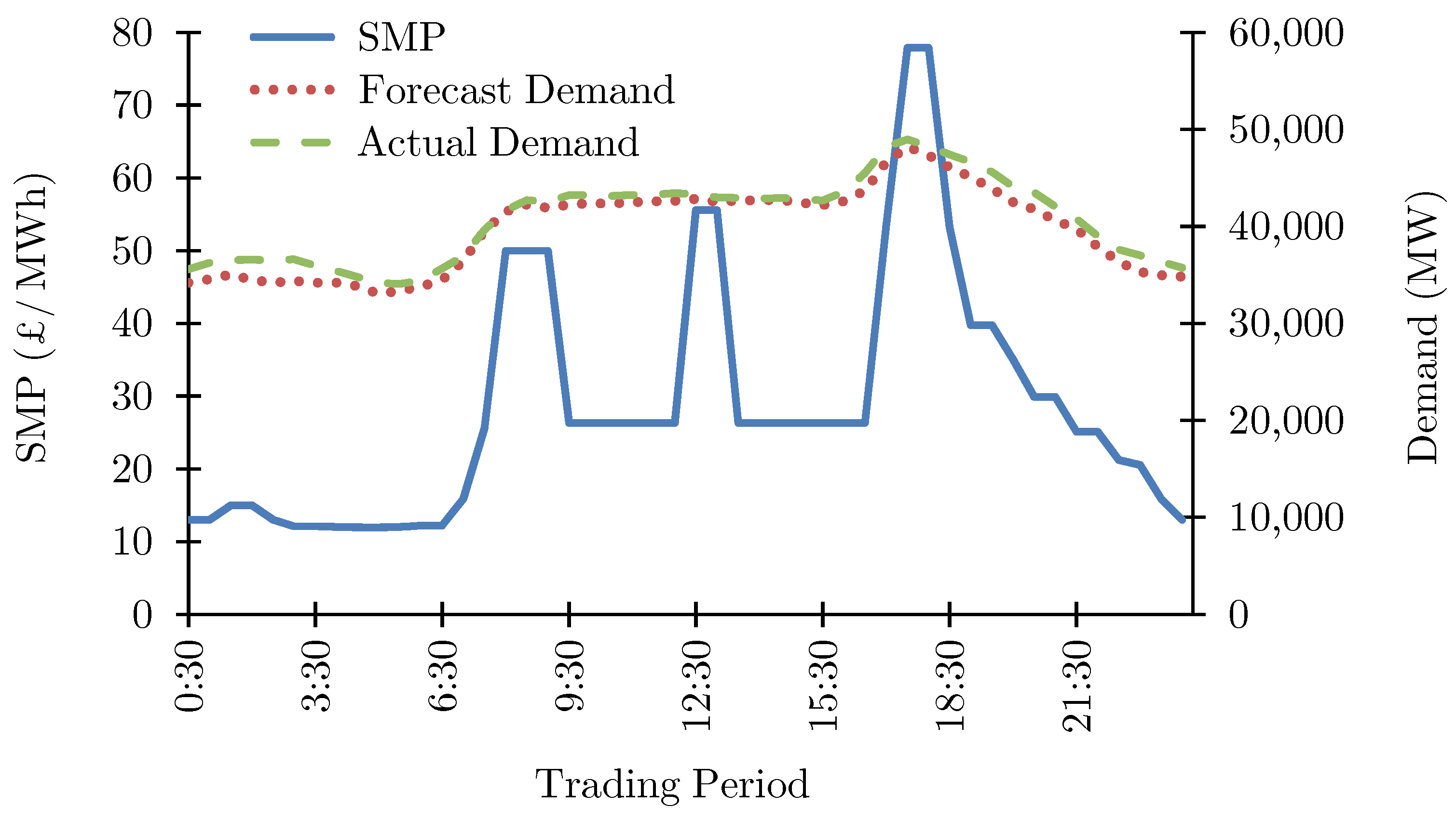
The first data set covers the period from 1 January 1992 to 30 September 2000. This data set includes half-hourly observations on the wholesale electricity price (SMP) and demand for electricity (load). In Figure 5, we provide an illustration of market data for 6 January 2000.
The peak-demand period on this trading day was during 17:30–18:00, when the forecast demand was at the peak of 48,215 MW and SMP is £77.89 per MWh. Changes in forecast demand can be considered as exogenous when analyzing changes in SMP because the forecasting methodology was independent of producers’ bidding.
Figure 6 presents changes and distribution of SMP of the half-hourly peak-demand period over trading days. The empirical distribution (depicted through the histogram) differs substantially from the normal distribution (depicted through the smooth curve). The differences are also confirmed by the calculations of positive skewness, excess kurtosis, and the Jarque–Bera test statistic with its p-value.
In Table 1, we present a detailed analysis of changes in the SMP of the peak-demand period across different regulatory periods summarized in Figure 1. For comparison purposes, we consider the price-cap regulation period (i.e., Regime 3) as the reference period.
For testing the equality of means, we first needed to test the equality of variances using the F-test. The results indicate that, during the price-cap regulation, the average SMP was statistically higher than in the earlier periods (i.e., Regimes 1 and 2). The average SMP rose further after the first series of divestments was introduced (i.e., Regime 4). During Pre-Regime 4 and Regime 5 periods, the average SMP was lower than during the price-cap regulation period.
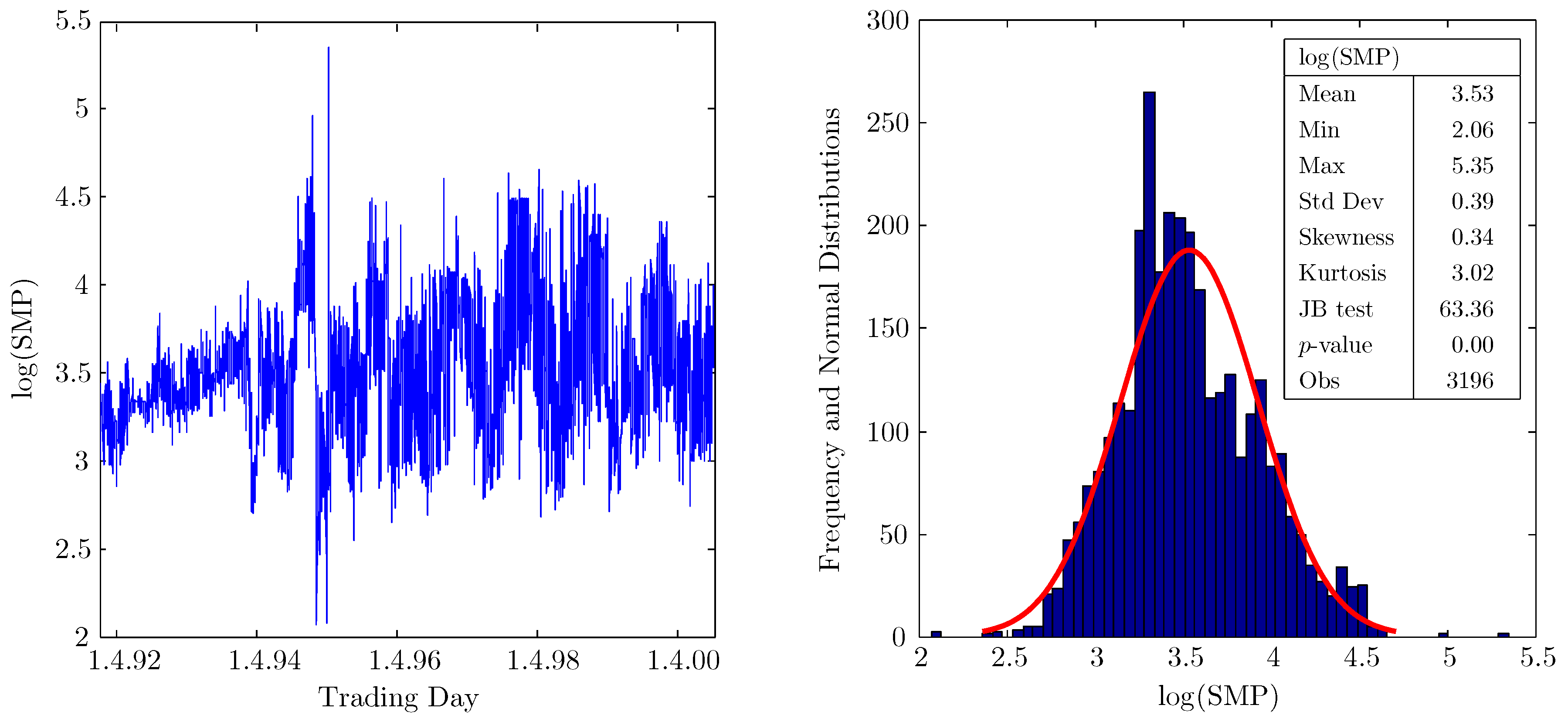
Similar to Figure 6, in Figure 7, we present a log-transformed SMP (i.e., the natural logarithm of SMP), which is used in the empirical part. Using a log transformed time series may help to mitigate the effect of outliers and allow one to interpret regression results in terms of elasticities. (We observe a high SMP of about £211/MWh during the peak-demand period on 4 April 1995. This price spike was brought about by a mistaken mix of technical parameters that the GOAL algorithm had to accept. This explanation is based on a comment from Richard Green.)
The results in the histogram in Figure 7 show that the distribution of log of SMP is skewed to the right and has a peak higher than the peak of normal distribution. Moreover, the result of the Jarque–Bera test rejects the null hypothesis that log of SMP is normally distributed. These issues could be addressed by considering the skew generalized error distribution (SGED) (we do not consider a Student’s t distribution because it assumes a kurtosis below 3), which nests a normal distribution as a special case as shown in Figure 2 and Figure 3.
The second data set covers the period 1 January 1993–30 September 2000 and includes half-hourly data on capacity bids and price bids. Using [3], we can identify production units that were divested from NP and PG during horizontal restructuring, which is important in determining total scheduled capacities of the incumbent producers.
We consider market share as the ratio of total scheduled capacity to forecast demand from the day-ahead bidding data. (The usual interpretation of a market share could be the share of electricity sold on the market, which is not what we consider in this paper.) A firm’s scheduled capacity is based on submitted available capacity of various production units necessary to satisfy forecast demand as described in Figure 4. Market share can be considered as an independent variable when analyzing price changes because SMP was determined after the bidding of producers (i.e., after their submission of price and capacity bids). Sometimes the inclusion of market share may, however, lead to the endogeneity problem. For example, like in the feed-in tariff, when first the electricity price is announced and then the bidding of electricity producers takes place.
In Table 2 and Table 3, we present summary statistics for market shares of the NP and PG producers, which in the early years sometimes served more than 70% of the demand.
Based on the analysis of the coefficient of variation, we find that during almost all regime periods the market share of PG changed more than the market share of NP. However, after the second series of divestments, when on average the market share of NP was lower than the market share of PG, we find that changes in the market share of NP were higher. This could be the result of an unequal horizontal restructuring where NP divested more generation capacity than did PG. Therefore, it is of interest to determine whether, after the divestment series, the effect of incumbent producers’ market shares on SMP remained significant or not.
4. Methodology
In order to analyze the dynamics of SMP during the peak-demand period over trading days we consider the following model:
The first equation is called the mean equation and is analyzed using an autoregressive process with maximum lag order P, that is, . In this equation, the dependent variable is a natural logarithm of SMP (the wholesale price of electricity) during the peak-demand period of trading day t in the day-ahead auction. The process for with selected lags of up to order P allows one to take into account partial adjustment effects and seasonality (cyclical or periodic) features.
Next, in the mean Equation (1), is a vector of explanatory variables including incumbent producers’ market shares, the natural logarithm of forecast demand, and sine and cosine periodic functions. Incumbent producers’ market shares are calculated as a ratio of their total scheduled capacities to forecast demand. The inclusion of market shares is also partly consistent with the methodology in [27], which considers the effect of market concentration measured through the Herfindahl index on Lerner index from April 1996 to September 2002. Interacting the market shares with regime dummy variables should in particular allow for a more detailed analysis of the impact of divestment series on SMP.
Finally, is the disturbance term such that , where represents the information set at time . The disturbance term may be heteroscedastic, which then does not allow for statistical inference about the significance of estimated parameters in the mean equation.
In case the disturbance term has serial correlation or heteroscedasticity problems, one could apply a correction to the standard errors (e.g., Newey–West) or apply the generalized least squares method based on normal distribution (like in [27]). These approaches take into account serial correlation and heteroscedasticity problems in the disturbance term, which then may allow for statistical inference.
Another approach to address the heteroscedasticity problem in the disturbance term could be to consider the autoregressive conditional heteroscedasticity process with maximum lag order p, that is, . This approach was first introduced and applied in [28] to estimate the means and variances of inflation in the UK.
The heteroscedasticity can, therefore, be modeled by the second equation, which is called the volatility equation. Conditional variance and volatility terms (“conditional” is in the sense of conditional on information at time ) are used interchangeably in the literature, which is denoted by , where represents the information set at time . (Volatility can also be rewritten in the following way , where we used .) In this volatility Equation (2), is a vector including regime dummy variables, and sine and cosine periodic functions.
The mean Equation (1) and volatility Equation (2) are jointly called the – model, which we extend by including external regressors. In order to estimate these two equations jointly, a distributional assumption needs to be made for the so-called standardized residuals . The authors in [28] assume that are independent and identically distributed (i.i.d.) and follow a standard normal distribution. In our extended – model, we assume that is independent and identically distributed (i.i.d.) and follows a skew generalized error distribution. This distribution is characterized by four parameters: mean , standard deviation , shape ( corresponds to a leptokurtic distribution with heavy tails and with a peak that is more acute and higher than in a normal distribution), and skewness ( corresponds to a distribution skewed to the right). The skew generalized error distribution is denoted by SGED and described in Figure 2.
Figure 2a describes three special symmetric cases of SGED depending on the value of the shape parameter and the fixed values of , , and : Laplace distribution when , normal distribution when , and uniform distribution when . The symmetric case of the SGED when is known as a generalized error distribution where is a free parameter. (The skewness coefficient and the skewness parameter are not the same concepts. The sample skewness coefficient is a sample statistic, whereas the skewness parameter is the fourth parameter describing the SGED. For a distribution skewed to the right (i.e., with a longer right tail), the skewness coefficient is positive and the skewness parameter is greater than one.)
As described in Figure 2b, in cases of heavy tails and a peak lower than in the normal distribution, a Student’s t distribution could be applicable. However, in the histogram plot in Figure 7, we find that the peak in the distribution of log of SMP is higher than that in the normal distribution. That is why we do not consider a Student’s t distribution. At the same time, though, as the number of degrees of freedom increases, a Student’s t distribution approaches a normal distribution, which is a special case of SGED.
In Figure 3, we schematically illustrate related distributions, where SGED depending on four parameters represents the most flexible and general type of distribution.
In Appendix C, we examine model adequacy by verifying the validity of distributional assumptions of standardized residuals based on the Brock–Dechert–Scheinkman (BDS) test, the Ljung–Box Q-test, skewness and kurtosis measures, kernel density and quantile–quantile plots, and the Jarque–Bera and Kolmogorov–Smirnov normality tests [29,30,31]. Rejecting normality may not mean that the empirical distribution is SGED. That is why we additionally perform the goodness of fit test. Finally, in order to test if the volatility model is correctly specified, we perform the sign bias test developed by [32]. Verifying the validity of distributional assumptions is important in analyzing economic time series with time-varying volatility and for the subsequent interpretation of results.
5. Results
Because stationarity in the time series analysis is a usual requirement in order to allow for modeling and statistical inference, we first provide the results of the stationarity test. We then analyze seasonality properties using the correlogram and periodogram plots. Next, we provide our estimation results for the mean and volatility equations.
5.1. Stationarity Test
We test the stationarity of log of SMP during the half-hourly peak-demand period over trading days using the Augmented Dickey–Fuller (ADF) test with a constant term [33]. This test allows us to control for the possible presence of the serial correlation in the residuals. The maximum lag order is reduced to 21 based on the Schwarz information criterion (SIC). The results of the ADF test are summarized in Table 4.
The unit-root null hypothesis is rejected and therefore we conclude that the log of the SMP time series is stationary. This test result allows us to apply the correlogram and periodogram plots for seasonality analysis, which are presented in the next section.
In Table 5, we similarly present the stationarity test results for the log of the forecast demand time series, which is included as an exogenous variable in modeling the dynamics of the SMP.
The unit-root null hypothesis is rejected, so we conclude that the log of the forecast demand time series is stationary. This test result allows us to apply the Fourier transform in order to construct the periodogram plot for the log of the forecast demand time series. We believe that there may be common frequencies with those of SMP related to seasonality pattern. Including the log of forecast demand may, therefore, lead to a parsimonious model without all frequencies of , , and necessarily being used in sine and cosine periodic functions in order to model the seasonality pattern.
5.2. Seasonality Analysis
In order to analyze seasonality properties and partial adjustment effects on the time domain, we used the autocorrelation function (ACF) and partial autocorrelation function (PACF) plots, respectively. They are summarized in the correlogram presented in Figure 8.
We find that the ACF plot contains spikes at lags of multiples of 7 and 364, which reflect the weekly and annual seasonality patterns in SMP, respectively. These results are empirically important not only for our specification of the process but also for the analysis of firm level data in general including other energy markets. For example, Ref. [34] in the analysis of firm level data of the California electricity market allows for heteroscedasticity and serial correlation in the shocks by computing Newey–West standard errors with a 7-day-lag moving-average structure. The authors in [35,36] in the analysis of market power in the England and Wales wholesale electricity market apply producer–production unit–day of the week clustered standard errors, where the day of the week component allows one to take into account the weekly seasonality pattern, which we also find in this research.
Fourier transform (FT) allows for the analysis of seasonality patterns on the frequency domain. Fourier transform of a real-valued function on the domain is defined as , where i is the imaginary unit such that . Based on this definition, the numerical procedure computes , where , , and N determines the grid. The expressions in parentheses represent scalar products, which in statistical terms measure the covariation between the price time series and the cosine or sine functions for different values of frequency . The optimization finds such values of that would explain a large portion of variation in prices. A graph where the absolute values of the Fourier transform are plotted on the frequency domain is known as a periodogram. The frequencies where the absolute values of Fourier transform achieve local maxima could be used in sine and cosine functions in order to explain seasonal variation in the data.
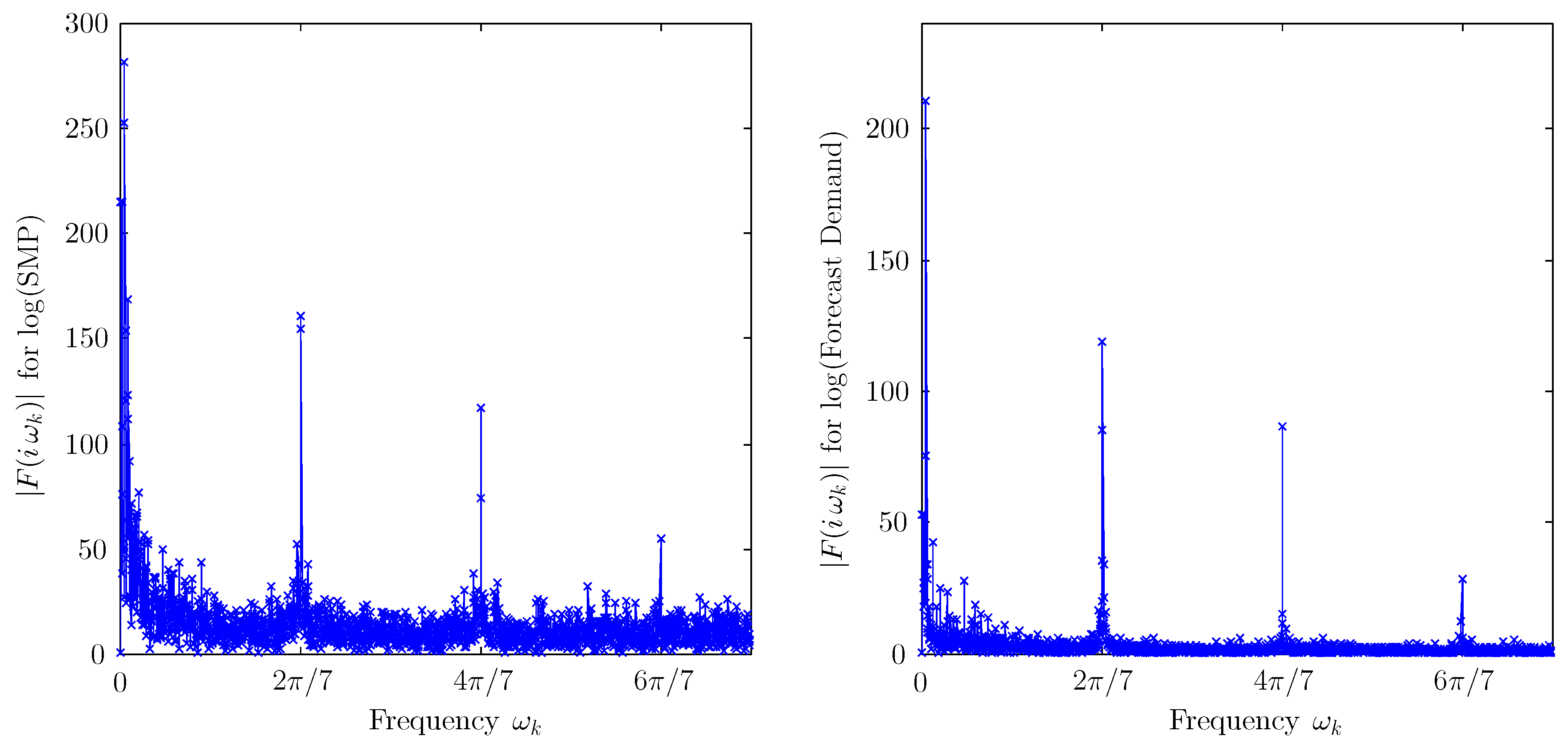
In Figure 9, we summarize in periodogram plots the results of the absolute values of Fourier transform for the log of the SMP and the log of the forecast demand time series.
The periodogram plot suggests using , , and as frequencies for the sine and cosine periodic functions. These periodic functions could incorporate the fact that the behavior of market participants may partly be similar over weeks (for example, one Monday being partly similar to the previous Monday in terms of people’s or the production sector’s electricity consumption pattern).
However, the disadvantage of the Fourier transform is that it does not tell us directly which functions should be used with these identified frequencies: only sine, only cosine, or both. For this purpose, we look at correlations presented in Table 6.
The correlation analysis presented in Table 6 suggests that variable should not be included because correlation between this variable and the dependent variable log (SMP) is not statistically significant.
5.3. Estimation of the Mean and Volatility Equations
Based on the detailed analysis of the correlogram and periodogram plots, we specify the lag structure and frequencies for the sine and cosine functions in the mean and volatility equations. The results presented in Table 7 and Table 8 include standard errors of parameter estimates based on maximum likelihood estimation. These standard errors are correct because all distributional assumptions for are satisfied. In particular, in Appendix C, we test in detail the distributional assumptions for of being i.i.d. and following SGED. The test results confirm the validity of our distributional assumptions.
In Table 7, we provide our estimation results for the mean equation, which includes lags of the dependent variable and exogenous variables (market shares interacted with regime dummy variables, periodic functions, and forecast demand).
The price-cap regulation period (i.e., Regime 3 described in Figure 1) is considered as a reference period. The interaction terms between the regime dummy variables and market shares of incumbent producers allow one to analyze changes in the effect of the incumbents’ market shares on SMP.
Changes in the effect of market shares on SMP are statistically significant before the price-cap regulation period. However, these changes are mostly statistically insignificant after the divestment series is introduced.
The estimation results for the volatility equation, including regime dummy variables and periodic functions as exogenous variables, are presented in Table 8.
Again the price-cap regulation period is considered as a reference period. Coefficient estimates in front of regime dummy variables represent estimates of changes in the intercept term during the other regime periods. These estimates are all statistically significant except for the Pre-Regime 4 period. Interestingly, we find that the second series of divestments was more successful in terms of reduced price volatility since the negative change in the intercept term is also statistically significant.
In estimating the volatility equation, we allow for volatility asymmetry. In other words, we allow for the asymmetric effects of past positive and negative shocks on volatility following [37]. In this approach, measures the direct effect of past shock , and captures the additional effect of negative shock (i.e., in case ) on volatility.
The sum of coefficients in front of the lagged terms in the mean equation is 0.8 and in front of the terms in the volatility equation is 0.5. This is consistent with the stability requirement of being less than 1. Moreover, the positivity of the coefficients of terms and the intercept term in the volatility equation guarantees positivity of conditional volatility.
The estimates of the shape and skewness parameters of SGED suggest that the empirical distribution of standardized residuals has higher kurtosis than in the case of normal distribution (because the estimated shape parameter is statistically lower than 2) and is skewed to the right (because the estimated skewness parameter is statistically greater than 1). If the kurtosis coefficient is equal to 3 (i.e., the shape parameter ) and the skewness coefficient is equal to 0 (i.e., skewness parameter ), then the SGED narrows down to the special case of normal distribution (see Figure 2b). The results are summarized in Table 8 and Table A7.
6. Discussion
In the specification of the mean and volatility equations, we consider the price-cap regulation period (i.e., Regime 3) as a reference period. In the mean equation, in particular, coefficient estimates in front of regime dummy variables interacted with market share reflect changes in the effect of market share on SMP in comparison to the reference period. This approach allows us to understand if, compared to the price-cap regulation period, the observed changes in the effect of market share on SMP during the other regime periods are economically and statistically significant.
In the mean equation, the incumbent producers’ market shares represent an important factor for the policy analysis of the impact of divestment series. As summarized in Table 7, changes in the slope coefficient of market shares for both incumbent producers are statistically significant before price-cap regulation, but are mostly statistically insignificant after the divestment series.
The finding that changes in the effect of market shares are statistically insignificant may not mean that the effect of market shares on SMP after the divestment series is also statistically insignificant. We need to test the significance of the effect of market shares for each regime period separately. Since Regime 3 in Table 7 represents the reference period, first we calculate for the other regime periods, the slope coefficient in front of incumbents’ market shares by adding the coefficient value during Regime 3 (i.e., coefficient ) and the respective change coefficient (i.e., the coefficient in front of market share interacted with the regime dummy variable). In particular, the slope coefficient of NP’s market share for Regime 1 would be the sum of and , which is approximately 0.0159. These calculations are presented in Table 9.
The dependent variable is the natural logarithm of the SMP and market shares are represented as a number, which is why the estimated slope coefficients in front of market shares in Table 7 and Table 9 can be interpreted in percentages. For example, for Regime 1, when the market share of NP increases by 1%, then we can expect the SMP to increase by 0.0159%. A larger market share associated with a higher SMP is not consistent with competitive bidding and may be the result of capacity withholding. That is, a producer may reduce output from low-cost plants and instead increase output from more expensive plants. This strategy is not consistent with competitive bidding because an equilibrium price will be higher.
Capacity withholding was already raised in the literature for various energy markets [25,35,38,39,40]. When demand is expected to be high, even small decreases in the cheaper available capacity may lead to higher prices because the equilibrium takes place at the steeper part of the aggregate supply schedule.
On the other hand, if a producer behaves competitively by submitting price bids reflecting marginal costs, then this may lead to more of its capacity being scheduled for electricity production and hence a larger market share. At the same time, thanks to competitive bidding, equilibrium price is expected to be lower. Therefore, increased scheduled capacity (i.e., a larger market share) associated with a lower SMP is consistent with competition. We observed this effect, for example, for PG during Regime 2 (a negative estimated coefficient of −0.2202 presented in Table 9.
In order to test if the effect of market shares is statistically significant, we need to calculate the respective t-test values, which requires the knowledge of standard errors. These standard errors are calculated based on the variance-covariance matrix of estimated coefficients. In particular, in order to test if the effect of market share of NP is statistically significant in Regime 1, we test the following null hypothesis: . For this purpose, we calculate the t-test value in the following way:
The results are presented in Table 9. We find that the effect of market shares on SMP is significant during and before price-cap regulation.
After both divestment series, the effect of NP’s market share on the SMP is statistically insignificant. This could be regarded as the structural remedy being effective in mitigating the effect of market share on the SMP for NP. After the second series of divestments, the effect of market share on the SMP for PG is, however, statistically significant.
The two incumbent producers were affected differently by divestment series and the structural remedy was effective only for NP. This could be related to unequal horizontal restructuring where NP divested more of its capacity than did PG. As a result, after the second series of divestments PG’s market share was a bit larger than that of NP (Table 2 and Table 3).
These results of the effect of market shares on SMP during the peak-demand period across trading days are new. In the related literature, there were studies analyzing peak-demand periods. For example, market power analysis in [23,36,41].
We also find that an increase in forecast demand by 1% is associated with higher SMP by about 0.17%. This positive relationship is consistent with the market design presented in Figure 4.
Similar to the calculations in Table 9, we use the results in Table 8 in order to present in Table 10 intercept estimates for different regime periods in the volatility equation. In order to test the significance of the intercept term during Regime 1, we test . Here we again calculate the t-test value in the following way:
The intercept term for each regime period is found to be statistically significant. The results also indicate that, during the price-cap regulation period, volatility was higher than in the previous periods. The authors in [6] also found that price volatility increased during the price-cap regulation period. The authors suggest that the incumbent electricity producers could have been deliberately increasing price volatility in order to enjoy higher risk premia in the contract market. After the second series of divestments, we find that price volatility reduced, which we again attribute to the effectiveness of the structural remedy.
Besides [6], price volatility in this market was analyzed in [13] for the daily average SMP using a generalized error distribution in order to incorporate the features of heavy tails and excess kurtosis. Here, however, we use a more flexible skew generalized error distribution, which reflects the features of not only heavy tails and excess kurtosis but also the asymmetry of distribution. Moreover, we do not use the average SMP as was done in [13]. Instead, we consider SMP during the peak-demand period over trading days. We, however, do not consider fuel prices because they are available as quarterly average prices, which are presented in Figure A3. This approach has not been considered in the earlier research on the England and Wales electricity market.
Our findings do not indicate an absolute advantage of the structural remedy over the behavioral remedy. In particular, we find that, after the first series of divestments, price volatility increased and then reduced after the second series of divestments. On the other hand, the effect of market share is qualitatively similar during the price-cap regulation period and after the second series of divestments is introduced. Nevertheless, the effect of market share on SMP for the previously larger incumbent producer is found to be statistically insignificant after the structural remedy is introduced.
7. Conclusions
This paper analyzes the dynamics of the SMP (the wholesale price) in the England and Wales electricity market in relation to the introduced behavioral remedy (through price-cap regulation) and structural remedy (through the divestment series). For this purpose, we consider an – model, which is extended to include incumbents’ market shares. We consider a skew generalized error distribution (SGED) that takes into account asymmetry, excess kurtosis, and heavy tails. We also conduct several statistical tests in order to verify the relevance of applying this distribution. This is necessary for checking the model adequacy and subsequent interpretation of results.
The effect of market shares on the SMP in relation to a divestment series has not been analyzed before. We find that the effect of incumbent producers’ market shares on SMP is sometimes mutually opposite. On the one hand, a larger market share associated with a higher SMP may be related to the incentive to increase more expensive available capacity at the expense of reducing some cheaper available capacity in order to increase prices. On the other hand, if a firm bids competitively, then it may have a larger market share and tend to decrease the equilibrium price.
When comparing the two kinds of remedies, we find qualitatively similar results in the effect of market share during the price-cap regulation period and after the second series of divestments. Statistically, however, the effect of market share after the divestment series is insignificant for NP. Furthermore, price volatility reduced after the second series of divestments.
We do not find an absolute advantage of the structural remedy over the behavioral remedy because the effect of market share on the SMP for PG is statistically significant after the second series of divestments. This result could be related to the finding that, after the second series of divestments, PG’s market share was larger than that of NP.
Even if the effect of market share on the SMP is statistically significant for PG after the second series of divestments, we would still conclude that the structural remedy is more successful because, during price-cap regulation, the effect of market share of both incumbent producers is statistically significant and price volatility is higher. The regulatory office may also prefer a structural remedy that does not involve monitoring costs, as in the case of the behavioral remedy. Moreover, structural remedies in the form of a divestment series may make the market more competitive [34].
The England and Wales electricity market has served as a model for much of the electricity industry restructuring worldwide [24]. The findings of this paper regarding the impact of behavioral and structural remedies on electricity prices could therefore be of interest to other countries (e.g., Australia, Spain, and the U.S.) that have adopted similar trading arrangements.
Funding
This research was supported by a grant from the CERGE-EI Foundation under a program of the Global Development Network. All the opinions expressed are those of the author and have not been endorsed by CERGE-EI or the GDN.
Acknowledgments
I am very grateful to Gregory Crawford, Richard Green, Andrew Sweeting, the Department for Business, Innovation, and Skills (formerly, the Department of Trade and Industry), the National Grid plc, and the Office of Gas and Electricity Markets for providing access to the data and publication materials.
Conflicts of Interest
The authors declare no conflict of interest.
Abbreviations
The following abbreviations are used in this manuscript:
| ACF | Autocorrelation Function |
| ADF | Augmented Dickey–Fuller |
| AR | Autoregressive |
| ARCH | Autoregressive Conditional Heteroscedasticity |
| BDS | Brock–Dechert–Scheinkman |
| CDF | Cumulative Distribution Function |
| Coef of Var | Coefficient of Variation |
| FT | Fourier Transform |
| GOAL | Generator Ordering and Loading |
| i.i.d.hello hello | independent and identically distributed |
| NGC | National Grid Company |
| NP | National Power |
| Obs | Observations |
| PACF | Partial Autocorrelation Function |
| PG | PowerGen |
| SGED | Skew Generalized Error Distribution |
| SIC | Schwarz Information Criterion |
| SMP | System Marginal Price |
| St Dev | Standard Deviation |
Appendix A. Tables

Table A1.
ADF test for the SMP time series.
| Null hypothesis: the SMP time series has a unit root | |
| Exogenous: constant | |
| Lag length: 13 (Automatic choice based on SIC) | |
| ADF test statistic for the SMP time series | −5.217 |
Note: MacKinnon critical values for the rejection of the hypothesis of a unit root: 1% critical value = −3.432, 5% critical value = −2.862, and 10% critical value = −2.567.
Table A2.
ADF test for the forecast demand time series.
| Null hypothesis: the forecast demand time series has a unit root | |
| Exogenous: constant | |
| Lag length: 28 (Automatic choice based on SIC) | |
| ADF test statistic for forecast demand time series | −3.756 |
Note: MacKinnon critical values for the rejection of the hypothesis of a unit root: 1% critical value = −3.432, 5% critical value = −2.862, and 10% critical value = −2.567.
Table A3.
Correlation of the SMP and the forecast demand with periodic functions.
| Variables | ||||||
|---|---|---|---|---|---|---|
| SMP | −0.17 *** | 0.14 *** | −0.09 *** | 0.10 *** | −0.06 *** | 0.02 *** |
| Forecast demand | −0.43 *** | 0.20 *** | −0.18 *** | 0.19 *** | −0.07 *** | 0.06 *** |
Note: *, **, and *** stand for the 10%, 5%, and 1% significance levels, respectively.
Table A4.
Summary statistics of the SMP during the peak-demand period.
| SMP over Weekdays | SMP over Weekends | |
|---|---|---|
| Mean | 39.41 | 30.32 |
| Min | 10.84 | 7.88 |
| Max | 211.24 | 92.66 |
| St Dev | 17.12 | 10.07 |
| Obs | 2283 | 913 |
Appendix B. Figures
Figure A1.
Correlogram for the SMP time series.

Figure A2.
Periodogram plots for the SMP and the forecast demand time series.


Appendix C. Testing Model Adequacy
The adequacy of the estimated model generally depends on the validity of assumptions made prior to estimation. For the maximum likelihood estimation procedure applied in our research, we assume that standardized residuals are independent and identically distributed (i.i.d.) and follow a skew generalized error distribution (SGED). These assumptions are tested and discussed in Appendix C.1 and Appendix C.2, respectively. Finally, in Appendix C.3, using the sign bias test, we examine if in the volatility process there are any asymmetric effects of positive and negative shocks left.
Appendix C.1. Testing the i.i.d. Assumption for the Standardized Residuals
We verify the i.i.d. assumption for the standardized residuals by using two approaches: the Brock–Dechert–Scheinkman (BDS) test and the Ljung–Box Q-test [29,30]. These tests allow one to determine whether there is any information left in standardized residuals .
As summarized in Table A5, for different values of the embedding dimension m and a default option of the proximity parameter , we do not reject the null hypothesis that is i.i.d. time series.
Table A5.
BDS test for .
| Dimension | BDS Stat | Std Err | p-Value |
|---|---|---|---|
| 2 | −0.0006 | 0.0014 | 0.6798 |
| 3 | −0.0004 | 0.0022 | 0.8411 |
| 4 | −0.0001 | 0.0026 | 0.9802 |
| 5 | −0.0005 | 0.0027 | 0.8598 |
| 6 | −0.0007 | 0.0026 | 0.7897 |
Because the above conclusion is based on the parameters of m and , to check robustness, we additionally use the Ljung–Box Q-test. The Q-test allows one to verify if and are serially correlated. Serial correlation in is interpreted as an autocorrelation problem in and serial correlation in is interpreted as a heteroscedasticity problem in . The results of the Ljung–Box Q-test for and are presented in Table A6.
Table A6.
The Ljung–Box Q-test for and .
| Lag | ||||||||
|---|---|---|---|---|---|---|---|---|
| ACF | PACF | Q-Stat | p-Value | ACF | PACF | Q-Stat | p-Value | |
| 1 | −0.01 | −0.01 | 0.44 | 0.51 | −0.02 | −0.02 | 0.94 | 0.33 |
| 5 | 0.03 | 0.03 | 6.77 | 0.24 | 0.00 | 0.00 | 1.49 | 0.91 |
| 10 | −0.01 | −0.01 | 8.17 | 0.61 | 0.03 | 0.03 | 7.83 | 0.65 |
| 50 | 0.01 | 0.01 | 41.18 | 0.81 | 0.01 | 0.00 | 47.12 | 0.59 |
| 100 | −0.02 | −0.01 | 106.40 | 0.31 | 0.04 | 0.04 | 98.69 | 0.52 |
| 200 | −0.01 | −0.01 | 198.74 | 0.51 | 0.00 | 0.01 | 189.73 | 0.69 |
| 300 | 0.01 | 0.01 | 316.63 | 0.24 | 0.00 | 0.02 | 297.89 | 0.52 |
As all p-values from the Ljung–Box Q-test are above 10%, we do not reject the null hypothesis and conclude that time series and are not serially correlated.
Appendix C.2. Testing the Distributional Assumption for the Standardized Residuals
The distributional assumption for the standardized residuals is examined in three steps. In the first step, we analyze descriptive statistics. We then use the Jarque–Bera normality test, the Kolmogorov–Smirnov test, and the quantile–quantile plot in order to compare the empirical distribution with normal distribution. Finally, in the third step, we test if the standardized residuals follow an SGED using the goodness of fit test.
We find that the empirical distribution of standardized residuals has excess kurtosis and heavy tails (a kurtosis coefficient greater than 3 and a shape parameter less than 2). The empirical distribution of is also skewed to the right (a skewness coefficient greater than 0 and a skewness parameter greater than 1). Based on standard errors of and presented in Table 8, we also find that estimated shape and skewness parameters are statistically different from 2 and 1, respectively. These findings are not in line with normal or Student’s t distributions. The results are summarized in Table A7 and Figure A4.
Table A7.
Descriptive statistics for standardized residuals .
| Mean () | −0.0233 |
| Standard deviation () | 1.0022 |
| Kurtosis coefficient | 4.7464 |
| Shape parameter () | 1.4680 |
| Skewness coefficient | 0.2316 |
| Skewness parameter () | 1.0542 |
The Jarque–Bera test allows one to test if the observed excess kurtosis and positive skewness of standardized residuals are jointly statistically significant in order to conclude that the empirical distribution of standardized residuals is different from normal distribution. The results of the Jarque–Bera test presented in Table A8 suggest that the null hypothesis of normal distribution be rejected.
Another way to test if data follow some theoretical distribution (not necessarily normal distribution as was in Jarque–Bera test) is to apply the Kolmogorov–Smirnov test. The idea of this test is based on comparing the differences in cumulative distribution functions (CDF) of empirical and theoretical distributions. We compare the CDFs of empirical and normal distributions. Again we reject the null hypothesis stating that the empirical distribution of standardized residuals is normal at the 5% significance level. In other words, the differences observed between the empirical and normal distributions in Figure A4 are statistically significant. Following the density plots in Figure A4, we suggest that the major reason for rejecting the null hypothesis could be related to excess kurtosis (i.e., kurtosis coefficient greater than 3), heavy tails, and asymmetry observed in the empirical distribution of standardized residuals.
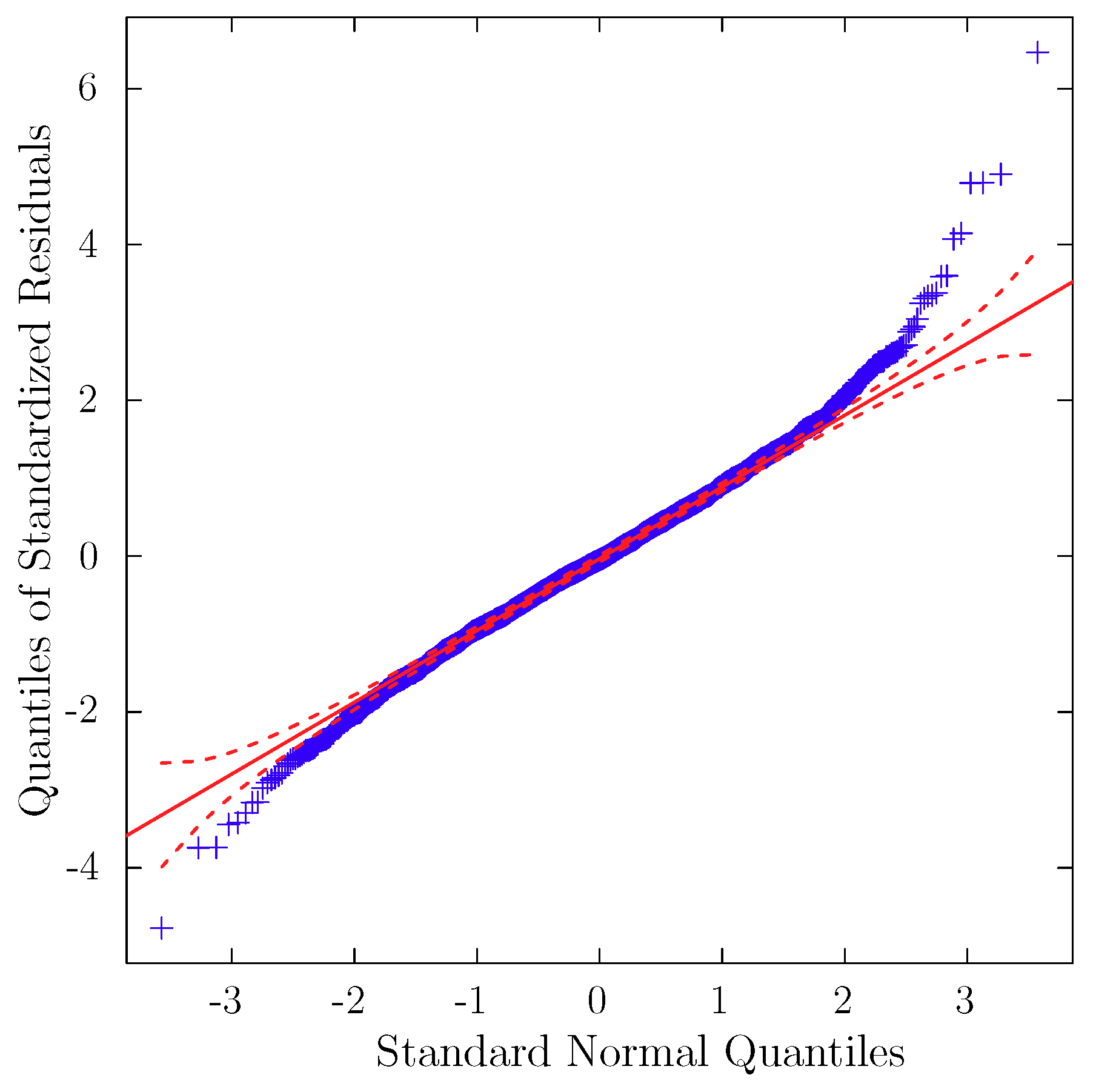
Indeed, when comparing the CDF of the empirical distribution of standardized residuals and normal CDF in Figure A4, we note some differences in tails. The quantile–quantile plot in Figure A5 illustrates more clearly observations in the tails located outside the 95% confidence interval when comparing the empirical and normal distributions.
Figure A4.
The empirical and normal distributions of standardized residuals. (a) Density plots; (b) CDF plots.
Figure A4.
The empirical and normal distributions of standardized residuals. (a) Density plots; (b) CDF plots.

Table A8.
Normality tests for standardized residuals .
| Jarque–Bera Test | Kolmogorov–Smirnov Test | ||
|---|---|---|---|
| Jarque–Bera test statistic | 384.946 | Kolmogorov–Smirnov test statistic | 0.0270 |
| p-value | 0 | p-value | 0.0319 |
Figure A5.
Quantile–quantile plot for standardized residuals.

The finding that the standardized residuals do not follow normal distribution may not necessarily mean that the standardized residuals follow an SGED, even if the SGED nests a normal distribution as a special case. In order to test if the standardized residuals follow an SGED, we apply the goodness of fit test.
In the goodness of fit test, an important parameter is the number of bins (i.e., groups and intervals). Since there are several empirical rules as to how to set the number of bins, we consider four possibilities for the number of bins. The test results in Table A9 suggest not rejecting the null hypothesis, stating that the empirical distribution is the same as the theoretical distribution (i.e., the SGED in our case).
Table A9.
Pearson goodness of fit test.
| Group | -Stat | p-Value |
|---|---|---|
| 20 | 25.28 | 0.15 |
| 30 | 33.42 | 0.26 |
| 40 | 48.50 | 0.14 |
| 50 | 54.24 | 0.28 |
These test results, therefore, support the application of an SGED. This distribution coincides with the normal distribution when the shape parameter is two (i.e., the kurtosis coefficient is three) and the skewness parameter is one (i.e., the skewness coefficient is zero), as illustrated in Figure 2b.
Appendix C.3. Testing Model Specification
The asymmetry of the positive and negative shock effects on volatility was addressed in our methodology following the approach in [37] by introducing parameter in the volatility equation. The presence of remaining asymmetries in the effect of positive and negative shocks on volatility would indicate that the model is misspecified. Hence, we use the sign bias test developed in [32] in order to test the null hypothesis, stating that the conditional volatility model is correctly specified.
Table A10.
Sign bias test.
| t-Test | p-Value | |
|---|---|---|
| Sign bias | 0.25 | 0.81 |
| Negative sign bias | 0.20 | 0.84 |
| Positive sign bias | 0.87 | 0.38 |
| Joint effect | 0.82 | 0.84 |
The test results indicate not rejecting the null hypothesis since all p-values are above 10%. This conclusion suggests that our conditional volatility model has been correctly specified.
References
- Moreno, B.; López, A.J.; García-Álvarez, M.T. The electricity prices in the European Union. The role of renewable energies and regulatory electric market reforms. Energy 2012, 48, 307–313. [Google Scholar] [CrossRef]
- Department of Trade and Industry. Digest of United Kingdom Energy Statistics; Department of Trade and Industry: London, UK, 1997–2002.
- National Grid Company. Seven Year Statement; National Grid Company: Coventry, UK, 1994–2001.
- Newbery, D.M. The UK experience: Privatization with market power. In A European Market for Electricity? Bergman, L., Brunekreeft, G., Doyle, C., von der Fehr, N.H.M., Newbery, D.M., Pollitt, M., Régibeau, P., Eds.; Monitoring European Deregulation; Center for Economic Policy Research: London, UK, 1999; Volume 2, pp. 89–115. [Google Scholar]
- Newbery, D.M. Electricity liberalisation in Britain: The quest for a satisfactory wholesale market design. Energy J. 2005, 26, 43–70. [Google Scholar] [CrossRef]
- Robinson, T.; Baniak, A. The volatility of prices in the English and Welsh electricity pool. Appl. Econ. 2002, 34, 1487–1495. [Google Scholar] [CrossRef]
- Wolfram, C.D. Measuring duopoly power in the British electricity spot market. Am. Econ. Rev. 1999, 89, 805–826. [Google Scholar] [CrossRef]
- Hellström, P.; Maier-Rigaud, F.; Bulst, F.W. Remedies in European antitrust law. Antitrust Law J. 2009, 76, 43–63. [Google Scholar]
- Alexiadis, P.; Sependa, E. Structural remedies under European Union antitrust rules. Compet. Law J. 2013, 21–26. [Google Scholar]
- Chauve, P.; Godfried, M.; Kovács, K.; Nagy, G.L.K.; Siebert, S. The E.ON electricity cases: An antitrust decision with structural remedies. Compet. Policy Newsl. 2009, 51–54. [Google Scholar]
- Maier-Rigaud, F.P. Behavioral versus structural remedies in EU competition law. In European Competition Law Annual 2013, Effective and Legitimate Enforcement of Competition Law; Lowe, P., Marquis, M., Monti, G., Eds.; Hart Publishing: Oxford, UK, 2016; pp. 207–224. [Google Scholar]
- Council Regulation. Council Regulation (EC) No 1/2003 of 16 December 2002 on the implementation of the rules on competition laid down in Articles 81 and 82 of the Treaty. Off. J. Eur. Commun. 2003, L1, 1–25. [Google Scholar]
- Tashpulatov, S.N. Estimating the volatility of electricity prices: The case of the England and Wales wholesale electricity market. Energy Policy 2013, 60, 81–90. [Google Scholar] [CrossRef]
- Koopman, S.J.; Ooms, M.; Carnero, M.A. Periodic seasonal Reg-ARFIMA-GARCH models for daily electricity spot prices. J. Am. Stat. Assoc. 2007, 102, 16–27. [Google Scholar] [CrossRef]
- Frömmel, M.; Han, X.; Kratochvil, S. Modeling the daily electricity price volatility with realized measures. Energy Econ. 2014, 44, 492–502. [Google Scholar] [CrossRef]
- Borenstein, S.; Bushnell, J.B.; Wolak, F.A. Measuring market inefficiencies in California’s restructured wholesale electricity market. Am. Econ. Rev. 2002, 92, 1376–1405. [Google Scholar] [CrossRef]
- Cramton, P.; Stoft, S. Why we need to stick with uniform-price auctions in electricity markets. Electr. J. 2007, 20, 26–37. [Google Scholar] [CrossRef]
- Green, R.J. Failing electricity markets: Should we shoot the pools? Util. Policy 2003, 11, 155–167. [Google Scholar] [CrossRef]
- Bergman, L.; Doyle, C.; Gual, J.; Hultkrantz, L.; Neven, D.; Röller, L.H.; Waverman, L. Europe’s Network Industries: Conflicting Priorities—Telecommunications; Monitoring European Deregulation; Center for Economic Policy Research: London, UK, 1998; Volume 1. [Google Scholar]
- Joskow, P.L. Lessons learned from electricity market liberalization. Energy J. 2008, 29, 9–42. [Google Scholar] [CrossRef]
- Joskow, P.L. Foreword: US vs. EU electricity reforms achievement. In Electricity Reform in Europe; Glachant, J.M., Lévêque, F., Eds.; Edward Elgar Publishing Limited: Cheltenham, UK, 2009; pp. xiii–xxix. [Google Scholar]
- Electricity Pool. Pooling and Settlement Agreement for the Electricity Industry in England and Wales; Electricity Pool of England and Wales: London, UK, 1999. [Google Scholar]
- Sweeting, A. Market power in the England and Wales wholesale electricity market 1995–2000. Econ. J. 2007, 117, 654–685. [Google Scholar] [CrossRef]
- Wolak, F.A. Market design and price behavior in restructured electricity markets: An international comparison. In Deregulation and Interdependence in the Asia-Pacific Region; NBER-EASE; Springer: Boston, MA, USA, 2000; Volume 8, pp. 79–137. [Google Scholar]
- Wolak, F.A.; Patrick, R.H. The Impact of Market Rules and Market Structure on the Price Determination Process in the England and Wales Electricity Market; NBER Working Paper Series No. 8248; National Bureau of Economic Research: Cambridge, MA, USA, 2001; pp. 1–86. [Google Scholar]
- Green, R.J. Market power mitigation in the UK power market. Util. Policy 2006, 14, 76–89. [Google Scholar] [CrossRef] [Green Version]
- Evans, J.E.; Green, R.J. Why Did British Electricity Prices Fall after 1998? Cambridge Working Papers in Economics CWPE 0326; University of Cambridge: Cambridge, UK, 2003. [Google Scholar]
- Engle, R.F. Autoregressive conditional heteroscedasticity with estimates of the variance of United Kingdom inflation. Econometrica 1982, 50, 987–1007. [Google Scholar] [CrossRef]
- Brock, W.A.; Dechert, W.D.; Scheinkman, J.A.; LeBaron, B. A test for independence based on the correlation dimension. Econ. Rev. 1996, 15, 197–235. [Google Scholar] [CrossRef]
- Ljung, G.M.; Box, G.E.P. On a measure of lack of fit in time series models. Biometrika 1978, 65, 297–303. [Google Scholar] [CrossRef] [Green Version]
- Hazewinkel, M. (Ed.) Encyclopaedia of Mathematics; Kluwer Academic Publishers: Dordrecht, The Netherlands, 1990; Volume 5. [Google Scholar]
- Engle, R.F.; Ng, V.K. Measuring and testing the impact of news on volatility. J. Financ. 1993, 48, 1749–1777. [Google Scholar] [CrossRef]
- Dickey, D.A.; Fuller, W.A. Likelihood ratio statistics for autoregressive time series with a unit root. Econometrica 1981, 49, 1057–1072. [Google Scholar] [CrossRef]
- Puller, S.L. Pricing and firm conduct in California’s deregulated electricity market. Rev. Econ. Stat. 2007, 89, 75–87. [Google Scholar] [CrossRef]
- Lízal, L.M.; Tashpulatov, S.N. Do producers apply a capacity cutting strategy to increase prices? The case of the England and Wales electricity market. Energy Econ. 2014, 43, 114–124. [Google Scholar] [CrossRef]
- Tashpulatov, S.N. Analysis of electricity industry liberalization in Great Britain: How did the bidding behavior of electricity producers change? Util. Policy 2015, 36, 24–34. [Google Scholar] [CrossRef]
- Glosten, L.R.; Jagannathan, R.; Runkle, D.E. On the relation between the expected value and the volatility of the nominal excess returns on stocks. J. Financ. 1993, 48, 1779–1801. [Google Scholar] [CrossRef]
- Dechenaux, E.; Kovenock, D. Tacit collusion and capacity withholding in repeated uniform price auctions. RAND J. Econ. 2007, 38, 1044–1069. [Google Scholar] [CrossRef] [Green Version]
- Fridolfsson, S.O.; Tangerås, T.P. Market power in the Nordic electricity wholesale market: A survey of the empirical evidence. Energy Policy 2009, 37, 3681–3692. [Google Scholar] [CrossRef]
- Castro-Rodriguez, F.; Marín, P.L.; Siotis, G. Capacity choices in liberalized electricity markets. Energy Policy 2009, 37, 2574–2581. [Google Scholar] [CrossRef]
- Crawford, G.S.; Crespo, J.; Tauchen, H. Bidding asymmetries in multi-unit auctions: Implications of bid function equilibria in the British spot market for electricity. Int. J. Ind. Organ. 2007, 25, 1233–1268. [Google Scholar] [CrossRef]
- Department of Trade and Industry. Energy Trends; Department of Trade and Industry: London, UK, 1993–2000.

Figure 2.
An SGED and a skew Student’s t distribution. Notes: In (a), we show special cases of the shape parameter , , and which correspond to Laplace (black), Standard Normal (red), and Uniform (green) distributions, respectively. In (b), we include a skew Student’s t distribution with degrees of freedom equal to 8, i.e., . It is skewed to the right because the skewness parameter exceeds 1, i.e., . (a) Special cases of SGED; (b) normal and skew Student’s t distributions.

Figure 3.
All special cases of SGED .

Figure 4.
Determination of a System Marginal Price (SMP). Notes: On the vertical axis, refers to the price bid of electricity producer A’s first production unit, whose production capacity is . For the sake of simplicity, it is assumed that electricity producer A has 2 coal and 3 gas production unit types. Price bids of all production units are ordered as would have been done by the market operator (i.e., the NGC). The intersection of the constructed production schedule and forecast demand determines the SMP, the wholesale electricity price. In this hypothetical example, it is electricity producer A’s third gas production unit that determines the SMP.

Figure 5.
SMP, forecast demand, and actual demand (6 January 2000).

Figure 6.
SMP during the peak-demand period over trading days (1 January 1992–30 September 2000).

Figure 7.
Log of SMP during the peak-demand period over trading days (1 January 1992– 30 September 2000).
Figure 7.
Log of SMP during the peak-demand period over trading days (1 January 1992– 30 September 2000).

Figure 8.
Correlogram for the log of the SMP time series.

Figure 9.
Periodogram plots for the log of the SMP and the log of the forecast demand time series.

Table 1.
Summary statistics for SMP (£/MWh) during the peak-demand period over trading days.
| SMP | Regime 1 (Jan 92 –Mar 93) | Regime 2 (Apr 93 –Mar 94) | Regime 3 (Apr 94 –Mar 96) Price-Cap | Pre-Regime 4 (Apr 96 –Jul 96) | Regime 4 (Jul 96 –Jul 99) Divestment 1 | Regime 5 (Jul 99 –Sept 00) Divestment 2 |
|---|---|---|---|---|---|---|
| Mean | 27.5 | 32.9 | 37.2 | 35.3 | 42.0 | 36.3 |
| Change of Mean | −9.7 | −4.3 | −2.0 | 4.8 | −0.9 | |
| t-test | −14.4 | −5.9 | −1.4 | 5.5 | −1.1 | |
| t-critical | −2.0 | −2.0 | −2.0 | 2.0 | −2.0 | |
| Min | 17.3 | 14.9 | 7.9 | 17.2 | 14.5 | 15.5 |
| Max | 46.2 | 55.9 | 211.2 | 76.7 | 105.1 | 77.9 |
| St Dev | 3.7 | 6.5 | 17.6 | 11.4 | 19.3 | 12.1 |
| F-test | 23.0 | 7.3 | 2.4 | 1.2 | 2.1 | |
| F-critical | 1.2 | 1.2 | 1.3 | 1.1 | 1.2 | |
| Coef of Var (%) | 13.4 | 19.8 | 47.4 | 32.3 | 45.9 | 33.5 |
| Obs | 456 | 365 | 731 | 91 | 1114 | 439 |
Table 2.
Summary statistics for NP’s market share during the peak-demand period over trading days.
| Regime 1 (Jan 93 –Mar 93) | Regime 2 (Apr 93 –Mar 94) | Regime 3 (Apr 94 –Mar 96) Price-Cap | Pre-Regime 4 (Apr 96 –Jul 96) | Regime 4 (Jul 96 –Jul 99) Divestment 1 | Regime 5 (Jul 99 –Sept 00) Divestment 2 | |
|---|---|---|---|---|---|---|
| Mean | 0.449 | 0.426 | 0.367 | 0.297 | 0.229 | 0.124 |
| Min | 0.341 | 0.286 | 0.165 | 0.227 | 0.086 | 0.062 |
| Max | 0.506 | 0.503 | 0.501 | 0.350 | 0.317 | 0.181 |
| St Dev | 0.037 | 0.038 | 0.047 | 0.028 | 0.034 | 0.022 |
| Coef of Var (%) | 8.21 | 8.93 | 12.68 | 9.44 | 14.98 | 17.96 |
| Obs | 90 | 365 | 731 | 91 | 1114 | 439 |
Table 3.
Summary statistics for PG’s market share during the peak-demand period over trading days.
| Regime 1 (Jan 93 –Mar 93) | Regime 2 (Apr 93 –Mar 94) | Regime 3 (Apr 94 –Mar 96) Price-Cap | Pre-Regime 4 (Apr 96 –Jul 96) | Regime 4 (Jul 96 –Jul 99) Divestment 1 | Regime 5 (Jul 99 –Sept 00) Divestment 2 | |
|---|---|---|---|---|---|---|
| Mean | 0.278 | 0.247 | 0.245 | 0.230 | 0.202 | 0.141 |
| Min | 0.219 | 0.128 | 0.123 | 0.166 | 0.096 | 0.069 |
| Max | 0.346 | 0.318 | 0.331 | 0.277 | 0.284 | 0.193 |
| St Dev | 0.033 | 0.035 | 0.035 | 0.025 | 0.028 | 0.017 |
| Coef of Var (%) | 11.98 | 14.06 | 14.21 | 10.84 | 13.97 | 11.99 |
| Obs | 90 | 365 | 731 | 91 | 1114 | 439 |
Table 4.
The ADF test for the log of the SMP time series.
| Null hypothesis: the log of the SMP time series has a unit root | |
| Exogenous: constant | |
| Lag length: 21 (Automatic based on SIC) | |
| ADF test statistic for the log of the SMP time series | −5.349 |
Note: MacKinnon critical values for the rejection of the hypothesis of a unit root: 1% critical value = −3.432, 5% critical value = −2.862, and 10% critical value = −2.567.
Table 5.
ADF test for the log of the forecast demand time series.
| Null hypothesis: the log of the forecast demand time series has a unit root | |
| Exogenous: constant | |
| Lag length: 28 (Automatic based on SIC) | |
| ADF test statistic for the log of the forecast demand time series | −3.650 |
Note: MacKinnon critical values for the rejection of the hypothesis of a unit root: 1% critical value = −3.432, 5% critical value = −2.862, and 10% critical value = −2.567.
Table 6.
Correlation of the log of the SMP and the log of the forecast demand with periodic functions.
Table 6.
Correlation of the log of the SMP and the log of the forecast demand with periodic functions.
| Variable | ||||||
|---|---|---|---|---|---|---|
| log(SMP) | −0.18 *** | 0.14 *** | −0.10 *** | 0.10 *** | −0.06 *** | 0.02 *** |
| log(Forecast demand) | −0.44 *** | 0.20 *** | −0.19 *** | 0.19 *** | −0.07 *** | 0.07 *** |
Note: *, **, and *** stand for the 10%, 5%, and 1% significance levels, respectively.
Table 7.
Mean equation .
| Intercept Term and | Coef | Std Err | Exogenous Variables | Coef | Std Err |
|---|---|---|---|---|---|
| Lagged Terms | a | a | |||
| −1.09005 *** | 0.00290 | 0.03584 *** | 0.00011 | ||
| 0.30204 *** | 0.00073 | 0.28354 *** | 0.05289 | ||
| 0.11736 *** | 0.00031 | −0.01995 *** | 0.00007 | ||
| 0.06675 *** | 0.00017 | 0.90364 | 0.60383 | ||
| 0.06126 *** | 0.00016 | 0.26883 ** | 0.14972 | ||
| 0.12551 *** | 0.00035 | −0.59855 | 0.38660 | ||
| 0.19530 *** | 0.00049 | −0.28930 *** | 0.00078 | ||
| −0.09317 *** | 0.00024 | −0.52879 *** | 0.08924 | ||
| −0.05304 *** | 0.00014 | 0.30861 *** | 0.00083 | ||
| 0.11632 *** | 0.00031 | −1.08304 | 0.77633 | ||
| 0.09109 *** | 0.00023 | −0.17788 | 0.17213 | ||
| −0.05007 *** | 0.00013 | 0.54115 | 0.33167 | ||
| −0.04189 *** | 0.00011 | 0.02114 *** | 0.00007 | ||
| −0.04919 *** | 0.00013 | 0.02690 *** | 0.00008 | ||
| 0.05135 *** | 0.00013 | −0.01248 *** | 0.00004 | ||
| −0.02990 *** | 0.00008 | 0.16719 *** | 0.00031 | ||
| −0.04056 *** | 0.00011 | ||||
| −0.04248 *** | 0.00011 | 0.606 | |||
| 0.06847 *** | 0.00018 | Obs | 2823 |
Notes: The inclusion of some of the lags of the dependent variable helps as a correction for serial correlation in the error term. In the table, and stand for the natural logarithm of the SMP and the forecast demand during the peak-demand period of trading day t (), respectively. The number of included observations is less because of lagged terms. is a vector of exogenous variables including market shares interacted with regime dummy variables, periodic functions, and forecast demand. Standard errors are based on maximum likelihood estimation. *, **, and *** stand for the 10%, 5%, and 1% significance levels, respectively.
Table 8.
Volatility equation .
| Intercept Term and | Coef | Std Err | Exogenous Variables | Coef | Std Err |
|---|---|---|---|---|---|
| ARCH Terms | a | ||||
| 0.03824 *** | 0.00012 | −0.03342 *** | 0.00011 | ||
| 0.09687 *** | 0.00035 | −0.02853 *** | 0.00107 | ||
| 0.07501 *** | 0.00032 | 0.02269 ** | 0.01484 | ||
| 0.04659 *** | 0.00018 | 0.00589 ** | 0.00341 | ||
| 0.05782 *** | 0.00019 | −0.00667 ** | 0.00364 | ||
| 0.07095 *** | 0.00024 | 0.00203 *** | 0.00001 | ||
| 0.00479 *** | 0.00003 | 0.00468 *** | 0.00001 | ||
| 0.15345 *** | 0.00053 | ||||
| 0.04791 *** | 0.00023 | SGED parameters | |||
| Shape parameter, | 1.46803 *** | 0.05237 | |||
| Skewness parameter, | 1.05424 *** | 0.02471 |
Notes: stands for conditional volatility as described in Footnote 4. is an indicator function equal to 1 if and 0 otherwise. is a vector of exogenous variables including regime dummy variables and periodic functions. Standard errors are based on maximum likelihood estimation. *, **, and *** stand for the 10%, 5%, and 1% significance levels, respectively.
Table 9.
The effect of market share of NP and PG on SMP across different regimes.
| Regime 1 (Jan 93–Mar 93) | Regime 2 (Apr 93–Mar 94) | Regime 3 (Apr 94–Mar 96) Price-Cap | Pre-Regime (Apr 96–Jul 96) | Regime 4 (Jul 96–Jul 99) Divestment 1 | Regime 5 (Jul 99–Sept 00) Divestment 2 | |
|---|---|---|---|---|---|---|
| Coef of | 0.0159 | 0.2636 | −0.0200 | 0.8837 | 0.2489 | −0.6185 |
| Std Err | 0.0001 | 0.0529 | 0.0001 | 0.6038 | 0.1497 | 0.3866 |
| t-test | 121.8835 | 4.9836 | −307.3769 | 1.4635 | 1.6623 | −1.5998 |
| t-critical | 2.0 | 2.0 | −2.0 | 2.0 | 2.0 | −2.0 |
| Coef of | 0.0193 | −0.2202 | 0.3086 | −0.7744 | 0.1307 | 0.8498 |
| Std Err | 0.0011 | 0.0892 | 0.0008 | 0.7763 | 0.1721 | 0.3317 |
| t-test | 17.1774 | −2.4672 | 372.2598 | −0.9975 | 0.7594 | 2.5621 |
| t-critical | 2.0 | −2.0 | 2.0 | −2.0 | 2.0 | 2.0 |
| Obs | 90 | 365 | 731 | 91 | 1114 | 439 |
Note: Calculations are based on Table 7.
Table 10.
Volatility across different regimes.
| Regime 1 (Jan 93–Mar 93) | Regime 2 (Apr 93–Mar 94) | Regime 3 (Apr 94–Mar 96) Price-Cap | Pre-Regime (Apr 96–Jul 96) | Regime 4 (Jul 96–Jul 99) Divestment 1 | Regime 5 (Jul 99–Sept 00) Divestment 2 | |
|---|---|---|---|---|---|---|
| Intercept | 0.0048 | 0.0097 | 0.0382 | 0.0609 | 0.0441 | 0.0316 |
| Std Err | 0.0002 | 0.0011 | 0.0001 | 0.0148 | 0.0034 | 0.0036 |
| t-test | 23.8783 | 9.1378 | 321.3917 | 4.1052 | 12.9518 | 8.6768 |
| t-critical | 2.0 | 2.0 | 2.0 | 2.0 | 2.0 | 2.0 |
| Obs | 90 | 365 | 731 | 91 | 1114 | 439 |
Note: Calculations are based on Table 8.
© 2018 by the author. Licensee MDPI, Basel, Switzerland. This article is an open access article distributed under the terms and conditions of the Creative Commons Attribution (CC BY) license (http://creativecommons.org/licenses/by/4.0/).
Share and Cite
MDPI and ACS Style
Tashpulatov, S.N. The Impact of Behavioral and Structural Remedies on Electricity Prices: The Case of the England and Wales Electricity Market. Energies 2018, 11, 3420. https://doi.org/10.3390/en11123420
AMA Style
Tashpulatov SN. The Impact of Behavioral and Structural Remedies on Electricity Prices: The Case of the England and Wales Electricity Market. Energies. 2018; 11(12):3420. https://doi.org/10.3390/en11123420
Chicago/Turabian StyleTashpulatov, Sherzod N. 2018. "The Impact of Behavioral and Structural Remedies on Electricity Prices: The Case of the England and Wales Electricity Market" Energies 11, no. 12: 3420. https://doi.org/10.3390/en11123420
Note that from the first issue of 2016, this journal uses article numbers instead of page numbers. See further details here.