Economic Analysis for Residential Solar PV Systems Based on Different Demand Charge Tariffs

Abstract

It is well known that the use of photovoltaic (PV) systems helps to preserve the environment, produce lower levels of greenhouse gases (GHGs), and reduce global warming, however, whether it is economically profitable for customers or not is highly debatable. This paper aims to address this issue. To be comprehensive, three different types of buildings are considered as case studies. Then, these three buildings are modeled in EnergyPlus to determine the rate of energy consumption. Afterward, comparisons of various solar system sizes based on economic parameters such as the internal rate of return, the net present value, payback period and profitability indexing for various-sized PV systems are carried out. The results show that by the demand charge tariffs, using PV systems has no economic justification. It has been shown that even with neglecting further costs of the PV system like maintenance, by demand charge tariffs, it is not economically beneficial for customers to use the PV systems. Profitability index of all three buildings with various PV power systems is between 0.2 to 0.8, which are by no means is desirable. Moreover, it was found that bigger solar systems are less cost-effective in the presence of demand charges.

1. Introduction

Energy has been one of the most important factors in human progress throughout history. Most energy usage is from non-renewable sources, especially fossil fuels and the consumption of the renewable energy sources is faster than their production speed [1]. Fossil fuels currently supply about 85 percent of the total energy usage worldwide [2]. Evidently, dependence on the fossil fuels will increase greenhouse gas (GHG) emissions, air pollution and global warming, and continuing this process may cause serious natural disasters [3].

For many decades, electricity has been used for various reasons. Electricity is a versatile type of energy that can be easily controlled and transported. This unique feature of electricity has caused the public significantly to rely on it for use in many usual applications. Therefore, electricity consumption has risen every year from 1949 to now, except for 1979 and 1992 [4]. While energy prices have also increased along with the higher demand, available energy sources have fallen [5]. Due to the increasing growth of electric power consumption and its price, many researchers have focused on finding better, cheaper and cleaner ways to generate electricity.

To address these issues, renewable energies as environmentally friendly resources have drawn attention. Renewable or alternative energy is defined as the energy that can be obtained from the sources replenishing themselves such as rivers, geothermal, biofuel, wind, sun and so on [4]. The favorable features of renewable energy have led governments to take steps to make more use of this type of energies. For example, after the oil embargo of 1973, renewable energy, which traditionally was considered to be too expensive and technologically immature, became a strong force in the U.S. scene [4].

One of the most promising renewable energy resources is solar energy. About 1400 J/m²·s energy is radiated to the earth from the sun which is considerably more than the total energy use worldwide [6]. Apart from its abundance, it is a clean and well-distributed energy in the world. The important point is how to harvest this energy in an optimum way.

Photovoltaic (PV) systems, which convert the light of the sun to the electric power, are a common way of using solar energy. PV is the quickest growing energy technology on the planet [7], and annually 50 GW of new capacities are added to the existing installed capacity [8]. PV technology is probably the best type of the renewable energy that can be achieved because it has the minimum destruction effect on the environment [9]. Also, PV has some other promising features, such as avoidance of energy transmission, removing the energy losses due to generating energy in the place of usage, and silent energy production [10].

After the discovery of the PV effect in 1839 by the French physicist Edmond Becquerel [11], researchers focused their attention on increasing the efficiency of solar cells by changing their material. Moreover, apart from the material, it has been shown that decreasing in the panel temperature of PV systems can lead to a significant increase in their efficiency [12]. Another promising progress in increasing the efficiency of the PV systems was carried out by Das et al. [13]. They claimed that utilizing multi-junction solar cells can provide about three times power more than the conventional systems [14]. At the time, the priority of scientists was generating the maximum possible power without considering the financial issues [15]. Later, when the environmental effect and quick depletion of other conventional resources drew attention, the economic issues became more important. However, solar energy is very efficient, but harnessing it is costly. According to Borenstein [4], the cost of solar panels is one of its major drawbacks, preventing it from market anticipation. However, it is worth mentioning, although solar cells prices are still relatively expensive, their prices are declining, and the demand for their use in larger scales is increasing [16].

The building sector is responsible for one-third of the global energy consumption and the same portion of GHG emissions [17]. Since PV systems are reliable, easy to install, have predictable annual yields, and can be used for electric appliances, lighting, heaters, heat pumps, or even charging electric cars, they are known as a promising addition to the existing energy system. Therefore, PV systems are suitable to be used in buildings separately or in a combination with other energies [18].

To utilize the PV systems in a building, it is necessary to evaluate its financial benefits. Bernal-Agustı´n and Dufo-Lo´pez [19] investigated the environmental and economic facets of the grid-connected PV systems by considering the life cycle analysis (LCA) theory. Oliver and Jackson [20] applied economic and energy analysis to evaluate the application of the building integrated PV system. Some other works considering the economic and/or environmental aspects of the PV systems were investigated in the literature [21,22,23,24]. Based on the life cycle cost (LCC), Kolhe et al. [25] examined different mixes of generators and PV systems for an Indian school. They concluded that the use of a stand-alone PV was very suitable when the need for the energy was low and found that it would be more competitive when the PV prices decrease. Ajan et al. [26] studied the feasibility of using an off-grid system which blends the technology of the PV with a diesel generator, in a case study for a school in East Malaysia, Sarawak. Their results showed that because of the high price of the PV systems, it is not beneficial for the school to invest in this type of renewable energy. To generate electricity for a distant household area in Egypt, Nafeh created a stand-alone PV system; its generated electricity was used to supply a single residential building in Sinai Peninsula of Egypt. His proposed design system considers the sun radiation and the typical power consumption of a residential home [27]. Ojosu noted that the PV energy systems could play a substantial role in electrical supplementation of places like Nigeria, which has abundant solar energy resources. He argued that if the price of the PV systems falls down, it is reasonable to use the PV system as the primary source of energy for Nigeria when its average daily solar radiation is between 4 and 6 KW/m²/day [28]. Many other researchers investigated the potential usage of PV systems for different parts of the world like China, Portugal and so forth [29,30,31]. Considering so many investigations, it can be concluded that in many locations in the world energy can be supplied with the help of PV systems.

Although a large number of studies have been done in the field of economic analysis of PV systems, there are still several reasons to justify further research in this topic area. The first reason is that many of the thermal modeling studies have not been done accurately and the basis for the building thermal modeling was a simple relationship, and most of the previous studies did not validate their modeling results by the reliable experimental data [14,15,19]. Secondly, because of continuous change of the electricity tariffs, an updated analysis is required. Lastly, for costumers, it is essential to evaluate the benefits of the PV system from a purely economic perspective. It is evident that using PV systems is good for the environment, but customers need to know if the investments in these systems are indeed profitable.

Recently, some electrical utilities have introduced the demand charge tariffs for the residential customers who decide to install the solar systems. Such new tariffs are actually a move toward the lower energy and higher demand rates. However, many people in the solar industry believe that these price plans would reduce the profitability of residential solar investment. To evaluate these new price plans, this study uses three sample buildings modeled and validated in prior works [32,33]. Such validations are performed as a basis for energy consumption and aim to find the optimum solar system sizes in the presence of the demand charges. Two US states that have introduced demand charges are studied as case studies.

This paper examines the economic benefits of PV systems for various buildings and different price plans. The paper is organized as follows: methodology, which consists of introducing the simulation software, explaining the case studies, and defining price plans. Then, economics parameters are briefly presented. Afterwards, validation of the simulation is described, and later results are clearly explained, answering whether the PV system is beneficial or not, and finally, the conclusions are presented.

2. Methodology

2.1. Simulator Software

In this research, EnergyPlus was used as a simulation tool. This software performs universal modeling of a building envelope, Heating Ventilation and Air Conditioning (HVAC) system, fenestration, and daylighting and can calculate cooling and heating loads, power consumption throughout all hours of the year and a large number of other parameters. EnergyPlus has been expanding since 2003 by adding this module to perform modeling based on the PV systems and solar thermal hot water systems. This change afforded the software to be able to model the zero-energy buildings [34]. The application of EnergyPlus in this study was due to its precise solver engine, free software and matching all of our requirements.

2.2. Case Studies

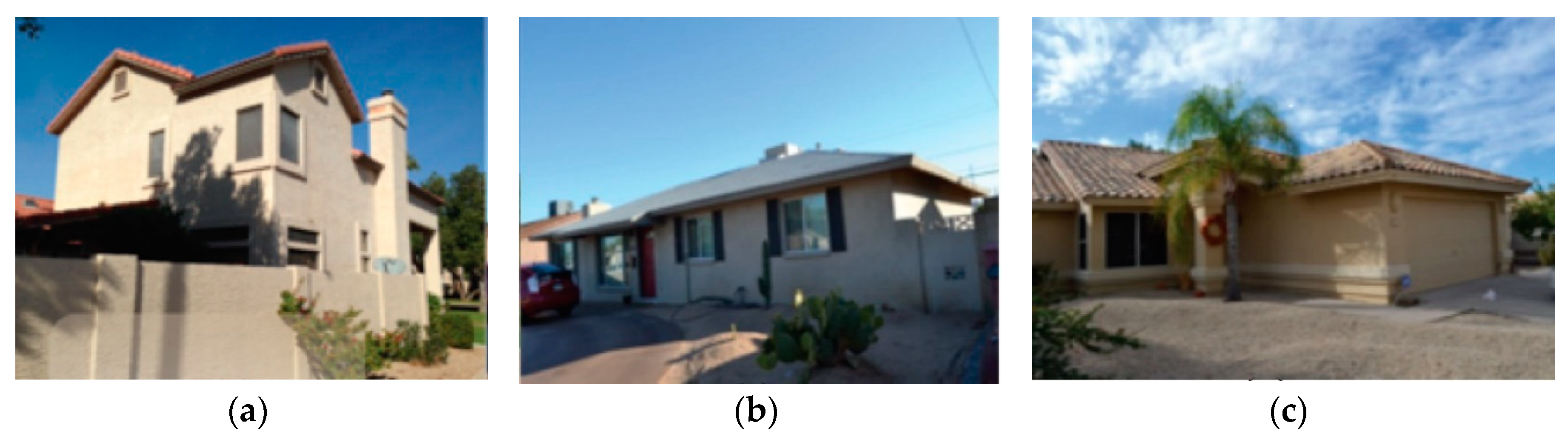
In this research, three different types of residential buildings are considered as sample buildings representing the residential building stock in the two states. The simulation work is done for different buildings to represent the majority of the residential buildings. As shown in Figure 1, the first one is a two-story house with wood frame construction (Building 1). The second and third ones are one-story with block construction (Building 2) and a one-story wood frame home (Building 3), respectively. The three selected buildings are shown in Figure 1. Physical and thermal characteristics of the sample buildings that are inserted to EnergyPlus are listed in

Table 1. Simulation model inputs.

Input Parameters	Building 1	Building 2	Building 3
Total floor area	147 m2 (1584 ft2)	183 m2 (1978 ft2)	143 m2 (1540 ft2)
Floor height	3.92 m (9.6 ft)	2.7m (9 ft)	2.4 m (8 ft)
Window-wall ratio, %	11.2	12.33	9.35
Exterior wall U-factor	0.75 (W/m2·K) (0.1321 Btu/h·ft2·°F)	0.429 (W/m2·K) (0.0755 Btu/h·ft2·°F)	0.85 (W/m2·K) (0.1497 Btu/h·ft2·°F)
Floor U-factor	0.31 (W/m2·K) (0.0546 Btu/h·ft2·°F)	0.51 (W/m2·K) (0.0898 Btu/h·ft2·°F)	1.17 (W/m2·K) (0.2060 Btu/h·ft2·°F)
Roof U-factor	0.21 (W/m2·K) (0.0370 Btu/h·ft2·°F)	0.12 (W/m2·K) (0.0211 Btu/h·ft2·°F)	0.15 (W/m2·K) (0.0264 Btu/h·ft2·°F)
Window U-factor	0.75 (W/m2·K) (0.1321 Btu/h·ft2·°F)	2.72 (W/m2·K) (0.4790 Btu/h·ft2·°F)	1.57 (W/m2·K) (0.2765 Btu/h·ft2·°F)
Infiltration	0.53 ach	0.53 ach	0.53 ach
HVAC coefficient of performance	2.45	3.63	2.43
HVAC energy efficiency ratio	8.37	2.38	8.29
Lighting power density	13 W/m2 (1.2 W/ft2)	14 W/m2 (1.3 W/ft2)	9.6 W/m2 (0.9 W/ft2)
Plug loads power density	5.3 W/m2 (0.5 W/ft2)	4 W/m2 (0.4 W/ft2)	3.4 W/m2 (0.3 W/ft2)
People	49 m2/person (527 ft2/person)	46 m2/person (495 ft2/person)	35 m2/person (376 ft2/person)

.

The geometries of buildings are created by the Legacy OpenStudio Plug-in for the SketchUp. It produces an EnergyPlus input file. Other detailed parameters like the heat pump schedules, equipment, and lighting are added to the models by the OpenStudio 1.5.0.

2.3. Price Plans

It is important to know which factors a utility provider considers as parameters for calculating the electricity bills. The traditional method is to use £/kWh or $/kWh (or any other currency/kWh) to calculate the power consumption. In this way, the customer must pay according to the amount of electrical energy consumed. Nowadays, a number of utility providers consider the demand charge alongside the power consumption. A demand charge is defined as the highest amount of power reached during a specified time within a billing period (so it must have been explained as currency/kW). For this study, the authors refer to the price plans of the electrical utility 1 in the state A (Case 1) and the electrical utility 2 in the state B (case 2). These price plans are shown in

Table 2. Price plan for the state A.

Month	On-Peak Hours	First 3 kW	Next 7 kW	All Add’1 kW	On-Peak kWh	Off-Peak kWh	Monthly Service Charge
Jan.	5 a.m. to 9 a.m. and from 5 p.m. to 9 p.m.	3.55	5.68	9.74	0.043	0.0390	32.44
Feb.	5 a.m. to 9 a.m. and from 5 p.m. to 9 p.m.	3.55	5.68	9.74	0.043	0.0390	32.44
Mar.	5 a.m. to 9 a.m. and from 5 p.m. to 9 p.m.	3.55	5.68	9.74	0.043	0.0390	32.44
Apr.	5 a.m. to 9 a.m. and from 5 p.m. to 9 p.m.	3.55	5.68	9.74	0.043	0.0390	32.44
May	1 p.m. to 8 p.m.	8.03	14.63	27.77	0.0486	0.0360	30.94
Jun.	1 p.m. to 8 p.m.	8.03	14.63	27.77	0.0486	0.0360	30.94
Jul.	1 p.m. to 8 p.m.	9.59	17.82	34.19	0.0633	0.0412	30.94
Aug.	1 p.m. to 8 p.m.	9.59	17.82	34.19	0.0633	0.0412	30.94
Sep.	1 p.m. to 8 p.m.	8.03	14.63	27.77	0.0486	0.0360	32.44
Oct.	1 p.m. to 8 p.m.	8.03	14.63	27.77	0.0486	0.0360	32.44
Nov.	5 a.m. to 9 a.m. and from 5 p.m. to 9 p.m.	3.55	5.68	9.74	0.043	0.0390	32.44
Dec.	5 a.m. to 9 a.m. and from 5 p.m. to 9 p.m.	3.55	5.68	9.74	0.043	0.0390	32.44

and

Table 3. Price plan for the state B.

Month	$/kW	$/kWh Off-Peak	$/kWh On-Peak	Monthly Service Charge
Jan.	8.25	0.02934	0.0643	15.5
Feb.	8.25	0.02934	0.0643	15.5
Mar.	8.25	0.02934	0.0643	15.5
Apr.	8.25	0.02934	0.0643	15.5
May	8.25	0.02934	0.0643	15.5
Jun.	8.25	0.02934	0.0643	15.5
Jul.	8.25	0.02934	0.0643	15.5
Aug.	8.25	0.02934	0.0643	15.5
Sep.	8.25	0.02934	0.0643	15.5
Oct.	8.25	0.02934	0.0643	15.5
Nov.	8.25	0.02934	0.0643	15.5
Dec.	8.25	0.02934	0.0643	15.5

, respectively. Service under these price plans is applicable to a single-family house, a single unit in a multiple family house, a single unit in a building with numerous apartments, a manufactured housing unit, or other residential dwellings. The service supplied through one point of delivery and measured through one meter, and more importantly, under this price plan, is only available to those customers who have on-site generation. This information has been used for economic analysis. The main difference between the case 1 and case 2 is that even though; both use the demand charge as an involved parameter in the calculation of electricity bills, the demand charges in case 1 are higher.

2.4. PV System

Recently, the PV industry has made remarkable progress, with around 25% expansion annually. International governmental supporting schemes have an undeniable role in increasing the implementation of the PV systems in buildings. Over the past decades, various types of PV systems have been designed for different purposes. This study simulates six different small sizes of the PV systems to find out the most economical solar system size for the two selected cases.

Table 4. Photovoltaic (PV) prices.

PV System Power (kW)	2	3	4	5	6	7
Solar system cost	8500	12,750	17,000	21,250	25,500	29,750
Total rebate	3550	4825	6100	7375	8650	9925
Total cost	4950	7925	10,900	13,875	16,850	19,850

shows the price of these systems and incentives (tax credits) available for the customers. The solar system prices are calculated by averaging quotes ($/kW) from a total of four private solar companies in states A and B. Clearly, solar system prices highly depend on a number of parameters, such as site conditions, mounting type, structure materials, inverter types, and so on. In the current research work in order to simplify the calculations authors have decided to multiply the system sizes (kW) into the average solar system prices ($/kW) gathered through surveying the solar companies contacted. Although this paper tries to provide reliable results real world, costs may deviate from the values listed in Table 4.

2.5. Evaluation Methods

This section introduces some economic parameters that are used to evaluate the effectiveness of using the PV systems in residential buildings. The parameters used for the economic evaluations are Simple payback period, Net present value, internal rate of return, and Profitability index. These parameters are described below.

2.6. Simple Payback Period (PP)

Payback period (PP) refers to the length of time required to recover the funds expended in an investment. PP is a straightforward method to calculate the risks associated with an investment. Although it is a very simple method, which ignores the time value of money, it gives some insight into the economic value of a project. The longer the payback period of a project, the less attractive the project. The payback period can be calculated by dividing the amount of initial investment by the amount of cash inflow generated by the investment as Equation (1):

$$\mathrm{Payback}\mathrm{Period}\left(\mathrm{PP}\right)=\frac{\mathrm{Initial}\mathrm{Investment}}{\mathrm{Cash}\mathrm{inflow}\mathrm{per}\mathrm{year}}$$

(1)

The major drawback of PP is that it does not take into account the time value of money. It is evident that the money generated in later years is worth less than the current cash.

2.7. Net Present Value (NPV)

The net present value (NPV) of an investment is another valuation methodology, which is the difference between the present value of cash inflows and the current value of cash outflows linked to the investment over a period. NPV covers the drawback of PP; NPV considers the time value of money. As a general rule, positive NPV indicates that investment is profitable and the negative one shows the net loss and zero NPV is a neutral investment which the investment would neither gain nor lose value for the firm or individual. NPV is calculated according to Equation (2):

$$\mathrm{Net}\mathrm{Present}\mathrm{Value}\left(\mathrm{NPV}\right)={\displaystyle \sum }_{\mathrm{t}=1}^{\mathrm{T}}\frac{{\mathrm{C}}_{\mathrm{t}}}{{\left(1+\mathrm{r}\right)}^{\mathrm{t}}}-{\mathrm{C}}_0$$

(2)

where ${\mathrm{C}}_0$ is the total initial cost, ${\mathrm{C}}_{\mathrm{t}}$ is net cash flow during the time “$\mathrm{t}$”, $\mathrm{r}$ is the discount rate (assumed 4% in this study), and $\mathrm{t}$ is the number of time periods. The primary issue of NPV is that this method is based on some assumption like discount rate; therefore, it provides substantial room for error.

2.8. The Internal Rate of Return (IRR)

The internal rate of return (IRR) determines the discount rate “r” for which the NPV becomes zero. Therefore, for calculating the IRR, one would set NPV to zero and find the discount rate, which is IRR. Hence, IRR is calculated based on Equation (3) which is as follow:

$$0={\displaystyle \sum }_{\mathrm{t}=1}^{\mathrm{T}}\frac{{\mathrm{C}}_{\mathrm{t}}}{{\left(1+\mathrm{IRR}\right)}^{\mathrm{t}}}-{\mathrm{C}}_0$$

(3)

${\mathrm{C}}_{\mathrm{t}}$, ${\mathrm{C}}_0$, $\mathrm{t}$, and $\mathrm{T}$ are all the same parameter as for the NPV formula. IRR considers the time value of money and it is obvious that the higher IRR values represent more desirable projects. However, IRR can give good insight about the value of investment, but it is probable misleading if used alone. Sometimes, an investment has a low IRR and high NPV; it means that even though the pace of the return is slow, it might add a large money for company or individual in the long term. Therefore, it is paramount to use IRR in conjunction with NPV.

2.9. Profitability Index (PI)

The PI, also known as the profit investment ratio, is an identifier of a relation between the costs and profit of a project. PI is calculated by dividing NPV by the initial investment. PI calculated according to Equation (4):

$$\mathrm{Profitability}\mathrm{index}\left(\mathrm{PI}\right)=\frac{\mathrm{NPV}}{\mathrm{initial}\mathrm{investment}}$$

(4)

PI inevitably is a positive number and a PI smaller than one indicates loss-making investment and greater than one shows a profitable investment, and logically PI equals one means the lowest acceptable profit for investment.

Since each of the economic parameters, which are examined consider a specific angle of investment value; in the present study, all four parameters are used simultaneously in order to carry out a comprehensive research.

3. Results and Discussion

In this section, before explaining the results obtained from the simulation, data brief explanation is given about the calibration process of the energy models, afterwards economic parameters are investigated in details for both states in the presence of the PV systems.

3.1. Validation

In order to validate the energy models, simulation results are compared to the actual energy consumption of the three sample buildings. Measured (actual) data for this part were extracted from the Arababadi and Parrish study [32,33]. ASHRAE (The American Society of Heating, Refrigerating and Air-Conditioning Engineers) Guideline 14 introduces two indicators called normalized mean bias error (NMBE), and coefficient of variation of the root mean square error (CVRMSE). Equations (5) and (6) define NMBE and CVRMSE, respectively.

$$\mathrm{NMBE}=\frac{{\sum }_{\mathrm{i}=1}^{\mathrm{n}}({\mathrm{m}}_{\mathrm{i}}-{\mathrm{s}}_{\mathrm{i}})}{{\sum }_{\mathrm{i}=1}^{\mathrm{n}}\left({\mathrm{m}}_{\mathrm{i}}\right)}$$

(5)

$$\mathrm{CVRSME}=\frac{\sqrt{\frac{{\sum }_{\mathrm{i}=1}^{\mathrm{n}}{({\mathrm{m}}_{\mathrm{i}}-{\mathrm{s}}_{\mathrm{i}})}^2}{\mathrm{n}}}}{\overline{\mathrm{m}}}$$

(6)

where ${\mathrm{s}}_{\mathrm{i}}$ and ${\mathrm{m}}_{\mathrm{i}}$ are the respective measured and simulate data points for each model instance, and $\mathrm{i}$ is the counter of data points, and $\mathrm{n}$ is the total number of data points, and $\overline{\mathrm{m}}$ is the average of the measured data points. ASHRAE states that for an acceptable energy model have NMBE and CVRMSE should fall within a certain range. According to ASHRAE Guideline 14, The NMBE indicator should be within ±5% and ±15% for monthly and hourly energy results. CVRMSE should also be within 10% and 30% for monthly and hourly energy results, respectively. A negative NMBE indicates over-estimating. For instance, in building 1 predicted power by EnergyPlus is higher than the actual energy consumption, however, it falls within an acceptable range.

Table 5. Statistical indicators for the sample buildings.

Sample Building	NMBE	CVRMSE
1	−2.6	8.7
2	5.0	3.4
3	1.2	6.3

shows the NMBE and CVRMSE values based on monthly energy for the three sample buildings. As the table shows, all indicators have values within the acceptable ranges.

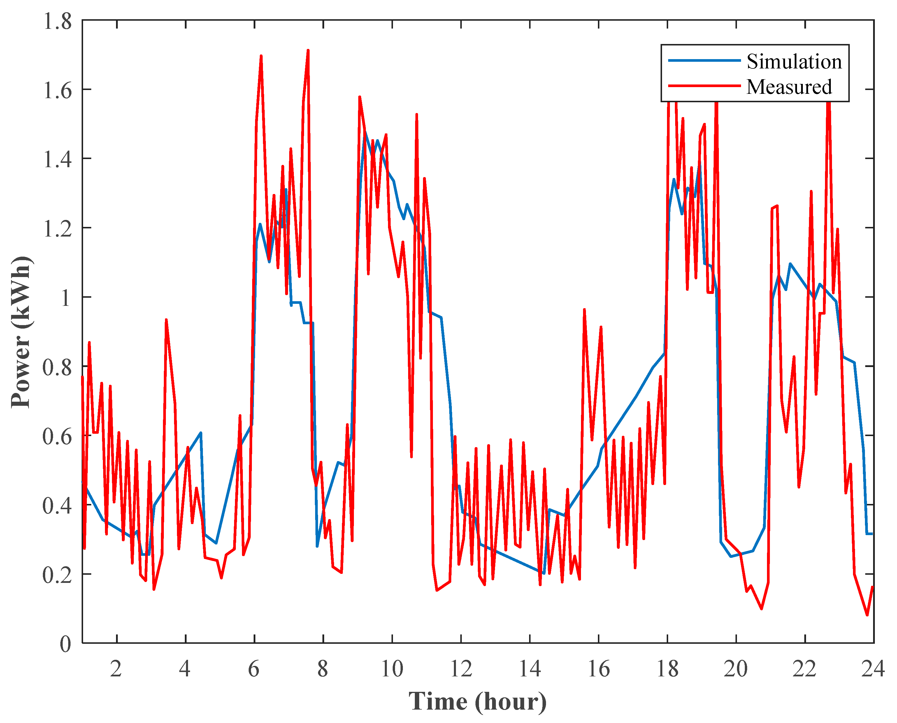
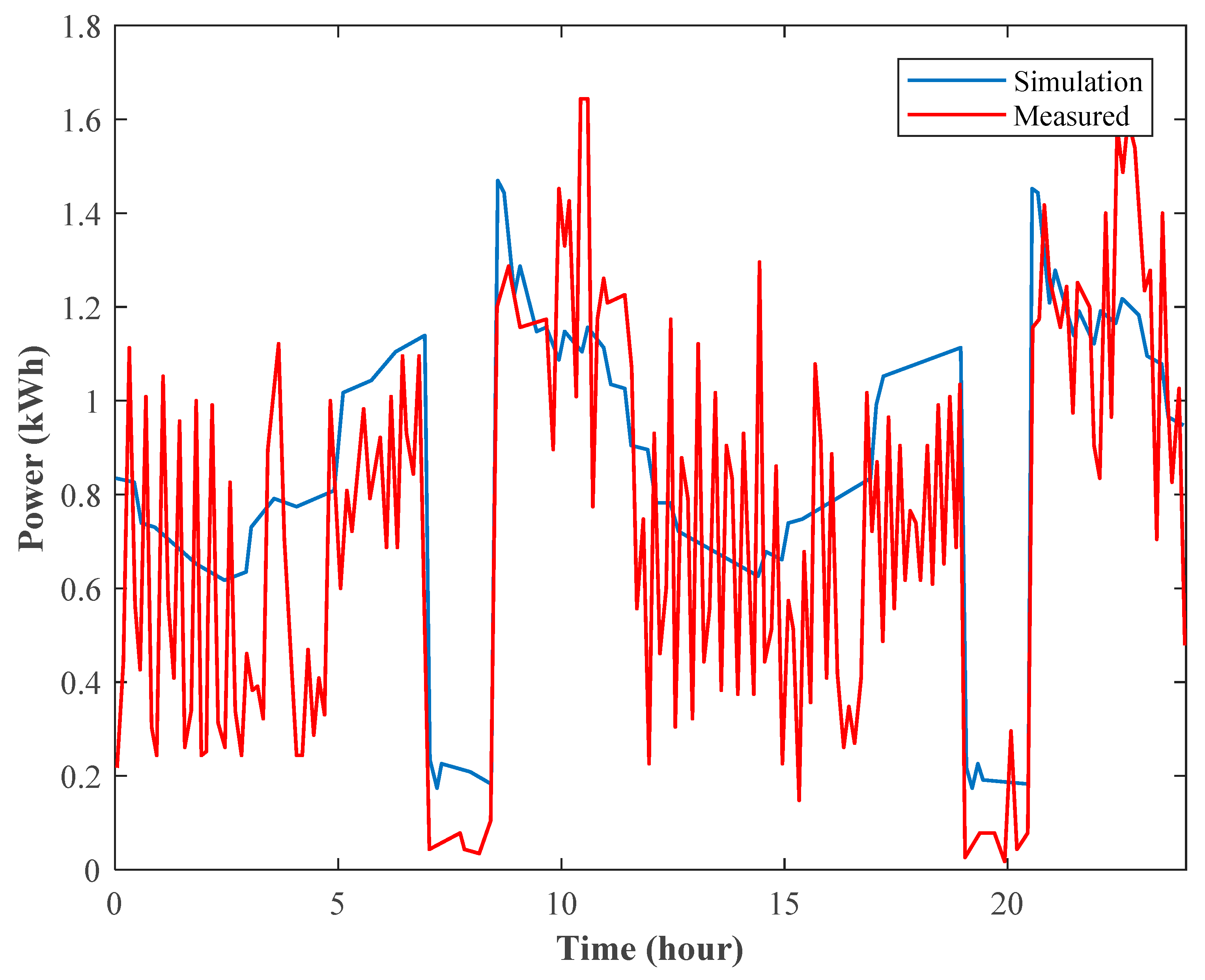
In addition to the statistical indicators, results from EnergyPlus simulation are directly compared to the empirical data, which was extracted from the electrical bills. Figure 2 compares the prediction of the electrical usage of different buildings by EnergyPlus and monthly electricity bills for these three sample buildings. As the Figure 3, Figure 4 and Figure 5 illustrate, simulation results followed the actual energy demands. Figure 3 and Figure 5 compare the results of simulation and measured data of three sample buildings. These graphs show that the hourly results also reasonably predict experimental data.

3.2. EnergyPlus Simulation Results

In this section, the crude results of the building energy simulation are presented. As previously mentioned, Energyplus based on the inputs, which consist of the geometry of a building, climate condition, and some other related parameters, can analyze the building, and calculate the energy usage of a building. Figure 6 shows the energy demand of building 2 for all hours in a year (this figure is based on the state B). As the figure shows, the energy required during the year has a large fluctuation, and it is maximum in summer months. Figure 7 depicts the energy production of the 2 kW PV system for the same building over a year. This graph shows more fluctuations at different times, because at some times there is no sunlight which can be used by the PV system to produce electricity. These two types of information for all buildings and price plans have been calculated in order to make the economic analysis possible.

3.3. Economical Comparison

Based on the building energy simulation results, a comparison between the annual electricity bills of the sample buildings with and without solar systems is presented in

Table 6. Annual payment for different scenarios.

PV Power (kW)	0	2	3	4	5	6	7
Annual Electricity costs Building 1-case 1 ($)	1579.28	1325.14	1258.42	1191.75	1128.41	1080.45	991.51
Annual Electricity costs Building 1-case 2 ($)	109272	940.25	883.39	834.47	789.21	745.87	703.62
Annual Electricity costs Building 2-case 1 ($)	1585.31	1277.44	1204.60	1131.94	1066.36	997.35	922.69
Annual Electricity costs Building 2-case 2 ($)	897.04	753.97	730.39	716.55	707.21	700.13	694.53
Annual Electricity costs Building 3-case 1 ($)	1229.03	1043.89	968.19	892.41	816.34	754.16	665.24
Annual Electricity costs Building 3-case 2 ($)	995.14	824.26	765.89	712.34	661.29	611.70	563.08

. These initial results indicate that by increasing the PV system’s size, the annual electricity bills decrease. However, Table 6 is not insightful enough, because it does not consider the price of the PV systems.

To fulfill the objectives of this study, a more detailed and in-depth analysis is required. It is necessary to determine what a PV system’s lifetime is. Most solar panel manufacturers offer a 10-year materials warranty, but the best solar panels come with a 12, 15, or even 25-year warranty. In this study, we, optimistically, consider the useful lifetime of the PV system to be 30 years. In addition, based on this lifetime, the results are subcategorized according to state surveyed.

3.4. State A

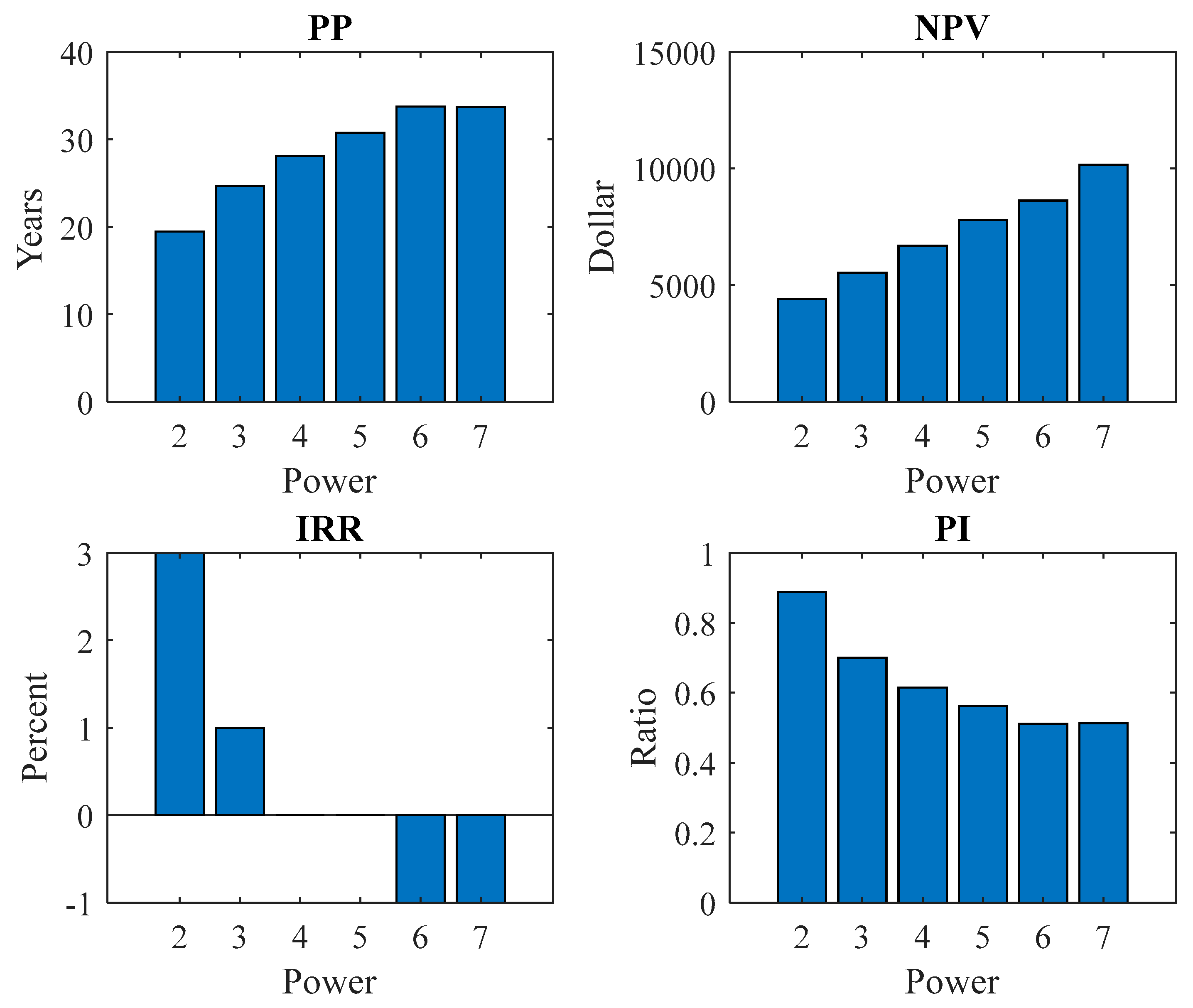
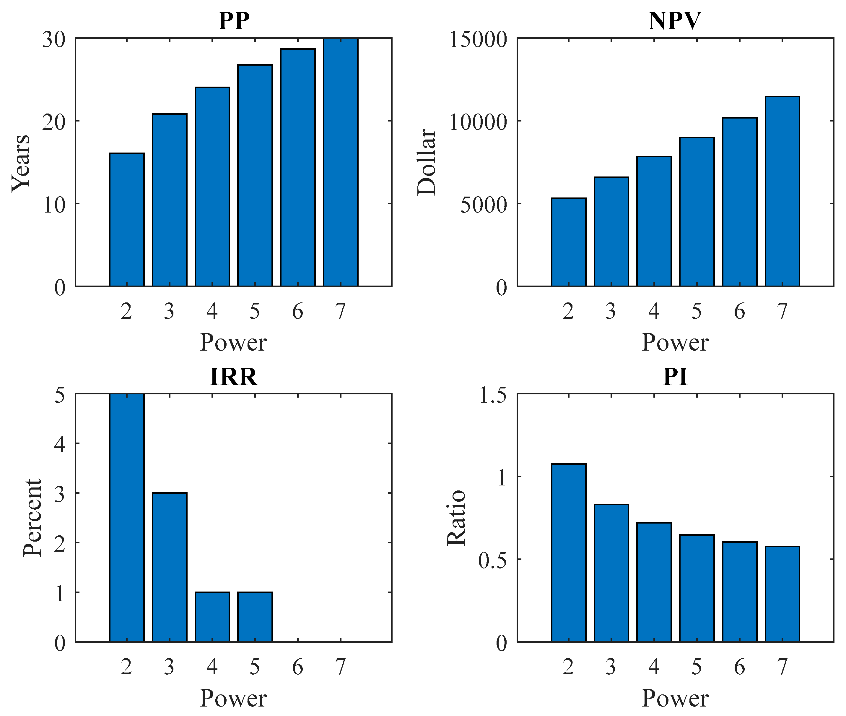
Figure 8, Figure 9 and Figure 10 show all the economic parameters explained above for buildings using different PV system sizes. In all cases, the parameters showed relatively similar behavior. PP for all the buildings and all the PV systems is more than 20 years (except for one, which is 19.5 years). These numbers are too large to be suitable for investment and therefore disappoint customers to invest in this sector.

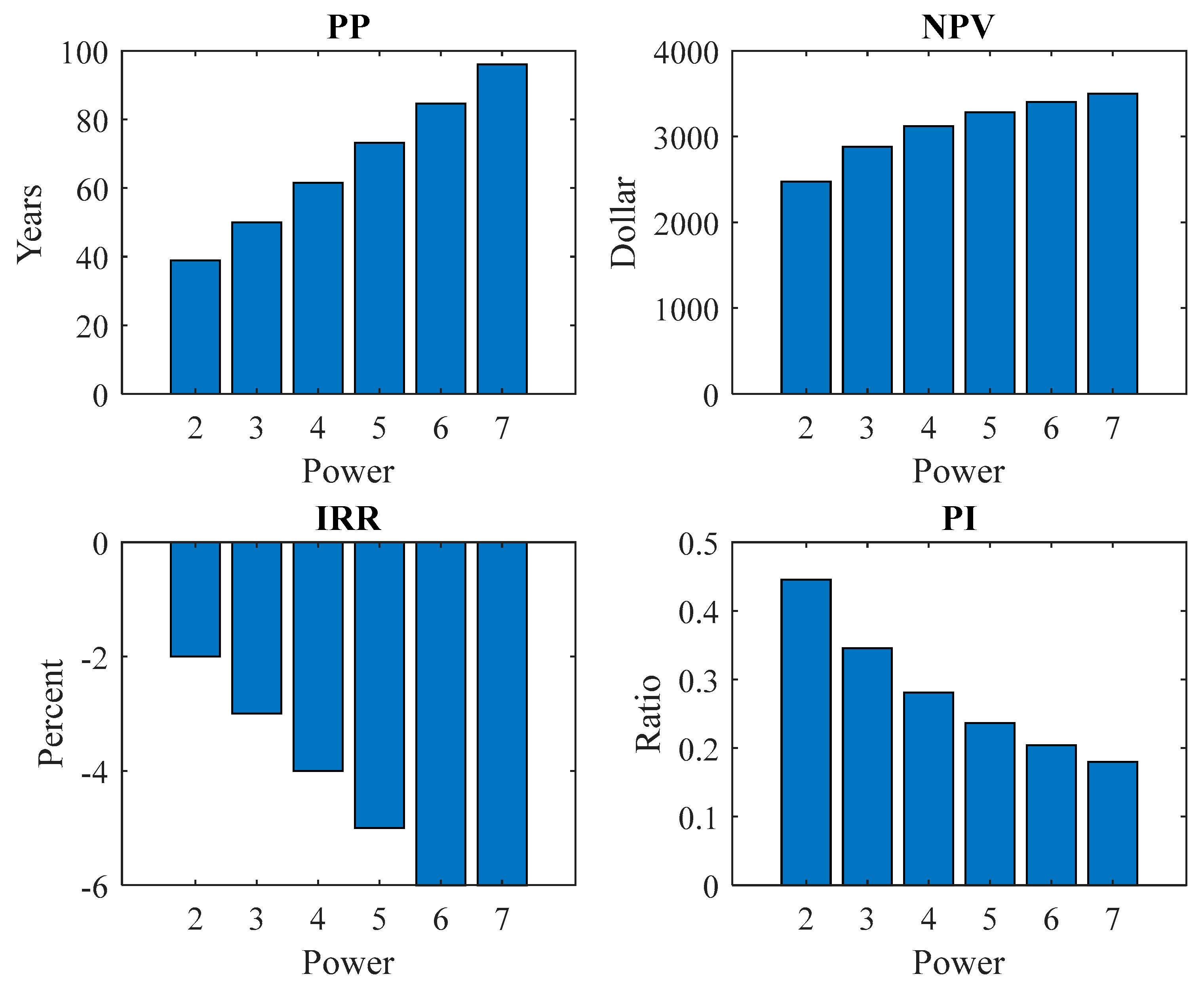
Another vital point to note is that PP is longer for bigger system sizes. In addition, NPV is plotted as a function of the PV system sizes (Figure 8). As shown in Figure 8, NPV decreases with increasing power systems due to higher initial costs. To understand better the value of investment, the NPV should be compared to the initial investment value, which is what PI does. As they are shown in Figure 8, Figure 9 and Figure 10, in all three cases and all power modes PI is less than one, which means investment, is not profitable. The way PI changes is similar to the PP, and it shows that the smaller systems represent higher profitability. IRR proves that almost, for every scenario of using the PV systems, investment is not desirable. IRR for every mode is equal to, or less than 4 percent and even for some cases is less than zero, which means acutely loss-making investment.

Figure 11 compares the economic parameters of the three buildings when they adopt solar systems for the state A. For this comparison, the smallest system size, which is the best scenario according to Figure 8, Figure 9 and Figure 10, is selected. Figure 11 shows that building 2, one-story concrete frame, has better results compared to the other two buildings. Building 2 has a lower PP and higher NPV, PI and IRR, which shows that all economic parameters indicate the superiority of investment in this type of building rather than others. Building 3, one-story wood frame, on the other hand, shows the worst results. By considering that the building 2 and 3 are both one-story homes, it can be argued that a concrete frame building is more capable of benefiting from solar energy in the presence of the demand charges rather than wood frame building in this state.

This analysis suggests that if the price plan described in Table 2 is applied, it is not a good idea to use the PV systems in state A. Although the federal government and state considered some sort of rebate for customers who use the PV systems, from a purely economic perspective, using a PV system is not reasonable.

3.5. State B

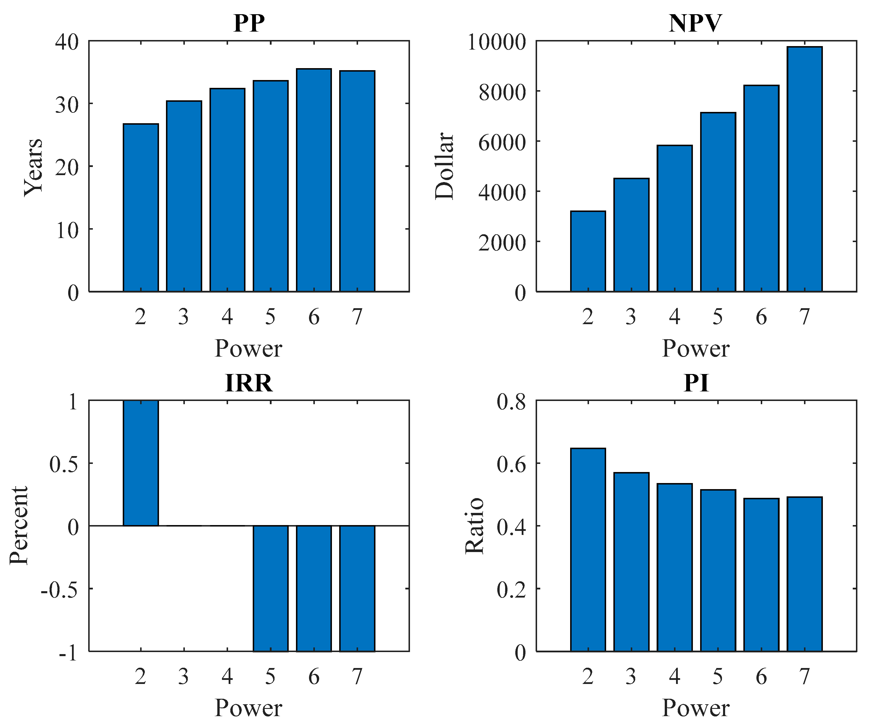
In this section, Table 3 is used to determine the impact of the price plans of case 2 on the use of the solar systems. Similar to the previous section, six different scenarios based on the PV power systems are considered. Figure 12, Figure 13 and Figure 14 evaluate these scenarios based on the price plans of state B. All of the PP values are in all cases more than 30 years, which means an investor must wait for at least 30 years to recover only its initial cost, which represents a detrimental investment. NPV or its improved version, PI supports this conclusion. All of the PI values are less than one, which shows the investment is not profitable. IRR like other parameters shows the loss-making of this investment. Moreover, IRR analysis shows that larger system sizes are less suitable when demand charges are applied.

Figure 15 compares the economic parameters studied for the three building types when a 2 kW solar system is installed. Precisely opposite to state A, building 3, with a one-story wood frame, is the best choice for using the PV systems and building 2, a one-story concrete block, has the worst performance.

Figure 16 compares the results of the two states considering the building type 1 with a 2 kW solar system. The economic parameters are normalized based on the absolute maximum of each parameter. This figure shows that using the PV system in state A has a better economic justification than state B.

4. Conclusions

This study examines the performance of the PV systems in the residential buildings in the presence of the demand charges. For a comprehensive review, two distinct regions (state A and B) and three different building types are investigated. This paper aimed to show the total cost savings (if any), to evaluate the economic parameters of investment in this area for a customer. To avoid repetition, the environmental impacts of the PV systems are not considered, and from a purely economic perspective, the profitability of these systems in the presence of the demand charges is investigated.

In state A, the results show that due to the demand charge tariffs, using the PV system has no economic justification. All of the financial parameters unanimously show that investing in a PV system is loss-making. Another point is that the smaller the purchased system, the less loss-making consequences will be observed. There is almost a linear relationship between increasing the size of the purchased system and the resulting loss. In state A, the best candidate for installing the PV system is a one-story concrete frame, and the worse one is a one-story wood frame. It should be noted that these results are highly sensitive to the price of tariffs.

Results were almost the same for state B. It can be concluded that the payback period is too extended to be desirable, the rate of return is too low, and the value of the profitability index for investment is low. As these parameters show, using solar system in the state B is also loss-making. As the solar system size increases, the economic parameters declare that the investment is more unsatisfactory. In state B, exactly opposite to state A, the one-story concrete frame shows the worst result, and the one-story wood frame was the best candidate for the investment. The comparison between different buildings depends more on the material used on them, rather than the price plan. Therefore, no claim can be made about the suitability of one of the buildings than the rest in using solar energy. These results prove that the price plan has a decisive role in loss-making or profitability of using the PV systems. The last point from which can be concluded is that, by this tariff, state A is better for using the PV system rather than state B, even as it is not desirable.

There is no doubt that the solar energy, particularly the PV system is very environmentally friendly, but despite the many advances made in using and constructing them and their sharp price drop sover the past decades, they are still not profitable in the presence of the demand charges. This paper, in a very optimistic way, ignores the maintenance and other costs of the PV system, but even in this scenario, using the PV system with the presence of the demand charge has no justification.

References

- Horrigan, L.; Robert, S.L.; Walker, P. How sustainable agriculture can address the environmental and human health harms of industrial agriculture. Environ. Health Perspect. 2002, 110, 445–456. [Google Scholar] [CrossRef] [PubMed]
- Chu, S.; Cui, Y.; Liu, N. The path towards sustainable energy. Nat. Mater. 2017, 16, 16. [Google Scholar] [CrossRef] [PubMed]
- Solomon, S.; Qin, D.; Manning, M.; Averyt, K.; Marquis, M. Climate Change 2007—The Physical Science Basis: Working Group I Contribution to the Fourth Assessment Report of the IPCC; Cambridge University Press: Cambridge, UK, 2007; Volume 4. [Google Scholar]
- Berinstein, P. Alternative Energy: Facts, Statistics, and Issues; Oryx Press: Westport, CT, USA, 2001; pp. 1–190. [Google Scholar]
- Foster, R.; Ghassemi, M.; Cota, A. Solar Energy: Renewable Energy and the Environment; CRC Press, Taylor & Francis Group: Boca Raton, FL, USA, 2010; pp. 233–248. [Google Scholar]
- Masschelein, W.J.; Rice, R.G. Ultraviolet Light in Water and Wastewater Sanitation; CRC Press: Boca Raton, FL, USA, 2016. [Google Scholar]
- Renewable Energy Policy Network for the 21st Centry. Global Status Report; REN21 Secretariat: Paris, France, 2016. [Google Scholar]
- Breyer, C.; Bogdanov, D.; Gulagi, A.; Aghahosseini, A.; Barbosa, L.S.; Koskinen, O.; Barasa, M.; Caldera, U.; Afanasyeva, S.; Child, M. On the role of solar photovoltaics in global energy transition scenarios. Progr. Photovolt. Res. Appl. 2017, 25, 727–745. [Google Scholar] [CrossRef]
- Solangi, K.; Islam, M.; Saidur, R.; Rahim, N.; Fayaz, H. A review on global solar energy policy. Renew. Sustain. Energy Rev. 2011, 15, 2149–2163. [Google Scholar] [CrossRef]
- Brito, M.; Gomes, N.; Santos, T.; Tenedório, J. Photovoltaic potential in a lisbon suburb using lidar data. Sol. Energy 2012, 86, 283288. [Google Scholar] [CrossRef]
- Grätzel, M. Photoelectrochemical cells. Nature 2001, 414, 338. [Google Scholar] [CrossRef] [PubMed]
- Grubišić-Čabo, F.; Nižetić, S.; Giuseppe Marco, T.J.T.O.F. Photovoltaic panels: A review of the cooling techniques. Trans. FAMENA 2016, 40, 63–74. [Google Scholar]
- Das, N.; Wongsodihardjo, H.; Islam, S.J.R.E. Modeling of multi-junction photovoltaic cell using matlab/simulink to improve the conversion efficiency. Renew. Energy 2015, 74, 917–924. [Google Scholar] [CrossRef]
- Das, N.; Wongsodihardjo, H.; Islam, S. A preliminary study on conversion efficiency improvement of a multi-junction pv cell with mppt. In Smart Power Systems and Renewable Energy System Integration; Springer: Berlin, Germany, 2016; pp. 49–73. [Google Scholar]
- Hammonds, M. Getting power from the sun. Chem. Ind. 1998, 6, 219. [Google Scholar]
- Burns, J.E.; Kang, J.-S. Comparative economic analysis of supporting policies for residential solar pv in the united states: Solar renewable energy credit (srec) potential. Energy Policy 2012, 44, 217–225. [Google Scholar] [CrossRef]
- Nejat, P.; Jomehzadeh, F.; Taheri, M.M.; Gohari, M.; Majid, M.Z.A. A global review of energy consumption, CO2 emissions and policy in the residential sector (with an overview of the top ten CO2 emitting countries). Renew. Sustain. Energy Rev. 2015, 43, 843–862. [Google Scholar] [CrossRef]
- Nižetić, S.; Papadopoulos, A.; Tina, G.; Rosa-Clot, M.J.E. Hybrid energy scenarios for residential applications based on the heat pump split air-conditioning units for operation in the mediterranean climate conditions. Energy Build. 2017, 140, 110–120. [Google Scholar] [CrossRef]
- Bernal-Agustín, J.L.; Dufo-López, R. Economical and environmental analysis of grid connected photovoltaic systems in spain. Renew. Energy 2006, 31, 1107–1128. [Google Scholar] [CrossRef]
- Oliver, M.; Jackson, T. Energy and economic evaluation of building-integrated photovoltaics. Energy 2001, 26, 431–439. [Google Scholar] [CrossRef]
- Shaw-Williams, D.; Susilawati, C.; Walker, G. Value of residential investment in photovoltaics and batteries in networks: A techno-economic analysis. Energies 2018, 11, 1022. [Google Scholar] [CrossRef]
- Mahmud, M.; Huda, N.; Farjana, S.; Lang, C. Environmental impacts of solar-photovoltaic and solar-thermal systems with life-cycle assessment. Energies 2018, 11, 2346. [Google Scholar] [CrossRef]
- Shah, S.; Valasai, G.; Memon, A.; Laghari, A.; Jalbani, N.; Strait, J. Techno-economic analysis of solar pv electricity supply to rural areas of Balochistan, Pakistan. Energies 2018, 11, 1777. [Google Scholar] [CrossRef]
- Zsiborács, H.; Baranyai, N.H.; Vincze, A.; Háber, I.; Pintér, G. Economic and technical aspects of flexible storage photovoltaic systems in Europe. Energies 2018, 11, 1445. [Google Scholar] [CrossRef]
- Kolhe, M.; Kolhe, S.; Joshi, J. Economic viability of stand-alone solar photovoltaic system in comparison with diesel-powered system for India. Energy Econ. 2002, 24, 155–165. [Google Scholar] [CrossRef]
- Ajan, C.W.; Ahmed, S.S.; Ahmad, H.B.; Taha, F.; Zin, A.A.B.M. On the policy of photovoltaic and diesel generation mix for an off-grid site: East malaysian perspectives. Sol. Energy 2003, 74, 453–467. [Google Scholar] [CrossRef]
- Nafeh, E.-S.A. Design and economic analysis of a stand-alone PV system to electrify a remote area household in Egypt. Open Renew. Energy J. 2009, 2, 33–37. [Google Scholar] [CrossRef]
- Ojosu, J. The iso-radiation map for Nigeria. Sol. Wind Technol. 1990, 7, 563–575. [Google Scholar] [CrossRef]
- Rodrigues, S.; Chen, X.; Morgado-Dias, F.J.E.P. Economic analysis of photovoltaic systems for the residential market under China’s new regulation. Energy Policy 2017, 101, 467–472. [Google Scholar] [CrossRef]
- Rodrigues, S.; Faria, F.; Cafôfo, N.; Chen, X.; Mata-Lima, H.; Morgado-Dias, F.J.J.C.E.T. Analysis of the self-consumption regulation for photovoltaic systems with battery banks in the portuguese residential sector. J. Clean. Energy Technol. 2017, 5, 52–59. [Google Scholar] [CrossRef]
- Rodrigues, S.; Torabikalaki, R.; Faria, F.; Cafôfo, N.; Chen, X.; Ivaki, A.R.; Mata-Lima, H.; Morgado-Dias, F.J.S.E. Economic feasibility analysis of small scale PV systems in different countries. Sol. Energy 2016, 131, 81–95. [Google Scholar] [CrossRef]
- Arababadi, R.; Parrish, K. Modeling and testing multiple precooling strategies in three residential building types in the phoenix climate. ASHRAE Trans. 2016, 122, 202–214. [Google Scholar]
- Arababadi, R.; Parrish, K. Reducing the need for electrical storage by coupling solar pvs and precooling in three residential building types in the phoenix climate. ASHRAE Trans. 2017, 123, 279–290. [Google Scholar]
- Griffith, B.T.; Ellis, P. Photovoltaic and Solar Thermal Modeling with the Energyplus Calculation Engine; National Renewable Energy Lab.: Golden, CO, USA, 2004. [Google Scholar]
Figure 1.
Selected sample buildings: (a) two-story wood frame (Building 1), (b) one-story concrete block (Building 2), and (c) one-story wood frame (Building 3).
Figure 2.
Comparison between simulated and monthly bill electricity usage of different buildings.
Figure 3.
Simulated and measured hourly electricity usage of building 1.
Figure 4.
Simulated and measured hourly electricity usage of building 2.
Figure 5.
Simulated and measured hourly electricity usage of building 3.
Figure 6.
Energy demand for building 1.
Figure 7.
Energy production of 2 kW PV system for building 1.
Figure 8.
Economic parameters of building 1 in the state A.
Figure 9.
Economic parameters of building 2 in the state A.
Figure 10.
Economic parameters of building 3 in the state A.
Figure 11.
Comparing different buildings in the state A.
Figure 12.
Economic parameters of building 1 in the state B.
Figure 13.
Economic parameters of building 2 in the state B.
Figure 14.
Economic parameters of building 3 in the state B.
Figure 15.
Comparing different buildings in the state B.
Figure 16.
Compare the economic justification of two states. (1) State A (2) State B.