Impact Evaluation of Wind Power Geographic Dispersion on Future Operating Reserve Needs

Abstract

This paper evaluates the potential of diverse wind power patterns to balance the global power output of wind farms using the concept of operating reserve assessment. To achieve this, operating reserve assessment models are utilized to evaluate bulk generation systems under several conditions of wind power geographic distribution. Different wind behavior patterns and wind power penetration levels are tested using a modified configuration of the Institute of Electrical and Electronics Engineers Reliability Test System 96 (IEEE RTS-96). The results highlight that on a large country scale system with different wind characteristics, the diversification of wind behavior might be conducive to a compensation of wind power fluctuations, which may significantly decrease the need for system operating reserves. This effect is verified using probability distribution functions of reserve needs estimated by sequential Monte Carlo simulations (SMCS), such that useful information regarding generation capacity flexibility is drawn from the evaluations.

1. Introduction

Wind farm reliability is a subject of interest to industry and academia [1,2,3,4]. The availability of wind as a resource alongside the reliability of wind turbine generators may significantly affect power system reliability [5,6,7,8,9,10,11,12]. As a general concept, wind power diversification means that different wind farms can complement each other, leading to a smoother global power output [13,14,15,16]. There is clearly an understanding that the geographic dispersion of wind power outputs, through the combination of negative and positive correlations, might reduce the variability of the total power produced by wind turbines [17].

Due to the growing diffusion of wind energy into the energy matrix of current power systems, the design of future generating systems using only static reserve assessments does not seem to be enough to ensure the security of the power system operation. Usually, operating reserve is a concern of short-term operating planning [18,19], and few works in the technical literature have explored the concept of operating reserve for medium- and long-term analysis [20,21]. Hence, it is of interest to measure the impact of geographic dispersion on future operating reserve needs, bearing the system performance in mind. Clearly, one of the disadvantages of this approach is the number of uncertainties to be addressed into the medium- and long-term operating planning. For instance, for planners, it is impossible to assure that a specific generating unit will be available to be dispatched in a given time instant of the future. However, it is plausible to assume that part of the current generating units will be available to be dispatched, considering current and new generating units and a considerable number of wind turbines. On the other hand, one of the main advantages of the approach is providing system planners with reliable information about the use of high levels of wind power, and assuring that investment options will result in more robust and flexible generating configurations in accordance to the wind potential of different areas.

The combination of various wind power patterns introduced by a significant penetration of geographically dispersed wind farms naturally introduce some patterns of interest to the system operation. Conversely, for system adequacy evaluations, inside the same site it can be assumed that turbine outputs present similar patterns, mainly due to the same wind characteristic. In order to make a prognosis of the generation performance at multiple wind farms, a wind measurement campaign is typically conducted for 1–3 years at several locations across the site [22]. Ideally, such a campaign should be able to estimate geographical variability in the wind power generation to investigate to what extent such variability may be smoothed through national interconnections. A combination of results from such campaigns with risk-based methodologies to evaluate system operational responses for the long-term can be performed, mainly using long-term operational reserve methodologies [10,20,21]. Such evaluation is essentially dependent on the quality of the campaign results. Usually, in the medium- and long-term, it is not possible to know precisely the availability of generating units and their conversion technologies at each operation moment as in traditional short-term operating reserve evaluation [18,19]. Therefore, the risk analysis must be focused towards system performance evaluations [7,10,20,21], aiming at decisions that will result in a more reliable generation system. From a technological perspective, the design characteristics of conventional hydro and thermal generators already enable the generating units to contribute to system support services, such as voltage and frequency regulation [23]. Conversely, wind generators are not capable of fully providing the same system support services as large hydro or thermal generating units. Moreover, from an integration perspective, wind generation imposes additional requirements, mainly due to the inherent unpredictable and volatile characteristics of the wind. Also, more flexible conventional generators (hydro and thermal-gas) might be required to provide adequate system support services.

Within this context, this paper evaluates the benefits of wind power geographic dispersion on reserve needs using operating reserve assessment models. Different wind behavior patterns and wind power penetration levels are tested using a modified configuration of the IEEE RTS-96. The effect of wind power geographic dispersion is verified using probability distribution functions of reserve needs estimated using a sequential Monte Carlo approach, such that useful information regarding generation capacity flexibility is drawn from the evaluations.

The paper is organized as follows. Section 2 introduces the approach utilized to evaluate the impact of geographic dispersion of wind power. Section 3 discusses the benefits of wind power geographic dispersion on reserve needs. Section 4 shows the results of the applied evaluation for a test system, and Section 5 presents conclusions and final remarks.

2. Evaluation Approach

Diversification can be used to reduce the overall variation of the power output of various wind farms. Degeilh and Singh [13] proposed an optimization technique to distribute a given number of wind turbines over a given number of sites so as to minimize the variance while keeping the mean power output essentially unchanged. This process can be used as an aid in site selection. These references also show that reducing the variance tends to reduce the loss of load expectation.

The difficulty is that the number of random variables involved in this problem is so large that it is necessary to make some assumptions and often the sites may be selected depending on the geographical and ecological considerations. Following a different approach, we examine diversification from the operating reserve perspective, aiming to evaluate the benefit of geographically dispersed wind farms through uncertainty models. The uncertainty related to the operating reserve is caused by the intermittency of the primary energy resources ($∆W_S$), the forced outages of the generating units ($∆G$) and the randomness of the system load ($∆L$). Therefore, it is possible to model operational procedures to assess the adequacy of the operating reserve using a planning perspective, which in fact can be named as operating reserve capacity (ORC) evaluation.

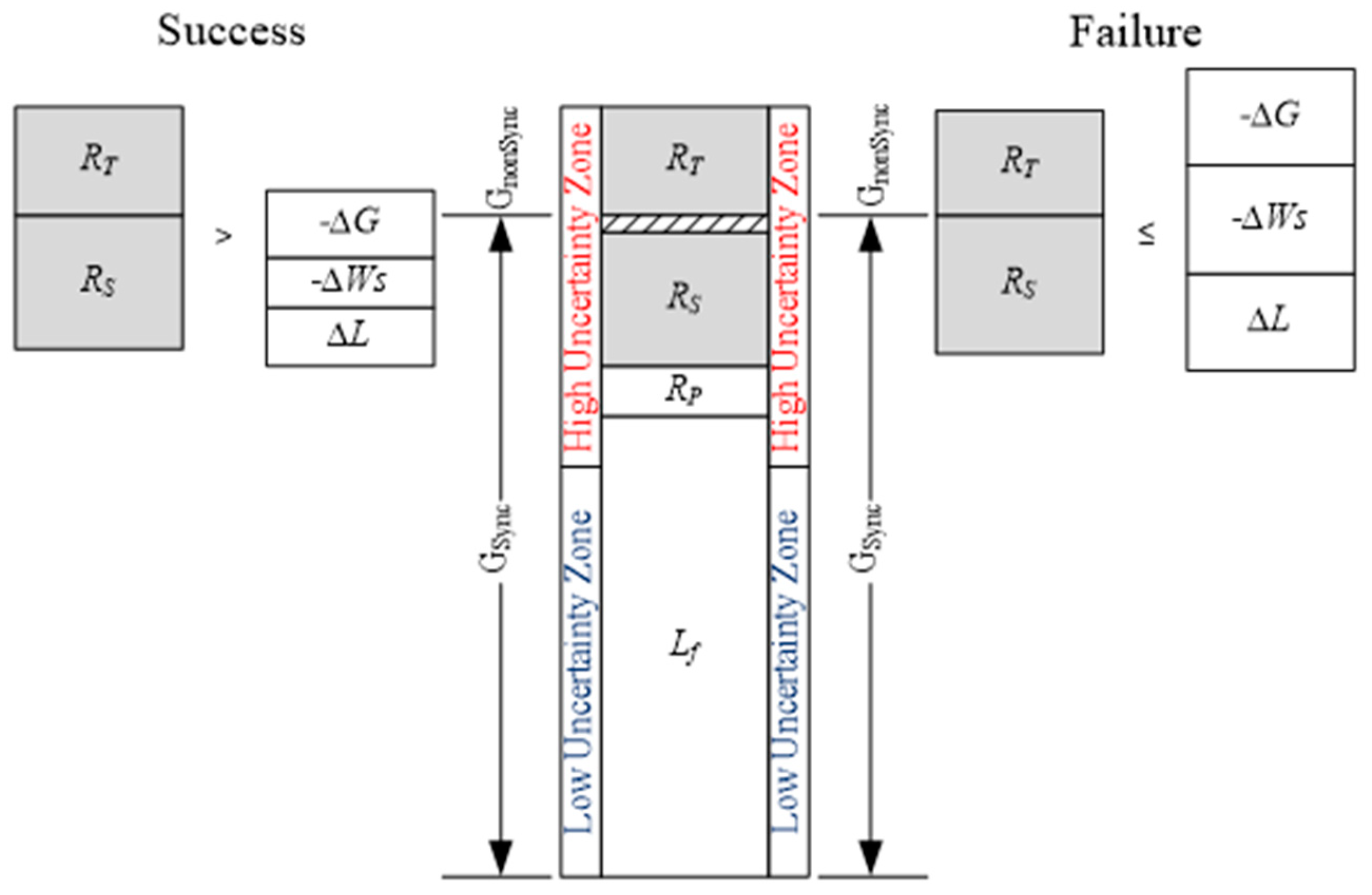
The ORC consists of the secondary reserve plus the fast tertiary reserve available at the moment of the evaluation. The fast tertiary means generating capacity that is not committed. However, these are special units capable of taking load in a short period of time, such as 1 h. Applying a simple scheduling procedure, the identification of the events of insufficient operating reserve capacity is made according to Equation (1) as

$$R_S+R_T-\left(∆L-∆W_S-∆G\right)\le 0.$$

(1)

in which R_S is the secondary reserve requirement, R_T is the fast tertiary reserve, and $∆$L and $∆$W_S are the system load and system wind power forecast errors at the moment of the evaluation, respectively. The variable $∆G\left(t\right)$ is given by the generation units that have been committed but are out of service at instant t, i.e., it consists of non-committed generation capacity which would meet the following: The system load forecasted $L_f\left(t\right)$ at instant t, the primary reserve $R_P$ and secondary reserve $R_S$ requirements. Equation (2) presents this condition,

$$∆G\left(t\right)=G_{SYNC}\left(t\right)-\left(L_f\left(t\right)+R_P+R_S\right).$$

(2)

where $G_{SYNC}\left(t\right)$ is the total generation capacity synchronized at instant t.

This novel perspective may be summarized in Figure 1, and can be viewed as a way to assess, in terms of flexible capacity, the future generation system to accommodate a large percentage of wind power. As shown in Figure 1, the success and failure states are properly verified if the operating reserve capacity is sufficient or not to compensate for the difference between load and generation deviations at each hour t, during an established observation time.

The SMCS makes it possible to keep track of several features related to the operating history of system states. Its flexibility also makes it possible to model details about uncertainties, which are not addressed in traditional (deterministic) methods. In the simulation, the time duration of each generating unit in given state (failure or operating) is sampled according to a probability distribution, such as the exponential distribution.

$$T_{up}=-\frac{1}{\lambda }\ln U$$

(3)

$$T_{dw}=-\frac{1}{\mu }\ln U$$

(4)

where $T_{up}/T_{dw}$ is the time duration in the operating/failure state, $\lambda$ is the failure rate of the unit, $\mu$ is the repair rate of the unit and $U$ is a uniformly distributed random number sampled in [0, 1].

The loading and wind at a given time instant is simulated using sampled curves. Whereas a state transition is assigned, the set of states is evaluated using Equation (1). After evaluating each system state, performance indices are estimated using the expected value equation [24]:

$$E\left[\mathit{H}\right]=\frac{1}{N}{\displaystyle \sum }_{u=1}^{N}H\left(y_u\right)$$

(5)

where y_u is the sequence of system states in year u, H(y_u) is the reliability test function evaluated at y_u, N represents the number of simulated years (samples), and H is the random variable which maps H(y_u) values. The uncertainty surrounding the estimated indices is given by the variance of the estimative [24]

$$V\left[E\left[\mathit{H}\right]\right]=\frac{V\left[\mathit{H}\right]}{N}$$

(6)

and the stochastic process convergence is tested using the coefficient of variation β [24].

$$\beta =\frac{\sqrt{V\left[E\left[\mathit{H}\right]\right]}}{E\left[\mathit{H}\right]}$$

(7)

Following these definitions, the conventional system reliability indices may be estimated. This traditional view can provide important information on loss of load events and, in this case, it will monitor the successes and failures of the static and operating reserves, where the following reliability indices will be used [21]: Loss of Load Probability (LOLP), Loss of Load Expectation (LOLE, in h/y, Expected Energy Not Supplied (EENS, in MWh/y), Loss of Load Frequency (LOLF, in occ./y), and Loss of Load Duration (LOLD, in h/occ.). In this paper, another set of random variables will be monitored. By using the same concepts presented in Equations (5)–(7), the uncertainties surrounding the operating reserve concept will be monitored to investigate, in detail, the probability distribution functions linked to the performance of the operating reserve from a long-term perspective. The following sections will introduce all of these deviations as random variables.

In this planning context, it is essential to enforce not only system capacity, but also system flexibility, in order to prepare the future generation system to handle the entire set of uncertainties.

3. Impact of Wind Power Geographic Dispersion on Reserve Needs

3.1. Upscaling Model of Dispersed Wind Power

In order to verify the impact of wind power geographic dispersion on operation reserve capacity, the upscaling behavioral model of dispersed wind power must be obtained through real data. The generation systems with predominant coal-fired power plants have reduced system operational flexibility to accommodate large-scale wind power integration [25]. The hydro units using reservoirs offer a capability to start in a short time and thus provide more flexibility. Notwithstanding, one of the most popular hydro generation systems in the world is the run-of-river that also offers reduced system operational flexibility [26]. This simplest form of generation includes not only simple construction aspects, but also the aggregation of other functions linked to environmental concerns, such as flood control and agricultural irrigation. When combining both thermal and wind power sources, the result is an energy portfolio with reduced generation flexibility characteristics. After analyzing several different types of wind behavior, wind farms located in the Rocky Mountains region (USA) were chosen to perform this evaluation [27]. The choice was based on the wind diversity in this geographic area, where each wind farm has a different behavior, although they are in the same region. However, the area is large enough to justify this situation and the six wind farms can properly characterize good wind diversity. For instance, from the ordinary statistical measurements, it is possible to identify that the Rocky Mountains time-series for the year 2004 presents very regular measurements. As a matter of fact, wind farms 6673, 21777 and 23353 have an average production (p.u.) and standard deviation (p.u.) of (0.31; 0.34), (0.32; 0.34) and (0.35; 0.34), respectively. On the other hand, the wind farms 20144, 29617 and 29863 have an average production (p.u.) and standard deviation (p.u.) of (0.26; 0.31), (0.20; 0.28) and (0.20; 0.28), respectively.

From the variability point of view, the number of upward and downward wind ramp occurrences is of major relevance. Using a simple ramp concept where a ramp event is considered to occur at the start of an interval if the magnitude of the increase or decrease in generation at a time period ahead of the interval is greater than the pre-defined threshold [28].

Table 1. Number of upward ramps in 1 h: Rocky Mountains series.

PU	6673	20144	21777	23353	29617	29863	Sum
0.1	1326	923	1081	996	643	604	284
0.2	625	385	431	336	240	187	29
0.3	314	185	200	117	86	67	3
0.4	162	78	83	47	36	23	1
0.5	59	35	36	19	15	13	0
0.6	22	15	16	6	9	5	0
0.7	4	3	5	2	3	2	0
0.8	2	1	0	0	0	0	0
0.9	2	1	0	0	0	0	0
1.0	0	0	0	0	0	0	0

and

Table 2. Number of downward ramps in 1 h: Rocky Mountains series.

PU	6673	20144	21777	23353	29617	29863	Sum
0.1	1276	949	1081	962	654	611	274
0.2	631	336	418	296	185	167	16
0.3	322	130	158	117	66	55	2
0.4	170	52	71	46	24	27	0
0.5	86	21	29	10	13	12	0
0.6	44	11	13	5	5	4	0
0.7	11	3	2	3	3	2	0
0.8	3	2	1	0	0	0	0
0.9	0	2	0	0	0	0	0
1.0	0	0	0	0	0	0	0

provide the number of ramp occurrences between 0.10 and 1.00 p.u. of generation within 1 h for the wind farms quoted previously. The observations are in both upward and downward directions. This measurement of variability in these time-series may represent a simple view on flexibility requirements [29] within 1 hour of the generation systems due to wind power integration. Data analysis can show that the time-series with 0.31 p.u. of average generation presents a considerable number of ramp occurrences when compared to the time-series with 0.20 p.u. of average generation. The number of ramp occurrences above or equal to 0.40 p.u. is significant in both cases when the time-series is annual. In this case, the number of ramp occurrences above or equal to 0.70 p.u. is lower in the upward direction than in the downward direction. However, the total number of occurrences is higher in the upward direction than in the downward direction. Also, the compensation effect can be verified in the last column, corresponding to a synthetic series composed of the sum of the Rocky Mountains series. Several other analyses may be possible when comparing these wind farms. Nevertheless, a major characteristic shown in Table 1 and Table 2 is that the variability presented in all wind farms may require operational system flexibility. However, it is extremely important to investigate aspects related to the correlation of wind generation, where such amounts of wind power variations may be moderated by a smoothing effect caused by geographic dispersion [17]. The next subsection will outline the impact of system uncertainties on ORC.

3.2. System Uncertainties Impact on Operating Reserve

The aforementioned system uncertainties may be viewed as exerting a positive or negative impact on the system balance, depending on how suddenly they occur and the magnitude and direction of their variations. The SMCS method is the one that better represents the chronological and uncertainty aspects, such as the wind power annual series, related to the wind behavior. Hence, the SMCS algorithm introduced in References [20,21] was enhanced to include the wind dispersion behaviors sampled according to their region. By modeling $∆L$, $∆W_S$ and $∆G$ as independent random variables [30], the aim is to evaluate the required and unrequired reserve, as well as their probability distribution functions, due to the geographic dispersion of wind power generators. Behind these models there is the complex relationship between these variables, which results in high levels of uncertainties for the unit commitment procedure.

Table 3. System uncertainties impact on operating reserve.

Classification	Variables			Conditional	Dev.	Reserve Consequence
ID.	ΔLf	ΔG	ΔWs	If	D	Up or Down
A	+	−	−		−	UPWARD
B	−	−	−	(ΔG + ΔWs) ≥ ΔLf	+	DOWNWARD
	−	−	−	(ΔG + ΔWs) < ΔLf	−	UPWARD
C	+	0	−		−	UPWARD
D	−	−	+	ΔG ≥ (ΔLf −ΔWs)	+	DOWNWARD
	−	−	+	ΔG < (ΔLf −ΔWs)	−	UPWARD
E	+	−	+	(ΔG − ΔLf) ≥ −ΔWs	+	DOWNWARD
	+	−	+	(ΔG − ΔLf) < −ΔWs	−	UPWARD
F	+	0	+	ΔWs ≥ ΔLf	+	DOWNWARD
	+	0	+	ΔWs < ΔLf	−	UPWARD
G	−	0	−	ΔWs ≥ ΔLf	+	DOWNWARD
	−	0	−	ΔWs < ΔLf	−	UPWARD
H	−	0	+		+	DOWNWARD

shows a summary of consequences (upward or downward reserve) that should be monitored during the adequacy evaluation of the generating system.

The power balances captured during the simulation may have negative or positive system effects with upwards or downwards reserve as a consequence. Table 3 highlights a collective perception between these variables concerning the operating perspective, where it will be possible to identify the negative correlation impact of different wind power outputs on the reliability indices. Another point of view will explore an individual perception of these variables through the investigation of the distributional aspects associated with each uncertainty representation. Table 3 decouples two categories of events: The deviation events A, B, D and E, which involve load deviations, wind power deviations, and generating outage deviations; and the deviation events C, F, G, and H, which only involve load and wind power deviations.

4. Results and Discussion

One of the main concerns of a system planner is to size generation equipment, mainly for meeting the load growth and to achieve certain spinning reserve requirements. In general, generation systems must be sized with sufficient capacity, flexibility and robustness to respond to several operational challenges. However, the volatility and variability that comes from renewable generation is a relatively recent concern for the system planners [26]. Hence, the evaluation of operating reserve capacity presented in this section will focus on conventional reliability evaluation, highlighting traditional reliability indices from two different aspects, i.e., static and operating reserve capacities. The evaluation exploits the probability distribution functions of reserve needs and unneeded reserve to verify the impact of geographic dispersion on reserve requirements.

Firstly, the proposed evaluation will follow the modified configuration of IEEE RTS-96 HW [21]. To cope with the power fluctuations of the hydro units, a set of five historical hydro series, referring to the average monthly power capacity used in Reference [21] and will stay without changes in this paper. Nevertheless, to cope with the power fluctuations of the wind power, some changes in Reference [21] are proposed. Initially, the same amount of wind power will be used, where a 350 MW of coal-fired unit is replaced by 1526 MW of wind power. Therefore, the original installed capacity of 10,215 MW will increase to 11,391 MW and the percentage of renewable power goes to 21.3%, considering hydro and wind production. The thermal generation subsystem consists of 77 units varying from 12 up to 400 MW and the hydro subsystem remains with 18 units of 50 MW each.

The proposed change is carried out on the wind subsystem, where the 763 wind turbines with 2 MW each remain the same, maintaining their distributed characteristics spread over three different regions or areas. In Reference [21] it is assumed that the wind behavior is a characteristic that is linked to the region or area. In this paper, it will be assumed that the wind behavior is a characteristic of the wind farm (a group of wind turbine very near), where each wind farm has its own wind behavior. Clearly, inside a region or area it is possible to install several wind farms. Similar to the Rocky Mountains region previously assessed in Section 3, this paper will assign a different wind behavior to each wind farm with a diversified wind characteristic. In this proposed evaluation, 763 wind turbines are distributed over 20 wind farms in three different regions. This contains a historical wind time-series, on an hourly basis, of the 3 different years equally probable and referring to the average power produced by a wind turbine. As stated previously, these time-series are available in Reference [30].

Another modification is proposed in two distinct phases. With the objective of increasing the renewable share of the generation capacity in the IEEE RTS-96 HW, another 350 MW of coal-fired unit will be replaced by 1526 MW. It corresponds to the same amount of the wind power originally proposed in Reference [21]. However, in this paper, these changes will double the wind installed capacity from 1526 to 3052 MW. This situation increases not only the wind integration in the IEEE RTS-96 HW from 20 wind farms to 40 wind farms, but it also increases the total renewable generation from 21.3% to 31.4%. The idea is to increase the variability without changing the flexibility of the generation system. In the first phase, two wind farms have the same wind behavior. This means that the same set of wind time-series as previously used (which corresponds to 20 different wind time-series) will account for 40 wind farms. In the second phase, the number of wind time-series will be doubled, where 40 different wind time-series will account for 40 wind farms. The whole set of studies are identified with the case identification, number of series, and series geographical identification, for example, C1-3S-US means Case 1 with three time series from the United States of America.

4.1. The Conventional Reliability Evaluation

The conventional reliability indices, presented in

Table 4. Static reserve-IEEE-RTS 96 HW with wind series.

IEEE-RTS 96 HW Conv. Indices	Validation Case (20 Wind Farms)	C1-3S-EU (20 Wind Farms)	C1-3S-US (20 Wind Farms)	C1-20S-US (20 Wind Farms)
LOLE (h/y)	0.3456	0.5894	0.3934	0.2555
EENS (MWh/y)	66.49	117.60	77.89	47.95
LOLF (occ./y)	0.1360	0.3402	0.2332	0.1554
LOLD (h/occ.)	2.53	1.73	1.68	1.64

,

Table 5. Operating reserve-IEEE-RTS 96 HW with wind series.

IEEE-RTS 96 HW Conv. Indices	C1-3S-EU (20 Wind Farms)	C1-3S-US (20 Wind Farms)	C1-20S-US (20 Wind Farms)
LOLE (h/y)	1.6401	2.4727	0.9246
EENS (MWh/y)	379.44	344.25	195.50
LOLF (occ./y)	1.1998	2.2176	0.7312
LOLD (h/occ.)	1.36	1.11	1.26

,

Table 6. Static reserve-IEEE-RTS 96 HW increasing diversity.

IEEE-RTS 96 HW Conv. Indices	C2-3S-EU (40 Wind Farms)	C2-20S-US (40 Wind Farms)
LOLE (h/y)	0.6794	0.1291
EENS (MWh/y)	144.35	22.87
LOLF (occ./y)	0.3790	0.0823
LOLD (h/occ.)	1.79	1.56

and

Table 7. Operating reserve-IEEE-RTS 96 HW increasing diversity.

IEEE-RTS 96 HW Conv. Indices	C2-3S-US (40 Wind Farms)	C2-20S-US 40 Wind Farms)	C2-40S-US (40 Wind Farms)
LOLE (h/y)	2.7354	0.9822	0.7351
EENS (MWh/y)	556.39	123.26	130.35
LOLF (occ./y)	2.3057	0.9243	0.6362
LOLD (h/occ.)	1.18	1.06	1.15

, have a coefficient of variation β ≤ 5%. Despite the Validation Case, which is in accordance with Reference [21], Table 4 shows the first effects of the changes performed on the IEEE RTS-96 HW test system.

From a static reserve perspective, the effect of replacing the time-series from C1-3S-EU by C1-3S-US (three wind series from Rock Mountains region) significantly reduces the reliability indices. This is explained by the fact that the time-series C1-3S-US provides additional available capacity compared to time-series from C1-3S-EU. Also, by taking more time series in case C1-20S-US (20 wind series), the reliability indices are improved significantly. This scenario highlights additional available capacity provided by geographically dispersed wind farms and more importantly the impact of the smoothing effect in the reliability indices.

Typically, system planning is performed based on static reserve calculations where the inherent assumption is that all units are running all the time unless on planned or forced outage. However, it has been shown for conventional generation that when actual operating considerations are considered, the realized reliability may be different than the one calculated traditionally under the assumption of all units available. Thus, for systems incorporating intermittent sources, it is important to examine the reliability level achieved when operational situations are considered. From an operating reserve capacity perspective, the wind forecasting error increased when the time-series from C1-3S-EU was replaced by the one in C1-3S-US, resulting in more conservative estimates of reliability indices as shown in Table 5. However, the effect of increasing the number of time-series from C1-3S-US to C1-20S-US shows that wind diversity, at this level of penetration, can effectively improve operating reserve capacity indices as shown in Table 5. In this case, the smoothing effect of wind farms has led to a more reliable operation in terms of wind power penetration, reinforcing the theoretical benefits referring to compensations between wind farms. There are two important points to be noted. The first is that not considering the operating constraints can lead to more optimistic reliability indices and the second is that in either case the diversification tends to improve the reliability.

Additional scenarios considering 40 wind farms were analyzed in the IEEE RTS-96 HW. Results are provided in Table 6 and Table 7. By comparing cases C2-3S-US (Table 6) and Case C1-3S-US (Table 4), where the wind power integration increases significantly and total thermal capacity decreases, it is observed that the risk also increases. The ratio from 350/1526 (Thermal/Wind power) to 700/3052 remains the same, but the risk from C1-3S-US to C2-3S-US increases from 0.3934 to 0.6794 h/y This highlights the importance of a good balance between wind and thermal generation in terms of capacity. Similar results were obtained by comparing Table 5 and Table 7. Moreover, when wind power integration increased significantly (twice), the compensation effect caused by the relationship between wind farms proved to be useful.

As shown in Table 7, the comparison between the cases (C2-3S-US, C2-20S-US, and C2-40S-US) has revealed that the beneficial effect of wind diversity on the operating reserve capacity is significant considering a scenario with a high usage of wind power. In these cases, the relationship between wind farms reduced the negative effect caused by the forecasting error in wind power integration.

4.2. Distributional Aspects of the Reserve Requirements

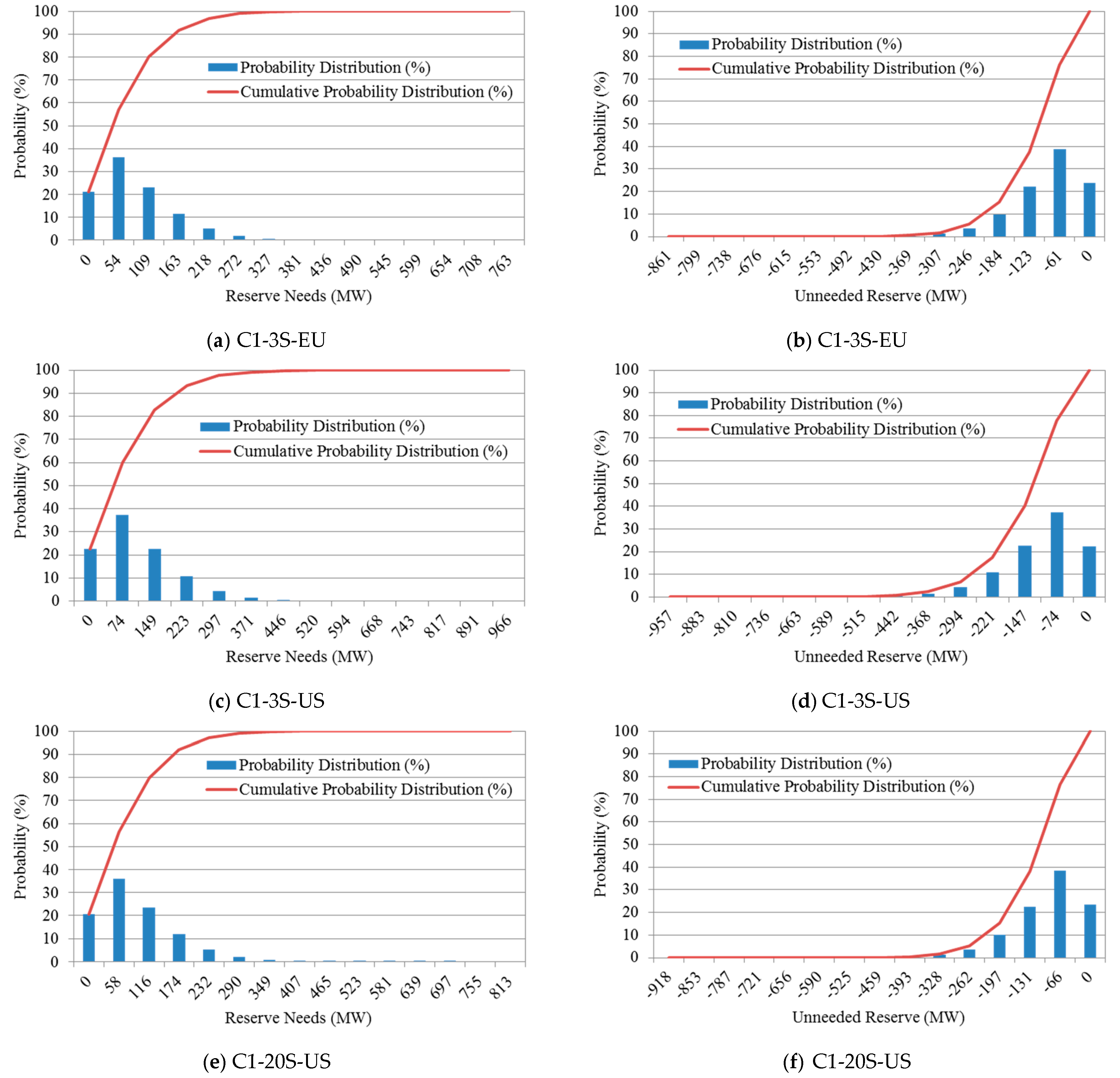
Before starting the discussion of this section, it is important to define reserve needs and unneeded reserve in this context. Reserve needs consist of, within the simulation procedure, hourly observations of the power required to cover load and wind power forecasting errors. Unneeded reserve means hourly observations of the available power scheduled to cover the secondary reserve requirement, but that are not effectively used. Figure 2 shows an example of the probability distribution functions produced to analyze the reserve needs and unneeded reserve for the C1-3S-EU case of Table 5. In general, one can interpret this case as follows: In Figure 2a, the range of the events of reserve needs varies from 0 MW to 763 MW, where the most probable events of reserve needs are between 0 MW and 272 MW. From this latter value to 763 MW, the events of reserve needs have a small probability of occurrence. In the same sense, in Figure 2b, the events of the reserve unneeded vary from −861 MW to 0 MW, where the most probable events of unneeded reserve are between −246 MW and 0 MW. From −246 MW to −861 MW, the events of unneeded reserve have a small probability of occurrence. Replacing time-series does not affect the shape of the probability distribution functions evaluated. In fact, only the range of the wind power forecasting error changes with this replacement. From Figure 2a–f, it is possible to verify the impact that this level of wind power penetration has on the total reserve needs.

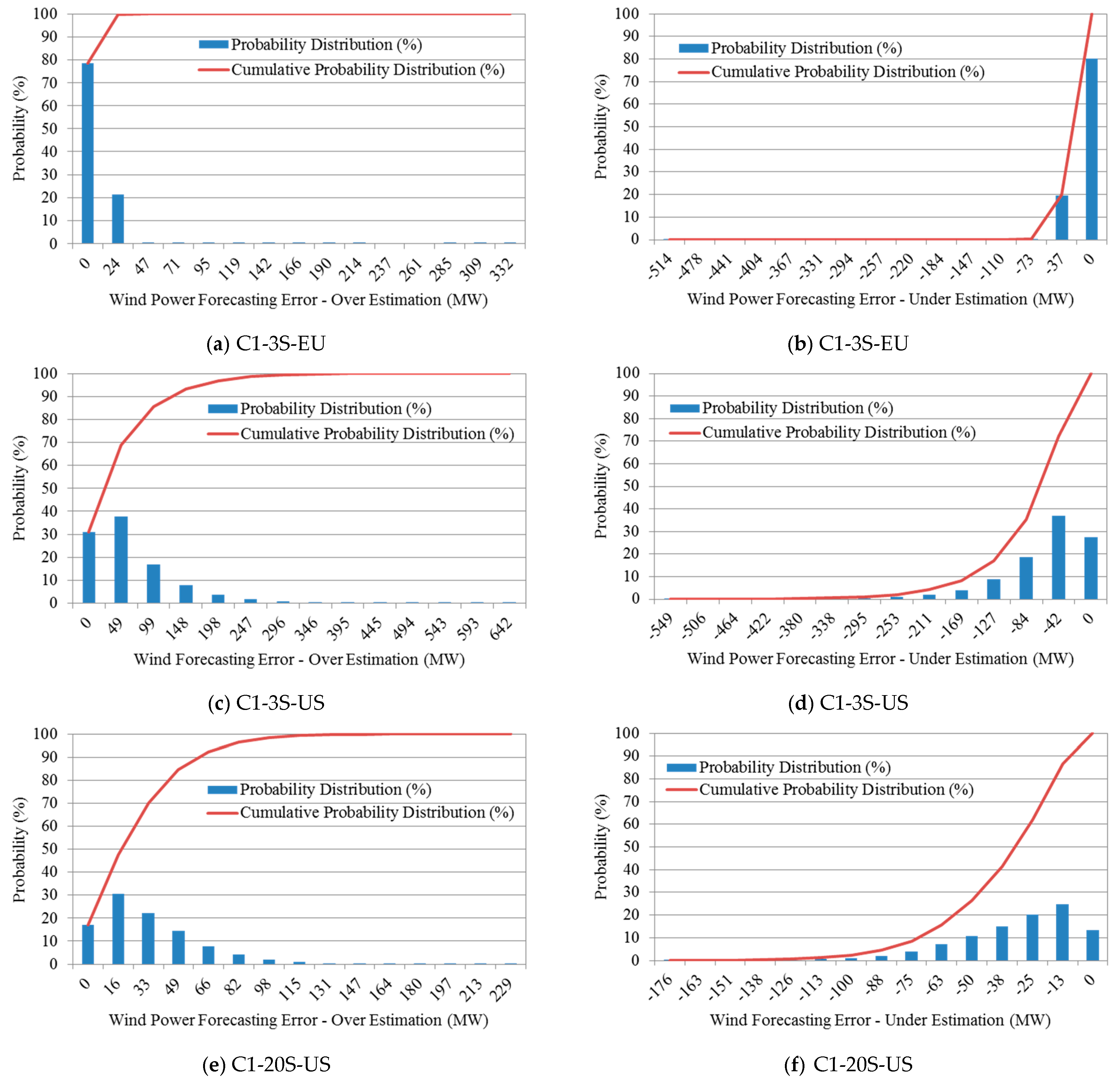
The degradation of the operating reserve capacity indices shown in Table 5 (from C1-3S-EU to C1-3S-US) can also be explained by the behavior of the wind power forecasting error. Figure 3 shows the probability distribution functions of the wind power forecasting error for the same cases in Table 5. In cases C1-3S-EU and C1-3S-US, where the level of wind power integration remains the same and the wind behavior changes, the main consequence was increasing the range of over and under estimation events during the simulation procedure. In Figure 3a–c, the over estimation events on the tail of the distribution functions have very low probabilities, increasing from 332 MW to 642 MW. In Figure 3b–d, the under-estimation events on the tail of the distribution function decrease from −514 MW to −549 MW in the same comparison. Another effect is observed through the most probable events; whereas in C1-3S-EU, the most probable events are in the interval between {0, 24} MW and {−37, 0} MW, in case C1-3S-US are in the interval between {0, 148} MW and {−127, 0} MW. The increments on reserve need to cope with the poor representation of the wind series (considering only three series) to justify the degradation of the reliability indices from the perspective of the operating reserve capacity (see Table 5). Nevertheless, Figure 3e–f highlights the importance of representing wind diversity on wind power penetration studies. The compensation effect caused by the relationship between wind farms, observed after increasing time-series from C1-3S-US to C1-20S-US, can be confirmed through the probability distribution functions of wind power forecasting errors.

The range of the most probable events in both cases decreases significantly; whereas in C1-3S-US (Figure 3c), the most probable events are inside the interval between {0, 148} MW, in case C1-20S-US (Figure 3e) are inside the interval between {0, 66} MW. This is also reflected in Table 5 through the decrease of the risk indices. Undoubtedly, the relationship between wind farms can effectively bring benefits to wind power integration.

5. Conclusions

The strong dependence of wind power on meteorological conditions creates a volatile and variable characteristic for this type of resource. Such dependence impacts on planning the integration of additional generation plants and establishing reserve requirements. This paper presents the application of operating reserve to assess geographically dispersed outputs from different wind farms considering the high uncertainty level introduced by a significant penetration of this resource.

From result analysis, simulations have shown that the increase of the number of time-series used in the wind modeling caused the increase of operating reserve capacity. The smoothing effect due to dispersed wind farms have led to a safer operation, reinforcing the expected theoretical benefit referred to as compensation of wind production. One can verify that not considering the operating constraints can lead to more optimistic reliability indices and the diversification tends to improve the reliability. By comparing cases where wind power integration increases significantly and total thermal capacity decreases, it is observed that the operating risk also increases. This highlights the importance of an adequate balance between wind and thermal generation in terms of capacity. The compensation effect caused by the geographic dispersion of wind farms has been confirmed through the estimated probability distribution functions of wind power forecasting errors. The estimated probability distribution of reserve needs also provided ranges for the most probable events of interest.

Although the idea of smoothing the variation by independent or negatively correlated outputs has been discussed in the literature earlier, this paper proposes a quantitative approach based on an operating reserve perspective. This provides two insights: First, it shows that whether we use static reserve or operating reserve calculations, the geographical dispersion is conducive to a smoother output and an improvement in reliability. The second is that the reliability may be affected by shortages due to forecast errors and forced outages. The application of wind time series in the SMCS is devised to improve adherence to reality within the simulation procedure. Also, the production of the units depends also upon the nominal capacity of the generation machines and their availability at each time instant. The impact of geographic dispersion in the reliability indices is computed in the sense that several different patterns, not necessarily directly correlated, may provide a smoothing effect in the total wind production. If a composite reliability evaluation, with transmission line representation, would be the subject of study, the simulation of time correlations for close wind farms would be strictly necessary. This will be a subject of future works alongside the representation of electrical vehicles and risk analysis.