Effects of Aerodynamic Interactions of Closely-Placed Vertical Axis Wind Turbine Pairs

Abstract

In this study, a numerical model was developed to study the effects of aerodynamic interactions between a pair of counter-rotating vertical axis wind turbines (VAWTs) in close proximity. In this model, the rotor rotation is not prescribed as a constant as in most other studies, but is determined by the moment of inertia and the total torque of the rotor, including the aerodynamic torque, generator torque, and a torque representing friction. This model enables study of the behavior of the rotor under an arbitrary ambient wind profile. The model was applied to an isolated rotor with five straight J-blades and pairs of identical rotors placed in close proximity. Compared with an isolated rotor, the aerodynamic interactions between the pair of rotors enhance the aerodynamic torques on the rotors and significantly increase the turbine power output on a per unit basis. The enhancement in turbine power output due to aerodynamic enhancement decreases with the distance between the pair of rotors.

1. Introduction

For the past few decades, development of wind turbine technology has contributed to great growth of wind energy applications. Most technology development was made on large, megawatt, horizontal-axis wind turbines (HAWTs), which are standard industry practices in wind energy utilization. Modern wind farms comprised of HAWT require significant land resources to separate each wind turbine from the adjacent turbine wakes. This aerodynamic constraint limits the amount of power that can be extracted from a given wind farm footprint. The resulting inefficiency of HAWT farms is currently compensated for by using taller wind turbines to access greater wind resources at high altitudes, but this solution comes at the expense of higher engineering costs and greater visual, acoustic, radar, and environmental impacts.

Vertical axis wind turbines (VAWT), on the other hand, provide an alternative approach in wind energy applications. VAWTs have some advantages compared with large HAWTs. For example, they are omni-directional; therefore, they do not require complex yaw-control to point into the wind. They could utilize long blades; therefore, providing a large swept area on a small footprint. Because of their small sizes, their installation, operation, and maintenance are much easier than large HAWTs, and their visual and acoustic signatures are also smaller. Because they operate at a smaller tip-speed-ratio (TSR) than HAWT, they are also safer for flying animals such as birds and bats.

VAWTs can be categorized into two major types: Savonius and Darrieus. The Savonius turbine is a drag-based turbine. The simplest design consists of a rotor made of two half cylinders. The wind faces the concave face of one cylinder and the convex face of the other. The difference in the drag forces exerted by the wind on these cylinders drives the rotation [1]. The Savonius turbine has very low aerodynamic efficiency.

The Darrieus type VAWT, on the other hand, is a wind turbine driven by lift force [2]. The Darrieus turbine consists of two or more airfoil-shaped blades attached to a rotating vertical shaft. The aerodynamic lift acting on the blades generates a torque that drives the rotation of the rotor. However, unlike the Savonius type, due to the small lift forces on the blades at low rotational speeds, sometimes the torque is insufficient to overcome the friction at startup, especially for low-solidity Darrieus VAWT when the blades are at the low-lift locations at the azimuth circle [3]. Nonetheless, the Darrieus turbines have a higher efficiency, some of them approaching that of HAWT. Most of the commercial VAWTs are of this type.

Most of the aerodynamic studies on VAWT focused on improving the efficiency of the turbines, especially that of the Darrieus type. Various blade types have been studied with the goal to improve the turbine efficiency. Early studies used NACA 4-digit symmetric airfoils (such as NACA 0015) and 6-digit cambered airfoils [4]. 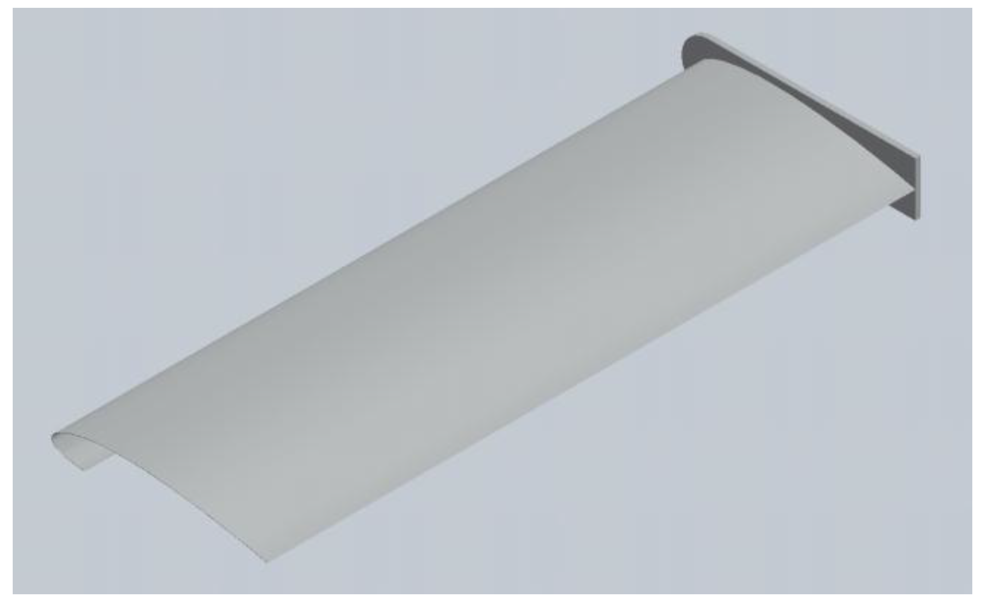Custom-designed airfoils based on the NACA series were also used on some VAWTs [5,6]. A new type of blade is the J-shaped blade (Figure 1), which assumes a hollow contour and follows most of the suction-side surface of a conventional solid blade and only the leading edge portion of the pressure-side surface. The J-shaped blade uses both lift and drag forces to drive the rotor rotation and combines both the features of Savonius and Darrieus type blades. It is demonstrated to be easier to self-start [7].

A lot of studies and effort have been made to improve the efficiency of VAWTs. Most of them focused on the efficiency of individual turbine units. A popular approach is to use pitch angle control to adjust the blade angle of attack and to reduce the aerodynamic stall effect [8]. Because the azimuthal velocity contributes to the relative wind velocity at the blade, a similar way to control the blade angle of attack is through rotor speed control [9]. The concept of a flexible blade was also explored and demonstrated to improve the blade efficiency [10]. Boundary layer actuations by mechanical or plasma actuators [11] could also improve blade efficiency. Other methods such as using a trailing edge flap [12] and auxiliary flow augmentation systems such as guided vanes [13] could also improve the efficiency.

In addition to studies focusing on individual VAWT units, recently, a new approach was developed to improve the overall efficiency of VAWT arrays or farms. The basic principle is that by placing counter-rotating VAWTs in close proximity, the aerodynamic interactions between the VAWTs could significantly enhance the power output. With the optimal placement, it is possible to produce significantly more energy per unit ground area using VAWTs instead of HAWTs [14]. Further field studies also demonstrated substantial improvement by placing VAWTs in an optimal array [15].

The aerodynamic interactions between closely-placed VAWTs have also been studied numerically by computational fluid dynamics (CFD). Giorgetti et al. [16] used ANSYS CFD to analyze the aerodynamic interferences in counter-rotating and co-rotating arrangements. Bremseth and Duraisamy [17] showed that the aerodynamic interference between turbines gives rise to regions of excess momentum between the turbines that leads to significant power augmentation. The enhanced efficiency through aerodynamic interactions was also demonstrated on Savonius type VAWT [18].

In most of the CFD studies of multiple VAWTs in the literature, the efficiency was evaluated by prescribing the rotational speed of the VAWTs, usually at the same rotational speed for all units in the array. The value of the rotational speed used at various environmental wind velocities is usually based on the optimal TSR. However, in an array setting, the rotational speeds of individual VAWTs might vary. Therefore, to understand and to more accurately assess the enhancement of efficiency on multiple VAWTs, it is desired to couple the rotation of a VAWT to the aerodynamic torque acting on it. This would allow individual VAWTs to rotate at a specific speed determined by the aerodynamic torque and the resistance load (electric load from the generator driven by the rotor, torque due to mechanical friction, etc.). In addition, because of the enhanced efficiency through aerodynamic interactions when placed in close proximity, the optimal TSR determined on isolated VAWTs might not apply and would require a revised load control to re-achieve optimal TSR. It would also require the ability to couple the rotor torque to its rotation.

In this study, a numerical model was developed to couple the aerodynamics of the VAWT to its rotation. The rotation of VAWTs is not prescribed, as in most of the CFD studies on VAWTs, but is induced by wind and also affected by the generator load profile and the friction. The model was applied to both isolated VAWTs and counter-rotating VAWT pairs with various spacing values to evaluate the effect of the aerodynamic interaction on VAWTs.

2. Methods

2.1. Governing Equations

The unsteady flow field around the VAWT is numerically simulated by employing Unsteady Reynolds-Averaged Navier-Stokes equations (URANS). The formulation applies Reynolds decomposition and takes the time-average of continuity and momentum equations for incompressible flows:

$$\begin{array}{l}\frac{\partial u_i}{\partial x_i}=0\\ \frac{\partial {\overline{u}}_i}{\partial t}+{\overline{u}}_j\frac{\partial {\overline{u}}_i}{\partial x_j}=-\frac{1}{\rho }\frac{\partial \overline{p}}{\partial x_i}+\frac{\partial }{\partial x_j}\left(\nu \frac{\partial {\overline{u}}_i}{\partial x_j}\right)+\frac{\partial {\tau }_{ij}}{\partial x_j}\end{array}$$

(1)

where ${\overline{u}}_i$ and $\overline{p}$ are averaged velocity and pressure, respectively, ρ is the density of the air and $\nu$ is the kinematic viscosity. The specific Reynolds stress is calculated as ${\tau }_{ij}=\overline{u_i^{’}{u}_j^{’}}$. The shear stress transport (SST) k-ω model [19] is used for the turbulence flow around the rotor, as it produces superior accuracy in separated flows than do standard k-ω or k-ε models [20].

In this study, the rotation of the rotor is not prescribed but induced by wind. The rotation of the rotor was coupled with the aerodynamic torque acting on it. The angular velocity of the rotor ω is calculated by

$$Id\omega /dt=T_{wind}-T_{generator}-T_{friction},$$

(2)

where I is the moment of inertia of the rotor, T_wind is the aerodynamic torque acting on all the blades, T_generator is electric load from the generator, which is set as T_generator = aω² where a is a constant, and T_friction is a small value constant representing the mechanical friction on the rotor.

2.2. Numerical Model

A high-solidity rotor with five straight J-blades was studied. For simplicity, a two-dimensional (2D) model was used, representing the cross section with the blades on a horizontal plane away from the blade tips. The blade span was 0.2D, where D is the rotor diameter. The computational domain is shown in Figure 2. A hybrid grid was used in the computational model. A structured grid was used for regions adjacent to the blades. The y+ value near the blade surface was 2. The unstructured grid was used for the rotating zone and a square region just outside the rotating zone. The outer domain used structured grids.

The boundaries of the computational simulation consisted of an inlet and an outlet in the stream-wise direction, and the far-fields in the lateral direction. A uniform velocity and zero pressure gradient were applied at the inlet. Zero velocity gradient and zero pressure were applied at the outlet. Zero-gradient conditions were applied at the far-fields. No-slip boundary condition was applied on the blades.

2.3. Numerical Approach

The numerical solver developed for this study is based on OpenFOAM library, which uses the finite volume method for the numerical simulation. The PIMPLE algorithm was used to solve the Navier-Stokes equation. The PIMPLE algorithm combines the features of the PISO algorithm (Pressure Implicit Splitting of Operators) for time dependent flows and the SIMPLE algorithm (Semi-Implicit Method for Pressure Linked Equations) that is used for steady state problems.

A moving mesh was used for the rotation of the blades. The fluid domain consisted of a circular rotating zone (the green region in Figure 2b) which enclosed the blades and shared the same axis-rotation with the blades. The outer zone (the gray region in Figure 2b) was stationary. The circular rotating zone was set to rotate with the same angular velocity as the blades. The angular acceleration of the rotor (and thus the rotating zone) was calculated from Equation (2). The angular velocity and the azimuth location were determined by integration using the trapezium rule. Since the blades rotate as a rigid body and rotate together with the surrounding mesh with the same angular velocity, there was no topological mesh change except for the entire rotation of the rotating zone/mesh as a solid body. The inner rotating zone slides on the interface with the stationary zone and parameter values (e.g., u_i and p) were interpolated and exchanged between the two zones.

2.4. Code Validation

The numerical method was applied to a NACA 0012 solid airfoil, which is widely used as a lift-based wind turbine blade, and the lift and drag coefficients at Re = 360,000 and 700,000 were compared with experiments from the literature [21,22,23]. The lift and drag coefficients for a solid NACA 0012 airfoil from the numerical simulation compare favorably with experimental measurements (Figure 3). The lift and drag coefficients of a J-shaped airfoil based on NACA 0012 were also evaluated using the CFD at Re = 700,000 and are plotted in Figure 3. The lift coefficient on a J-shaped airfoil is larger than that of a solid airfoil. Compared with the solid airfoil, the J-shaped airfoil also stalls at a slightly larger angle of attack. The drag coefficient of the J-shaped airfoil is also mostly larger than that of a solid airfoil except near α = 15 degrees, where the solid airfoil stalls but not the J-shaped airfoil.

2.5. Grid Convergence

To determine a sufficient grid size, the power coefficient for an isolated VAWT was calculated at several grid resolutions (

Table 1. Comparison of mesh refinements in power coefficient of a VAWT rotating with an angular velocity of 2π rad/s in 10 m/s ambient wind.

Grid	Number of Grid Cells	Power Coefficient
G1	62,499	0.1683
G2	137,858	0.2058
G3	265,650	0.1902
G4	501,689	0.1892

). Each grid size in Table 1 has about twice the number of the grid cells than the previous grid resolution level. The change of the power coefficient from grid G1 to G2 is 22.3%, 7.6%, and 0.5%. Therefore, the mesh G3 represents a sufficiently resolved grid and, therefore, is used in all further computations.

3. Results

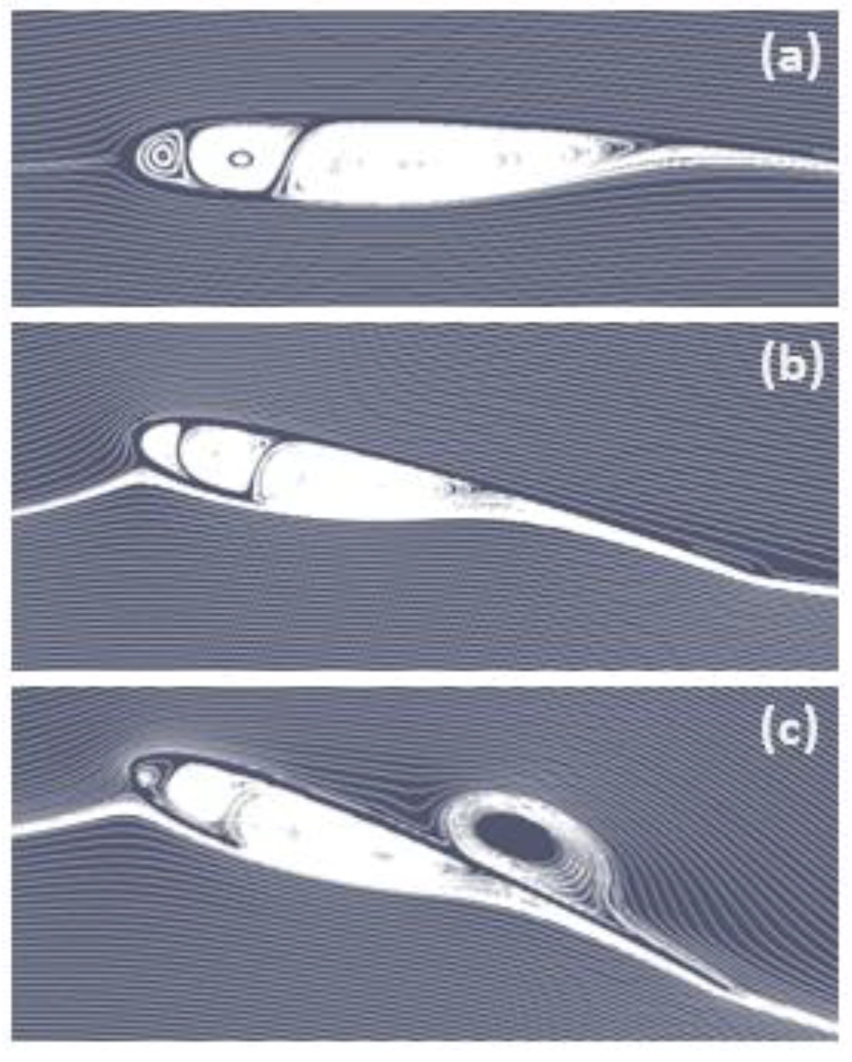
First, flow around a single J-blade at several angles of attack α was simulated at Re = 133,000. The streamlines of the flows at these angles of attack are shown in Figure 4. At α = 0, the flow is attached to the external surface of the blade. Circulations form inside the cavity of the half-close leading edge portion of the blade. Circulation also forms on the open trailing edge portion of the blade, with smooth potential flow around it as it was a solid airfoil. At α = 10°, the flow is similar to that at α = 0, with the exception of the stagnation point located downstream of the leading edge on the pressure-side surface. At α = 20°, flow separates from the suction-side surface whereas the flow on the pressure side is similar to that at lower α.

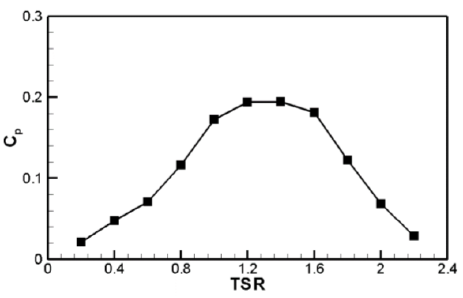
The power coefficient (C_p) versus TSR curve was determined by the conventional method of prescribing a constant TSR on the rotor and calculating the power output from the rotor, and the curve is shown in Figure 5. The power curve at various TSR values was calculated using a constant angular velocity ω = 2π rad/s and various ambient velocities. The power coefficient increases with TSR to an optimal value around 1.4, and then it begins to decrease. The low efficiency at small TSR is mostly due to stall. With a small TSR, the angle of attack on a rotating blade is larger where stall would occur. At a large TSR, the low efficiency is mostly due to the drag on the blade. The optimal TSR is considered smaller than that of solid-blade rotors because the J-blade design combines the features of Savonius type (low designed TSR) and Darrieus type (high designed TSR) turbines. The overall power coefficient values for the turbine are relatively low compared with the theoretical Betz’s limit of a wind turbine (59.3%) due to several reasons. First, the power efficiency for VAWTs is generally lower than that of HAWTs. In addition, the high solidity of the rotor (σ = 1 for the 5-blade rotor) also causes the power efficiency to be low.

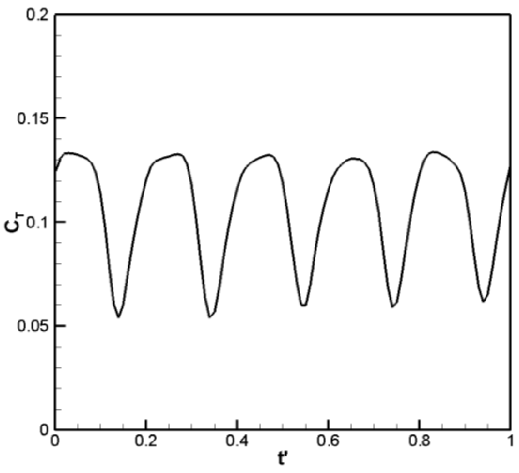
The evolution of the aerodynamic torque on the rotor with respect to azimuth angle during one revolution of the rotor is shown in Figure 6. Because there are five blades on the rotor, the torque shows five oscillations within one revolution of the rotor. The oscillation of the torque is the source of the transient load on the blade.

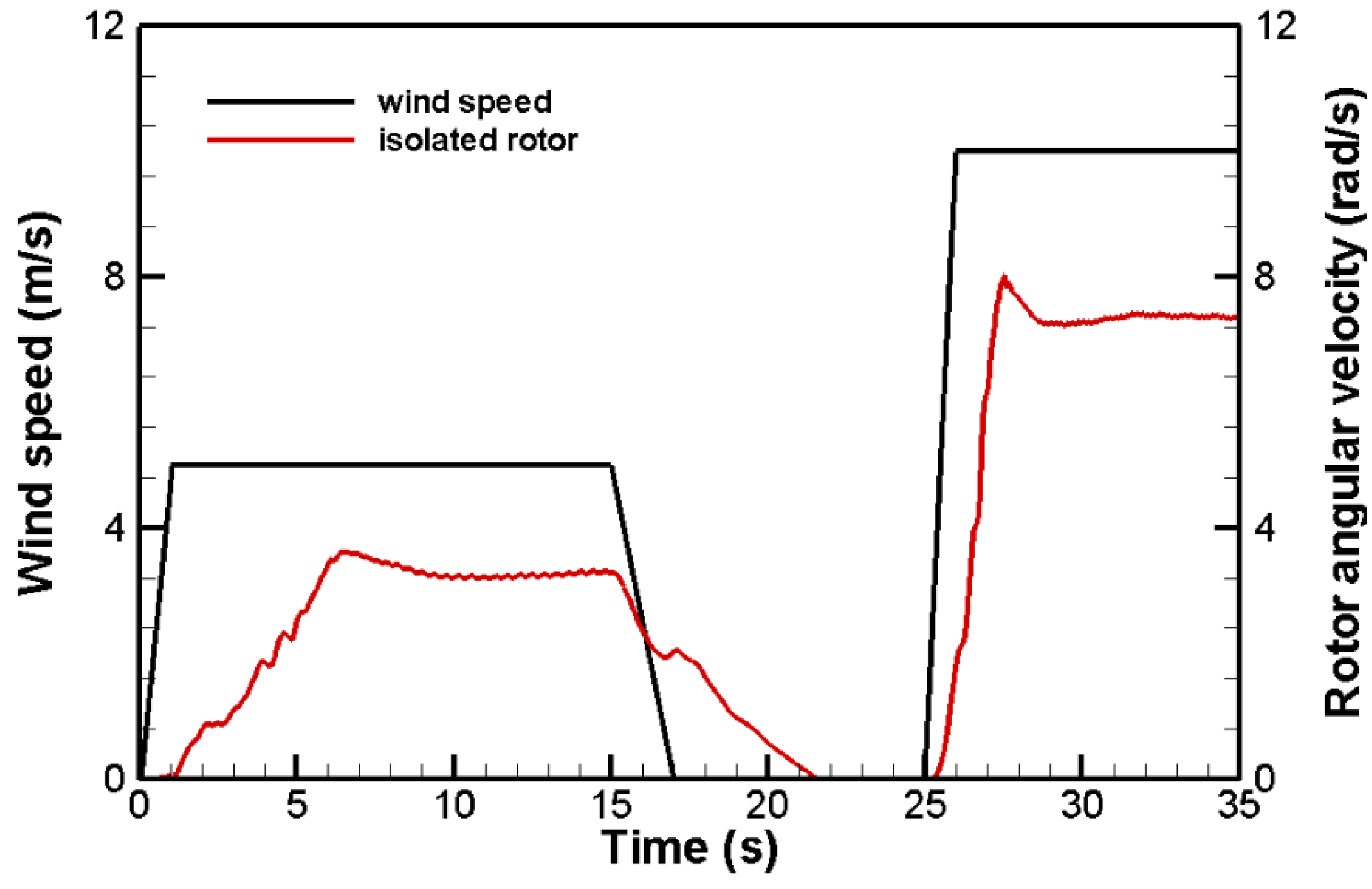
Compared with most CFD models of VAWTs where the rotor rotation speed is prescribed, one new feature of the model presented in this study is that the rotor ration is induced by the ambient wind. This allows for study of the behavior of the rotor in response to an arbitrary ambient wind profile. It also enables evaluation of the enhancement of the induced rotation speed and the power generation on a rotor pair. Therefore, instead of applying a constant wind velocity, the wind-induced rotation of the rotor was studied on VAWTs under a variable ambient wind velocity profile, which was applied as the uniform boundary condition at the inlet:

$$u\left(t\right)=\{\begin{array}{c}\begin{array}{cc}5t\mathrm{m}/\mathrm{s},& for0<t\le 1\mathrm{s}\\ 5\mathrm{m}/\mathrm{s},& for1<t\le 15s\\ 5-2.5\ast \left(t-15\right)\mathrm{m}/\mathrm{s},& for15<t\le 17\mathrm{s}\end{array}\\ \begin{array}{cc}0,& for17<t\le 25\mathrm{s}\\ 10\left(t-25\right)\mathrm{m}/\mathrm{s},& for25<t\le 26\mathrm{s}\\ 10\mathrm{m}/\mathrm{s},& for26<t\le 35\mathrm{s}\end{array}\end{array}$$

(3)

The ambient wind velocity is shown in black in Figure 7. The wind profile consists of plateaus of constant wind speeds, with ramp-up and ramp-down between these wind speeds. First, the ambient wind velocity linearly ramps up from u = 0 at t = 0 to u = 5 m/s at t = 1 s. The ramp-up in wind speed would demonstrate the start-up behavior of the VAWT. The wind speed then stays a constant at u = 5 m/s from t = 1 s to t = 15 s. This wind speed of 5m/s was used because it is about the average annual wind velocity at 10 m hub height at a class 3 wind site, which is the design target for a small (e.g., 2 kW) VAWT. The wind speed then linearly ramps down to u = 0 at t = 17 s and stays at u = 0 until t = 25 s. The ramp-down in wind speed to u = 0 would demonstrate the slow-down of the VAWT to still. The wind speed then linearly increases to u = 10 m/s at t = 25 s and stays a constant to demonstrate the response of VAWT to a larger wind speed value. The variable wind velocity profile in Equation (3) was used to demonstrate that the rotor is able to start from still, to ramp up to angular velocity, and to slow down when wind velocity decreases. The rotor angular velocity varies in response to the total torque acting on the rotor, which consists of the aerodynamic torque T_wind, the generator load torque T_generator = aω² (where a = 0.5 N·m·s²), and the constant mechanical friction torque T_friction = 10 N·m.

The induced angular velocity of an isolated rotor ω under this environmental wind profile is shown in red in Figure 7. The initial angular velocity of the rotor is ω = 0. It then slowly ramps up to about ω = 3.6 rad/s at about t = 6 s. Then, it slows down a little bit to reach a steady-state rotation at about ω = 3.2 rad/s. The small over-speeding of the rotor before it reaches the steady state is mostly due to the inertia of the rotor. At t = 15 s, rotor angular velocity ω starts to decrease as the wind slows down. Even though wind velocity becomes u = 0 at t = 17 s, ω does not reduce to 0 until about t = 21.5 s because of the rotor inertia. At t = 10 s, the wind ramps up again to u = 10 m/s and ω starts to increase. It over-speeds to ω = 8.0 rad/s before reducing to the steady-state rotation of ω = 7.3 rad/s.

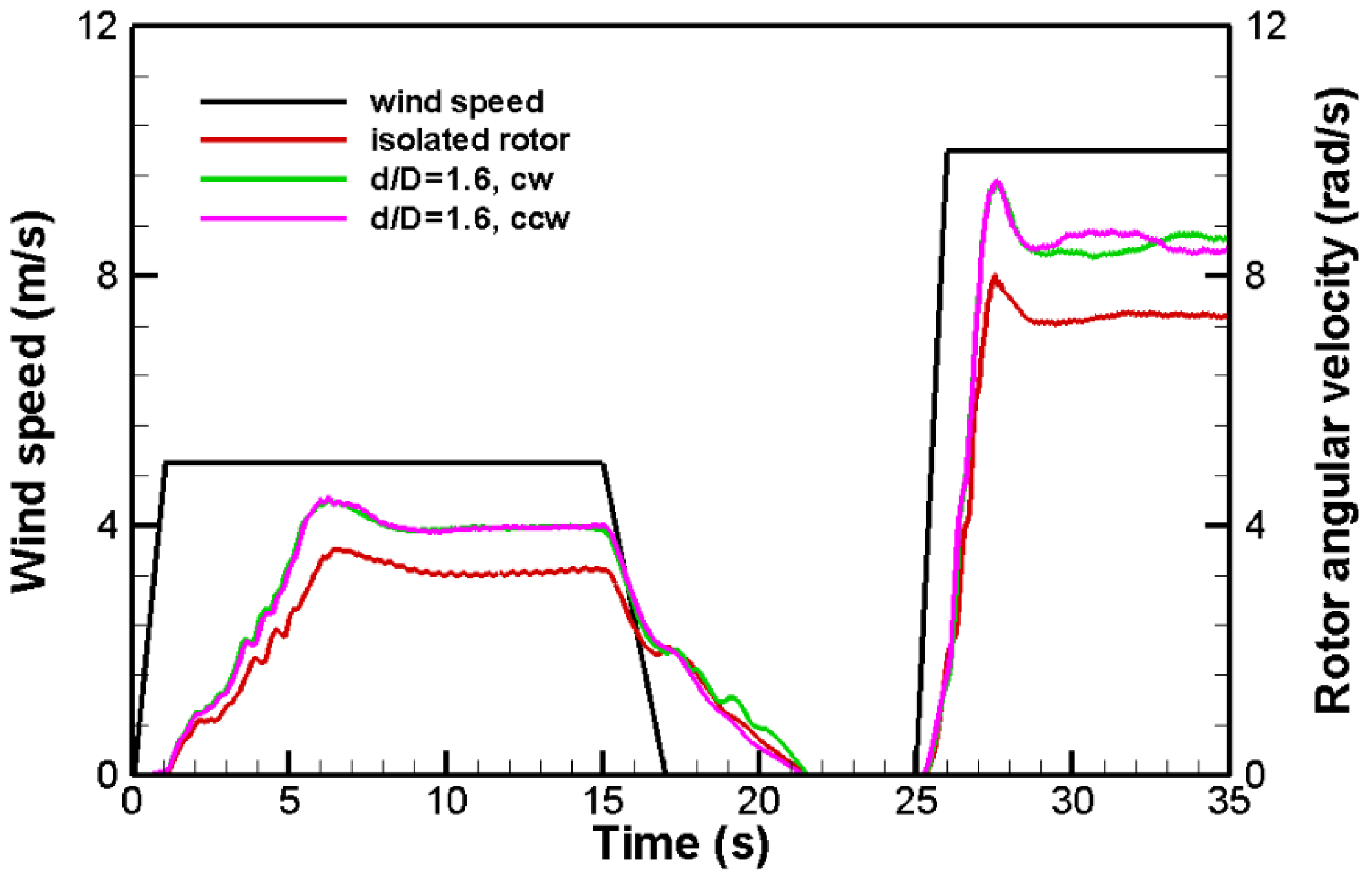
The same ambient wind profile was also applied to a pair of counter-rotating VAWTs with pole-to-pole distance d = 1.6D, where D is the rotor diameter. The two VAWTs in the pair are configured in an opposite direction of rotation. The angular velocities for the two rotors, in response to this environmental wind profile, are shown in Figure 8. In addition, the angular velocity of an isolated rotor under the same wind profile is shown in Figure 8 as a comparison. The rotation of the pair of rotors behaves similarly under the wind as does the isolated rotor, as their angular velocities evolve similarly to wind as that of the isolated rotor. However, the paired rotors rotate faster than the isolated rotor at the same ambient wind speed. For example, at the ambient wind velocity of u = 5 m/s, the steady-state rotation speed for the isolated rotor is about ω = 3.2 rad/s, whereas for the paired rotors, the angular velocities is about ω = 4 rad/s, an increase of about 25% in rotor speed. The paired rotors also ramp up faster than the isolated rotor from still.

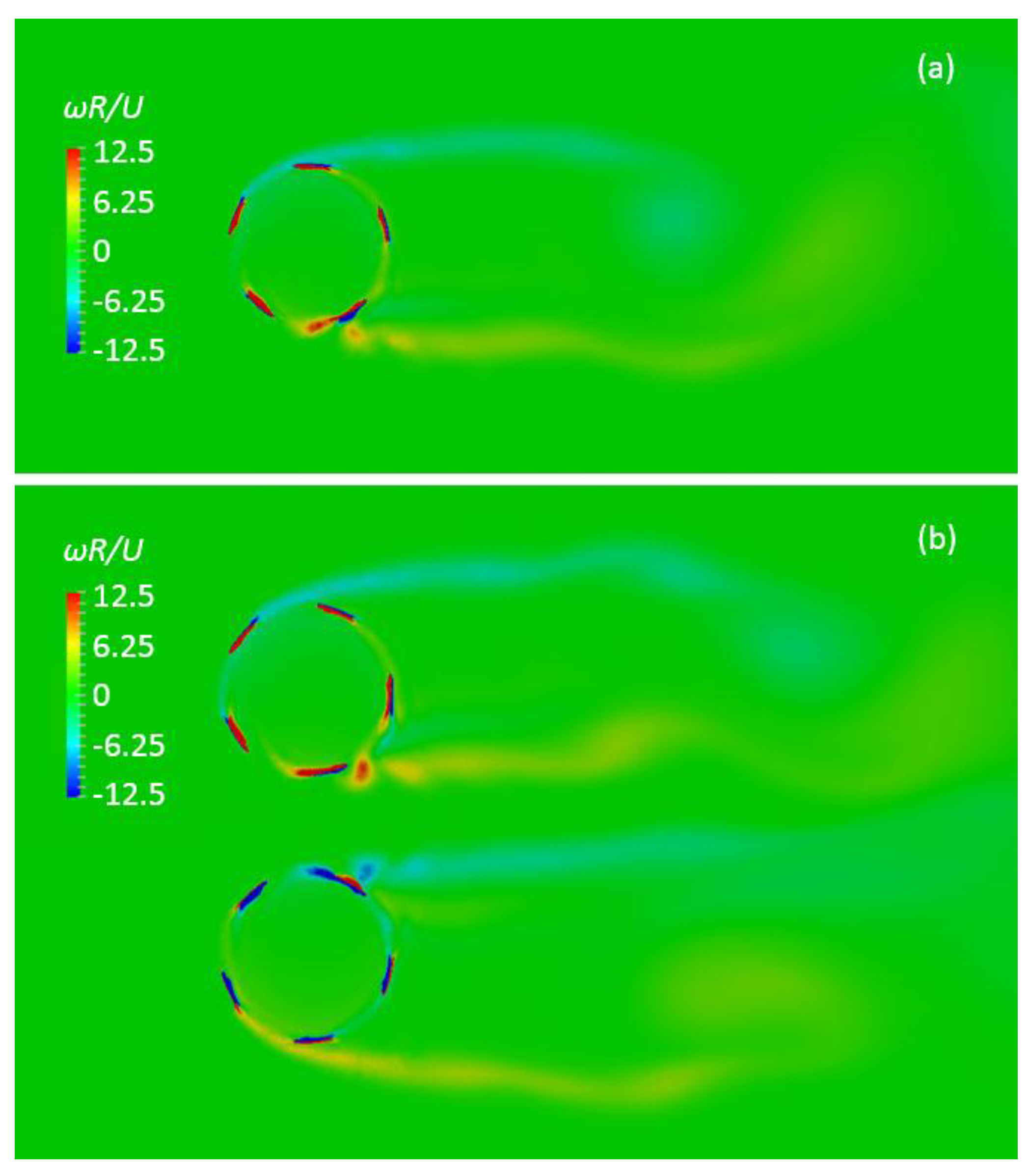
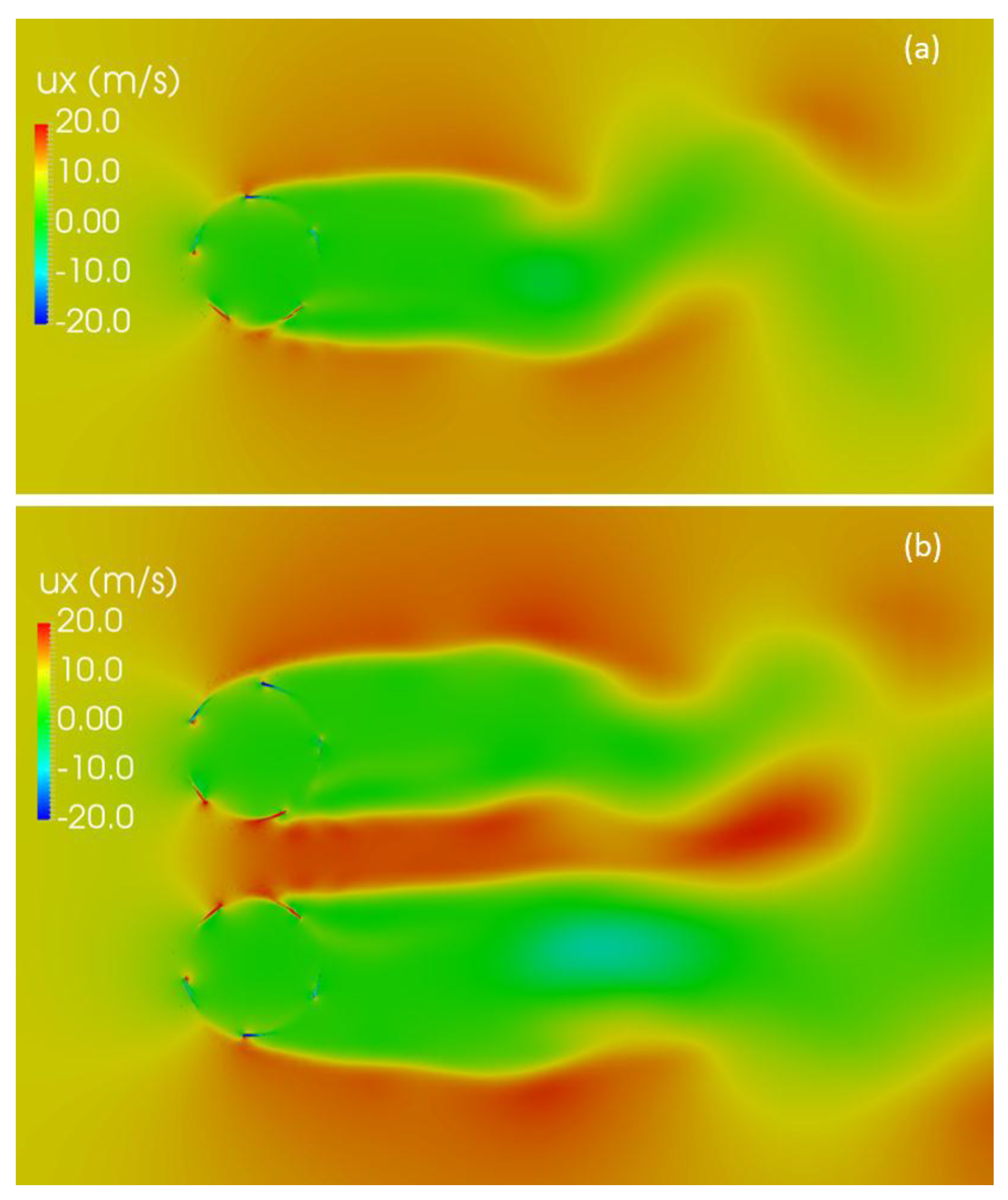
Flow vorticity fields were also compared between an isolated rotor and a pair of rotors. Snapshots of the vorticity fields generated by an isolated rotor and a pair of rotors are shown in Figure 9. Both are steady-state rotations with ambient velocity u = 10 m/s. The vorticity near the blades are higher in the pair rotors than that in the isolated rotor, from the higher rotational speeds of the paired rotors. The overall flow of the paired rotors behaves like a counter-rotating vortex pair, and as pointed out by a previous study [15], this flow pattern increases stream-wise flow speed between the two rotors (Figure 10), which is the main mechanism of the increased aerodynamic performance and power output on a pair of counter-rotating VAWTs in close proximity.

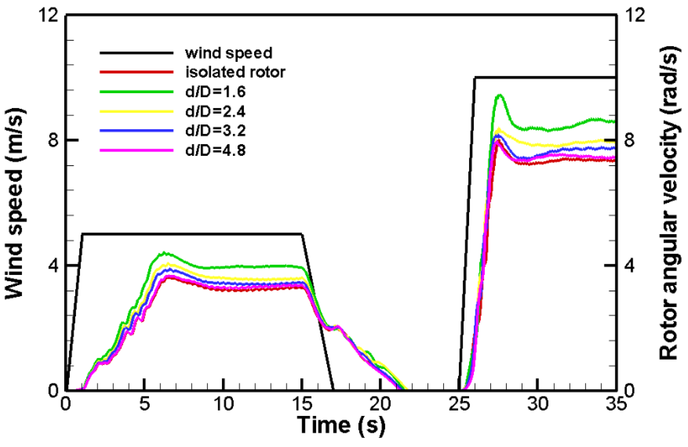
The same ambient wind profile was also applied to pairs of counter-rotating VAWTs with various pole-to-pole distances. The angular velocities of the rotors with pole-to-pole distances at d/D = 1.6, 2.4, 3.6, and 4.8 are shown in Figure 11, in addition to that of an isolated rotor. Because the angular velocities for the two rotors in the same pair configuration behave similarly (demonstrated in Figure 8 at d/D = 1.6), only the angular velocities of the clock-wise rotors in the pairs are shown in Figure 11. The angular velocities of the paired rotors behave similarly under the same wind profile. For paired rotors at each spacing configuration, ω is higher than that of an isolated rotor. The larger the spacing between the paired rotors, the smaller the aerodynamic enhancement as ω approaches that of an isolated rotor.

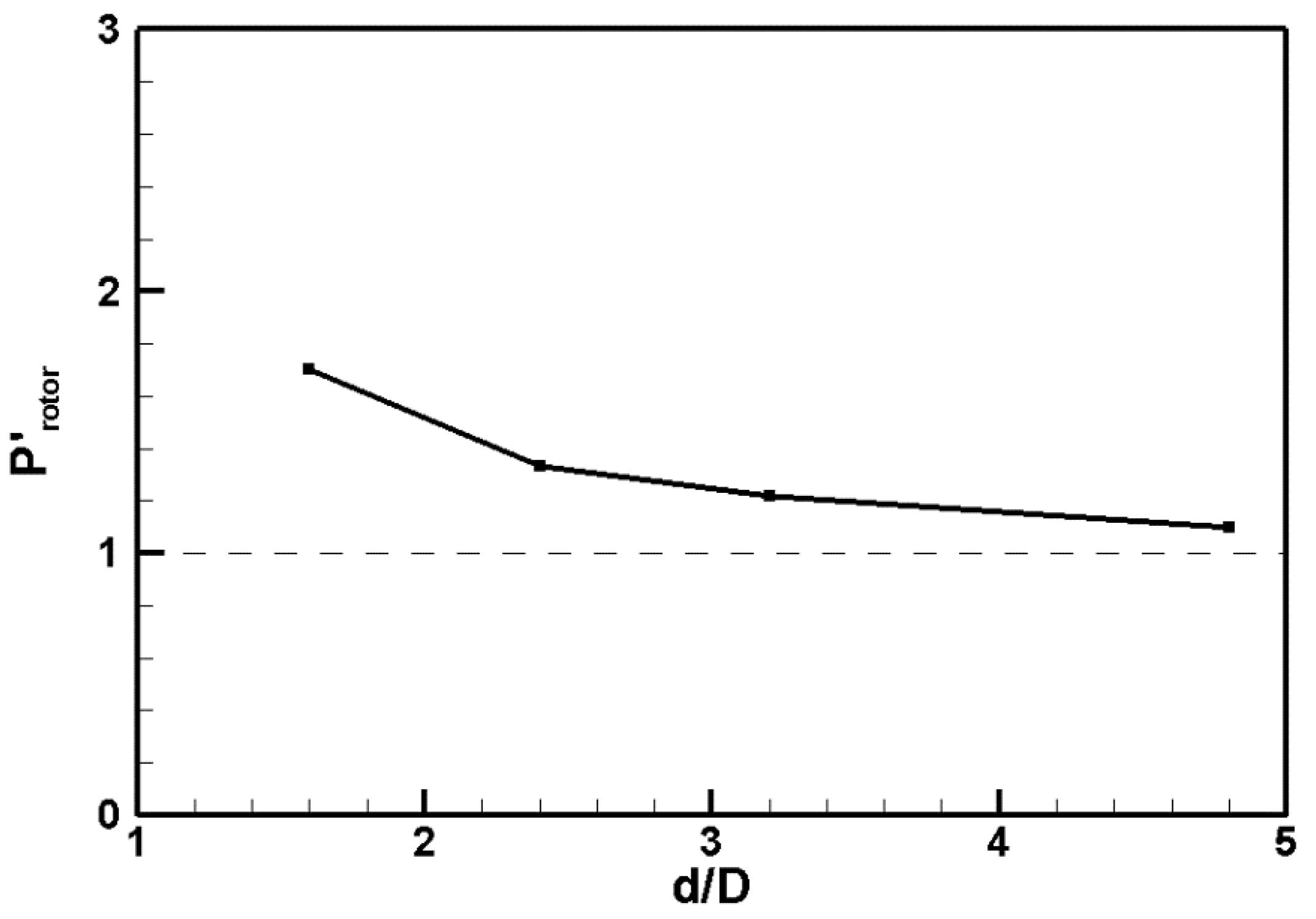
The aerodynamic enhancement has been demonstrated in the angular velocity of the paired rotors. The benefits in power output from the turbine generator were also evaluated. Because the generator load torque profile was set as T_generator = aω², which was applied on the rotor as a resistance torque in the simulation of the wind-induced rotation, the power output of the generator can be calculated as P = aω³. The time-averaged power output was calculated for paired rotors with various pole-to-pole distances. The power output was then normalized by the time-averaged power output of the isolated rotor and is plotted in Figure 12. Note that the averaged power output for paired rotors shown in Figure 12 is evaluated on the per rotor basis. At a pair of rotors at d/D = 1.6, the average power output per rotor is about 70% more of that of an isolated rotor, which is a significant improvement in power output due to aerodynamic interactions. With an increasing spacing between the paired rotors, the power output decreases due to less aerodynamic enhancement effect.

4. Conclusions

In this study, a numerical model was developed to study the effects of aerodynamic interaction between a pair of counter-rotating VAWTs in close proximity. In this new approach, the aerodynamics of wind turbine rotors are coupled with their rotational dynamics. Therefore, the rotor rotation is induced by wind, not prescribed as a constant as in most of other studies. The rotational dynamics of the rotor is determined by the rotor moment of inertia and the total torque on the rotor, including the aerodynamic torque, generator torque, and a torque representing the friction.

The rotational behavior of the VAWT follows that of the ambient wind conditions. When wind picks up, the rotor responds with an increased angular velocity. When wind increases to a constant, the rotor would over-speed a little before setting on a relatively steady-state rotational speed due to the rotor inertia. When wind velocity decreases, the rotor angular velocity would also reduce, though more slowly than the change in wind speed, also due to the rotor inertia.

When two counter-rotating VAWTs are placed in close proximity, the aerodynamic interactions between the pair of rotors enhance the aerodynamic torques on the rotors compared with that on an isolated rotor. The increased driving torques in turn make the rotors rotate at a high angular velocity ω than does an isolated rotor. Because the generator power output P is proportional to ω³, there is significantly more power output per turbine unit from a closely-placed pair of rotors than from an isolated rotor. The enhancement in turbine power output due to aerodynamic enhancement decreases with the pair spacing between the pair of rotors.

Further study would focus on a VAWT array with multiple turbine units. The method could be used to study the effect on array configuration on the turbine rotational speed and power output. In addition, because of the enhanced efficiency through aerodynamic interactions shifts the optimal TSR, further studies could use this method to design array-specific generator load curves for a given array configuration.