Article

Numerical Modelling of Ice-Covered Insulator Flashover: The Influence of Arc Velocity and Arc Propagation Criteria

Modelling and Diagnostic of Electrical Power Network Equipment Laboratory (MODELE), University of Quebec in Chicoutimi, Chicoutimi, QC G7H 2B1, Canada
*
Author to whom correspondence should be addressed.
Energies 2018, 11(10), 2807; https://doi.org/10.3390/en11102807
Submission received: 10 September 2018 / Revised: 11 October 2018 / Accepted: 16 October 2018 / Published: 18 October 2018
(This article belongs to the Section F: Electrical Engineering)

Abstract

:
This paper investigates the influence of arc velocity and propagation criteria on the parameters of a dynamic numerical mono-arc model used to predict flashover voltage of ice-covered insulators. For that purpose, a generic algorithm has been developed which, coupled with a Finite Element commercial software, permits us to solve the mono-arc Obenaus equation. The versatility of the proposed algorithm allows to implement three different arc propagation criteria and five different arc velocity criteria, as well as to compute the corresponding flashover voltage, arc velocity and leakage current. Moreover, this algorithm permits to propose a new arc velocity criterion based on numerical calculation instead of analytical formulation as proposed in literature.

1. Introduction

Flashover on outdoor insulation caused by atmospheric icing and consequent power outages caused by contaminated ice or snow has been reported by a number of researchers around the world over the last five decades [1,2,3,4,5,6,7,8,9,10,11]. A lot of laboratory research has also been conducted on this subject [1,2,3,7,8,11]. As a general rule, these reports and studies indicate that the thickness and type of ice, the level of contamination, and the rise in air temperature have significant effects on the withstand voltage of ice-covered insulators. However, several studies in laboratory and on natural sites have reported that ice deposits formed under wet conditions are more detrimental than wet snow, cold fog and even ice formed under dry conditions [2,3,4,7,8]. According to most of these reports and observations, the number of single-phase faults increases substantially after wet grown-ice accretion when followed by a rise in air temperature. This is principally due to the presence of a conductive water film on the melting ice surface causing large voltage drops across the air gaps (parts of the insulator without ice) [12,13]. The initiation of corona discharges and the consequent development of local arcs at these sections of the insulators sometimes lead to flashover, and consequent power outages [2,8].
Under such severe atmospheric conditions, external insulation design with regard to pollution and icing performance has become a critical factor for the reliability of overhead electrical lines [5]. In order to help with the design and dimensioning of insulators dedicated to cold regions, several mathematical models to predict ice-covered insulator critical flashover voltage (FOV) were proposed in the last decades [14,15,16,17,18,19,20]. Both static [14,15,16] and dynamic [17,18,19,20] models have been used to simulate flashovers on insulators that are fully bridged by ice accumulation. However, these models do not take into account the physical mechanisms involved during the arc propagation, which is a complex phenomenon that principally depends on thermodynamic processes [21,22], electrical forces [23,24] and other mechanisms of arc propagation [25,26,27,28]. On the other hand, the discharge nature of the electrical arc propagating during flashover is dependent on the conductive layer resistivity and the geometrical parameters, as demonstrated by several authors [24,26,27,28,29]. According to these authors, the kind of discharge can be considered as a spark/leader surface discharge [28,29] or an abnormal transient glow discharge [24,26,27] with a temperature range between 1000 °K and 4000 °K [30,31,32]. These considerations have led to the development of several analytical criteria with regards to the arc propagation and arc velocity used in different mathematical static and dynamic predictive models.
The static model is concerned with finding the characteristics of the arc at its critical length leading to flashover. It has been successfully applied to short insulator strings [14,15] and, more recently, has been extended to full scale Extra-High-Voltage (EHV) post insulators [16]. In contrast, the dynamic model considers the arc as time-dependent impedance and simulates flashover development by steps [17,18,19,20]. Both models can predict the critical flashover voltage but the dynamic model can also predict leakage current during the flashover process.
Most of these predictive models proposed are based on the Obenaus/Rizk general approach initially developed for polluted insulators where a single arc is in series with a residual electrical resistance R(x), thus modelling the ice surface not bridged by the arc, as illustrated in Figure 1 and by Equation (1) [30]:
V m = x E a r c + I m R ( x ) + V e
where Vm is the applied voltage (V), x is the local arc length (m); Im is the leakage current (A), R(x) is the residual resistance of ice layer (Ω), and Ve is the electrode voltage drop and Earc is the electric field along the arc. The latter given by the following equation:
E a r c = A I m n
with A and n being the arc constants.
The major problem with these models is that the residual resistance calculation, which takes into account the arc root, is calculated from the analytical formulation proposed by Wilkins [26], expressed as follows for an ice-covered insulator [14]:
R ( x ) = 1 2 π γ e [ 4 ( L x ) D + 2 d + l n ( D + 2 d 4 r ) ]
where γe is the surface conductivity of the ice layer (µS); L and D are the arcing distance and diameter of the insulator (m), d is the thickness of the ice layer (m) and r is the arc root radius (m).
The use of Equation (3) requires the presence of a well-defined uniform ice layer that can only be obtained under severe icing conditions [14,15,16,17,18,19,20]. Under these specific conditions, the insulator is totally bridged by the ice deposit, which can then be modelled as a half-cylinder [14]. Consequently, such residual resistance formulation is difficult to adapt to non-uniform ice or insulator with complex geometries.
Another limitation regarding mathematical predictive models comes from the rigidity of these models and particularly the dynamic models that are built around a specific criterion of propagation and arc velocity [17,18,19,20]. These criteria are used to verify the condition of arc propagation and calculate the arc velocity during flashover process. On the other hand, Equations (1) and (3) are used to calculate the leakage current Im flowing in the arc in series with the ice layer (see Figure 1) as a function of applied voltage Vm. The mathematical resolution of Equation (1) is complex as it requires specific computational iterations in order to determine Im for each applied voltage Vm and the position of the arc root or arc length. Moreover, for each arc length and Im value, the arc propagation criterion and arc velocity must be determined, which increases the complexity of the calculation. This explains why such mathematical models are so rigid and necessitate the use of specific algorithms developed for each criteria used.
In order to overcome restrictions of mathematical models in terms of residual resistance calculation for complex geometries, a new predictive mono-arc model based on numerical methods was proposed during the last years [33,34,35]. Developed for determine ice-covered insulator FOV, this model uses Finite Element Method (FEM) to compute the residual resistance R(x) in series with the arc as well as the leakage current Im and the average E-field at the ice surface (inside the water film layer) in order to solve the Obenaus flashover Equation (1). Average E-field Eavg is also used to verify the arc root propagation condition based on the Hampton criterion, which is expressed as follows [36]:
E a r c < E a v g
where Eavg is average E-field inside the pollution layer.
The proposed mono-arc model takes into account the presence of the arc root, modelled as a circular equipotential surface of radius r. This assumption is based on the Wilkins hypothesis where the electrical arc is modelled as a cylinder of constant radius r (cm) given by the following equation [24]:
r = I m B π
where Im is the arc current and B is a constant that is dependent on the nature and polarity of applied voltage [26].
The FOV results obtained with the initial numerical predictive mono-arc model demonstrated very good accuracy compared to other ice-covered mathematical flashover models [33]. More recently, this numerical model was improved by implementing an arc velocity criterion based on the Gallimberti formulation [35] used in several mathematical predictive models dedicated to polluted and ice-covered insulators. With this implementation, the new dynamic numerical mono-arc model has provided more accurate FOV results for both ice-covered and polluted insulators [26,27]. However, as this dynamic mono-arc model was developed around two unique criteria of arc propagation (Hampton) and arc velocity (Gallimberti), it becomes difficult to evaluate the stability of the calculation algorithm and its accuracy regarding the choice of other criteria available in the literature. In this context, this paper presents a thorough investigation on the influence of arc velocity and arc propagation criteria of the predictive results obtained with a numerical dynamic mono-arc model. For that purpose, a generic mono-arc calculation algorithm based on the Obenaus mono-arc concept (Equation (1)) is proposed here. Coupled with FEM calculation, this generic algorithm permits to implement several arc and velocity arc criteria in order to determine the numerical stability of the algorithm as well as the influence of these different criteria on the predictive results in terms of FOV, arc velocity and leakage current obtained for different ice-covered insulators. Finally, a new formulation of the arc velocity criterion based on numerical calculation was developed and implemented in order to be applicable to complex geometries, which would be impossible with the actual analytical formulations available in the literature.

2. Presentation of the Mono-Arc Numerical FEM Model

2.1. Assumptions Used for Numerical Modelling

In order to compare the results of the proposed numerical predictive model to the results obtained from the mathematical ones, several assumptions have been made. As concerns the first assumption, the ice layer covered the windward side of the insulator is assumed to be uniform with the presence of one air gap closed to the HV electrode, as illustrated in Figure 2a,b. As a result, the ice layer can then be developed and modelled as a perfect cylinder, as presented in Figure 2b, where D is the insulator outer shed diameter, d is the ice layer thickness, L is the arcing distance and x is the arc length. With this rectangular ice layer geometry, Equation (3) can be used for residual resistance calculation, as done by the mathematical predictive models.
As for the second assumption, both mathematical and numerical FEM model are applied at the last stage of the flashover process where one partial arc is established along the unique air gap close to the HV electrode (Figure 2b). In this case, the Obenaus model of Figure 1, described by Equation (1), can be used. For the third assumption, the water film present at the ice surface is considered as a uniform and constant thin conductive surface in which all the leakage current density flows, as explained in detail in [33]. In this way, the problem is solved in 2D where only the conductive surface of the ice layer is taken into account, which is then discretized by finite elements, as shown in Figure 2c. The conductivity of the conductive surface can be expressed as follows [14]:
σ s = α σ + β
where α and β are constants depending on the nature and polarity of the applied voltage, which was determined experimentally in previous studies [14,15], and where σ is the conductivity of the freezing water used to form the ice.
Finally, for the fourth and last assumption, the partial arc, established between the HV electrode and the ice surface (Figure 2b), is considered to be modelled by its arc root of radius given by Equation (9) in contact with the 2D conductive surface, as presented in Figure 2c. The arc root is thus considered as an equipotential surface in the FEM model with a potential boundary condition, Vap, given by the following equation:
V a p = I m R ( x ) = V m x A I m n V e

2.2. Subsection Presentation of the Calculation Algorithm

In order to compute the critical FOV of the ice-covered insulator, the single-arc dynamic FEM model proposed in this study has to solve Equation (1) for DC as it is based on the single-arc Obenaus/Rizk model. For AC, however, the local arc of Figure 2b is established after Vm has reached the value corresponding to the arc re-ignition condition given by Equation (8), which must also be taken into account in the AC model. This leads to arc extinguishment and re-ignition twice in each cycle, as explained in [30] using the following equation:
V m = k x I m b
where k and b are the arc re-ignition constants.
This problem can be handled by combining the commercial multi-physics software COMSOL Multiphysics® (Version 5.2, COMSOL Inc., Burlington, MA, USA), implementing the FEM, with a general mathematical package Matlab® (Version 2017, MathWorks, Natick, MA, USA), for the calculation algorithm. FEM software COMSOL Multiphysics® is used to compute the residual resistance R(x), the peak value of the leakage current Im and the average electric field Eavg in the conductive ice surface layer for a peak value of source voltage Vm. Figure 3 presents the flowchart of the calculation algorithm implemented with Matlab®.
During the development of the calculation algorithm, special attention was paid to propose a generic mono-arc dynamic predictive model of FOV. As a result, the proposed algorithm can be used both in AC or DC voltage independently of the propagation and arc velocity implemented. In this way, the influence of these criteria on the FOV results can be studied as well as the interaction between each of them. Moreover, in order to propose a generic model, the proposed algorithm can be applied to all type of insulator geometries thanks to the implementation of the 2D open model block based on the open model method proposed by Rumeli for polluted insulators [37,38]. The open model was initially used to develop the surface geometry of a real uniform polluted insulator into an equivalent surface in 2D.

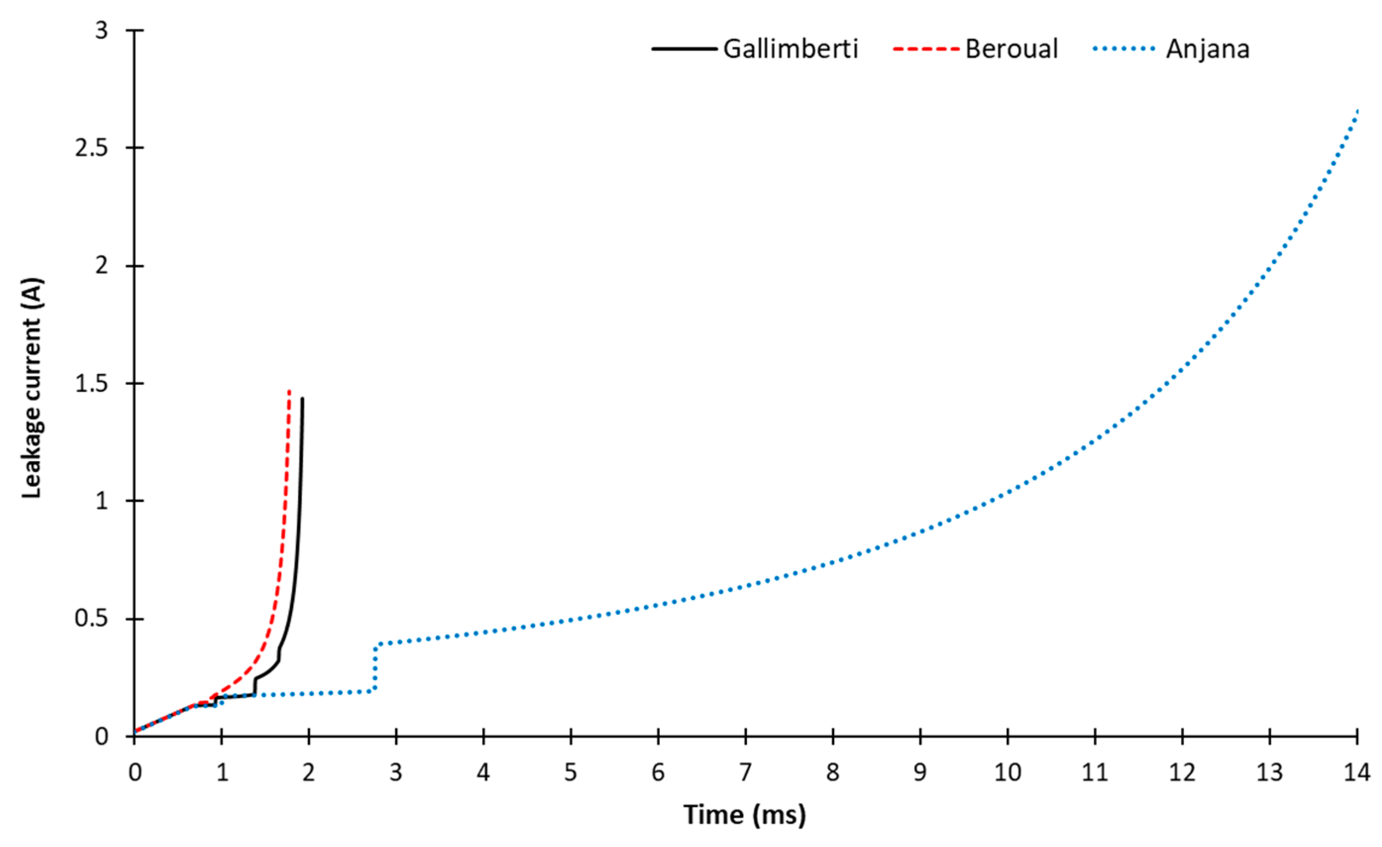
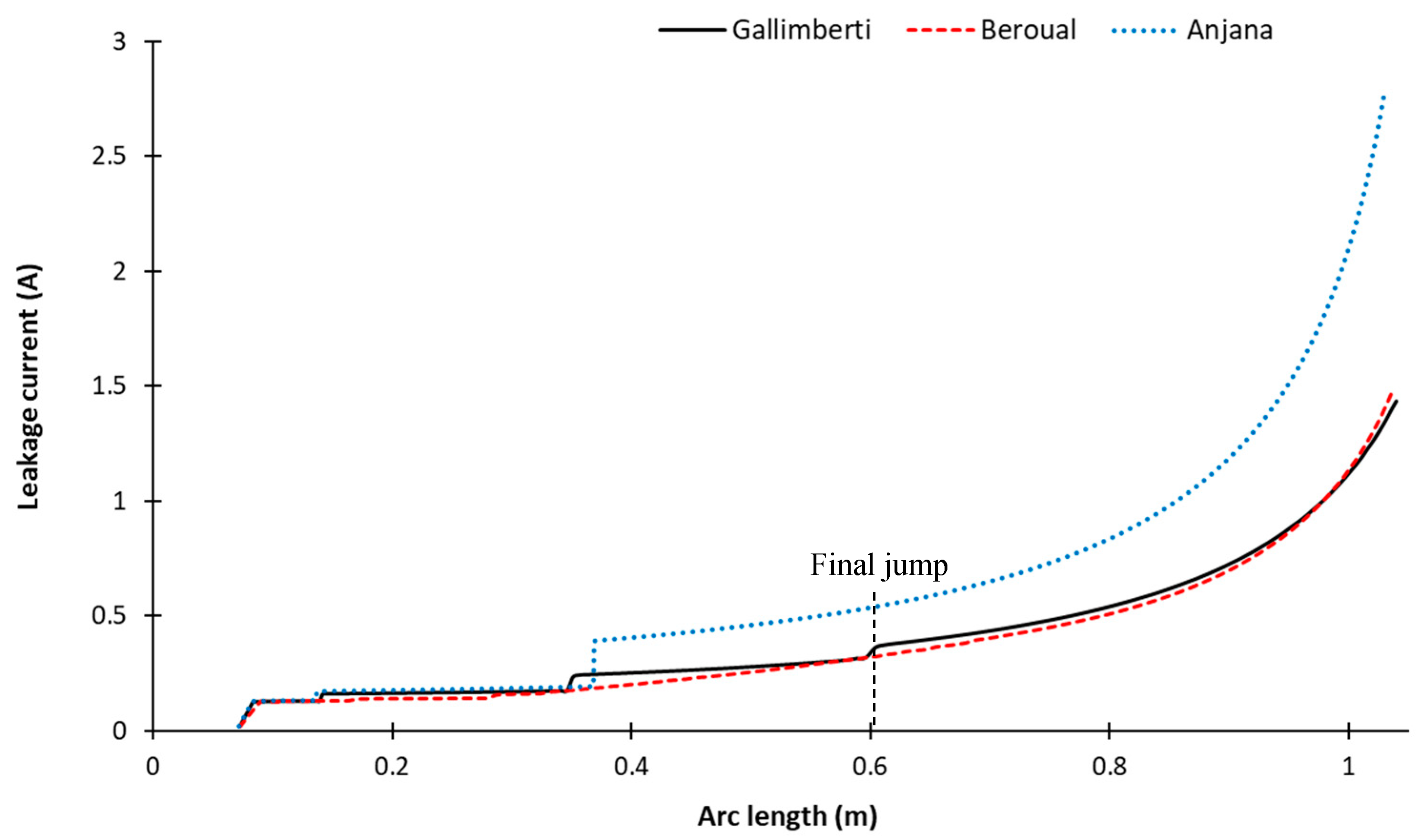
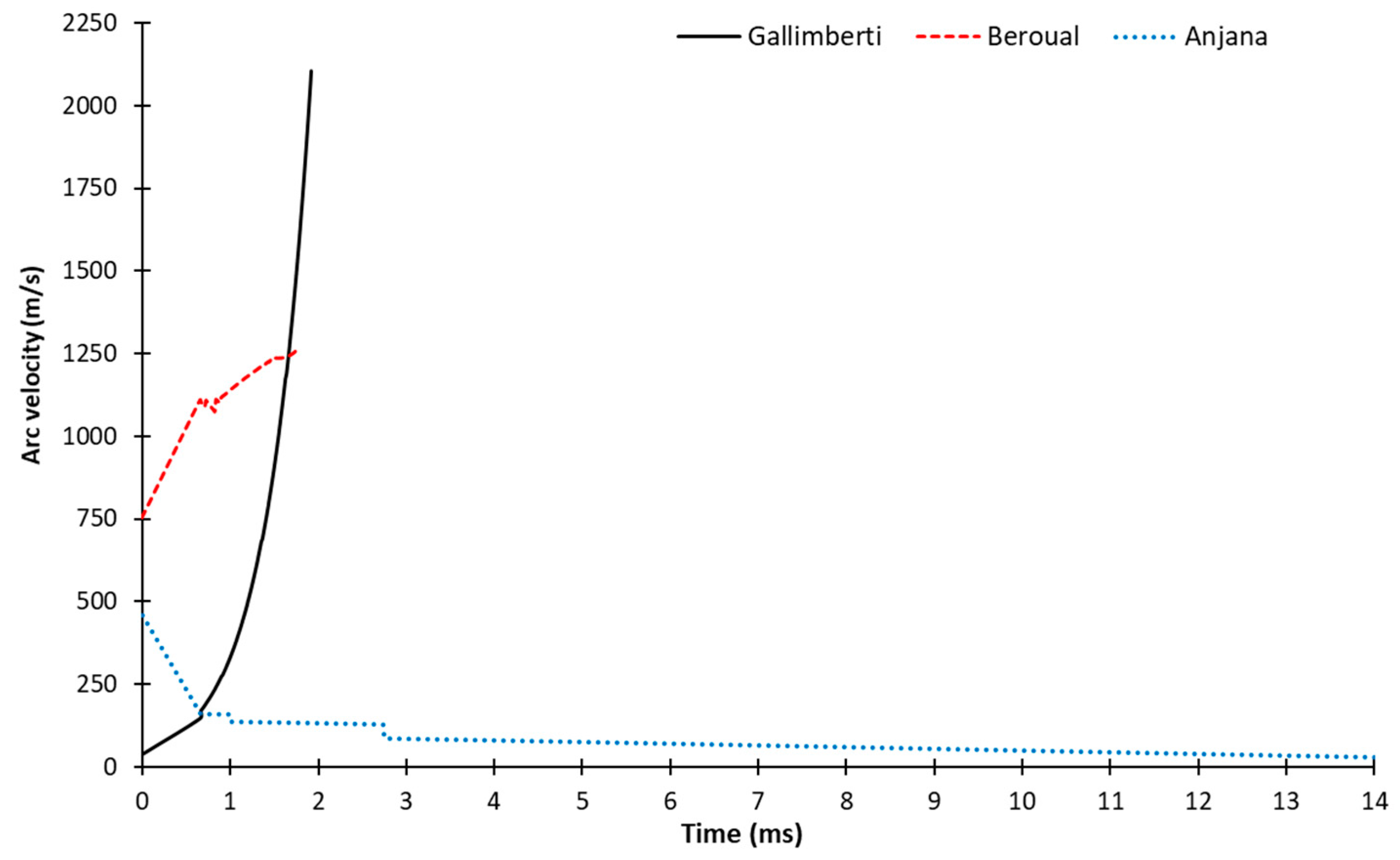
3. Study of the Influence of Arc Velocity Criteria

3.1. Arc Velocity Criteria

For this study, three different arc velocity criteria selected from the literature were implemented. These criteria were used in several mathematical predictive models dedicated to both polluted and ice-covered insulators and demonstrated good agreement with experimental results. Moreover, the chosen criteria use three different concepts to determine the arc velocity: arc current, power dissipated in the arc and arc mobility.

3.1.1. Gallimberti Criterion

The first criterion is the Gallimberti formulation (Equation (9)) used on in mathematical predictive models for polluted and ice-covered insulators. This formulation postulates that propagation velocity is proportional to arc current Im according to the following expression [39]:
v ( t ) = I m Q i ( t )
where Qi(t) is the required charge to induce arc propagation. This charge can be expressed as follows [39]:
Q i ( t ) = C i V a p
where Ci is the capacitance between the arc root and the ground and Vap the potential at the discharge head (arc root) given by Equation (7).
Capacitance Ci can be calculated using a spherical approximation [20] as follows:
C i = 4 π ε 0 r s i n h ( α ) i [ s i n h ( θ ) ] 1
with:
θ = c o s h 1 ( L x r )
where L is the insulator arcing distance, x the arc length and r the arc root radius given by Equation (5).

3.1.2. Beroual Criterion

The second criterion given by Equation (13), proposed by Beroual, was initially developed for discharges in dielectric liquids [40] and then successfully applied to model discharges in long air gaps as well as at the surface of polluted insulators [41] and more recently, on ice surfaces [18]. This criterion is based on the kinetic energy dissipated by the arc, which contributes to its propagation [40,41], and is expressed as follows:
ν ( t ) = 2 δ P ( t ) ρ π r 2 3
where v(t) is the arc velocity, δ is the required energy fraction for the discharge propagation, r is the arc root radius given by Equation (5), ρ is the air density and P(t) is the instantaneous power injected in the air-gap calculated numerically as follows:
P ( t ) = V m I m
where Vm is the source voltage given by Equation (1) and Im is the leakage current.
In order to take into account the presence of the ice layer, the parameter δ was fixed at 0.16 based on the results presented in [18]. This parameter is independent of the geometry and depends only on the environmental conditions related to arc propagation [18,19,41].

3.1.3. Anjan and Lakshminarassimh Criterion

Finally, the last criterion considered was proposed by Anjana and Lakshminarasimha (Equation (15)) where the arc velocity v is simply defined as the product of the arc mobility μ and the electric field Earc inside the arc [42]:
ν ( t ) = μ E a r c
where µ is the arc mobility (100 cm2/Vs) and Earc is the electric field along the arc given by Equation (2).

3.2. Experimental Set-Up and Simulation Parameters

In order to compare the influence of the different arc velocity criteria on the FOV results provided by the single-arc dynamic FEM model, several simulations were performed using the experimental results presented in [18]. These results were obtained from a simplified cylindrical physical model (Figure 4a) and a small post type ice-covered insulator (Figure 4b). For both physical models, ice was formed under wet-grown regime and a uniform ice deposit was obtained. Flashover tests were performed under melting conditions in order to obtain a uniform water film at the ice surface. AC FOV was determined using the up-and-down method recommended by the IEEE Standard 1783 and described in detail in [20]. The arcing distances used were 40, 80 and 103 cm respectively corresponding to three different freezing water conductivities, 30, 65 and 100 µS/cm. For the 40 and 80 cm arcing distances, the simplified insulator model was used (Figure 4a), whereas for the 103 cm arcing distance, a 119 cm long standard porcelain post type insulator was used (Figure 4b).
All parameters used for the single-arc dynamic FEM model were experimentally determined in previous studies [14,15,16,17] and are listed in Table 1. For all the simulations in this section were performed under the Hampton arc propagation criterion (Equation (4)) because of its facility of implementation in the calculation algorithm and also because it was used in our previous work on the single-arc FEM predictive model [33,34,35].

3.3. Influence of the Arc Velocity Criteria on the FOV Results

The AC FOV results obtained for each arc velocity criterion implemented in the calculation algorithm of Figure 3 were compared with experimental results from the literature, as presented in Table 2. Table 3 presents the relative absolute discrepancies obtained for each velocity criterion with these experimental results taken as reference.
In Figure 5 and Figure 6, leakage current for the three arc velocity criteria are compared as a function of time and arc length, respectively, for an arcing distance of 103 cm and a water conductivity of 100 µS/cm. Figure 7 presents the evolution of the same arc velocities as a function of time for the same simulation parameters.

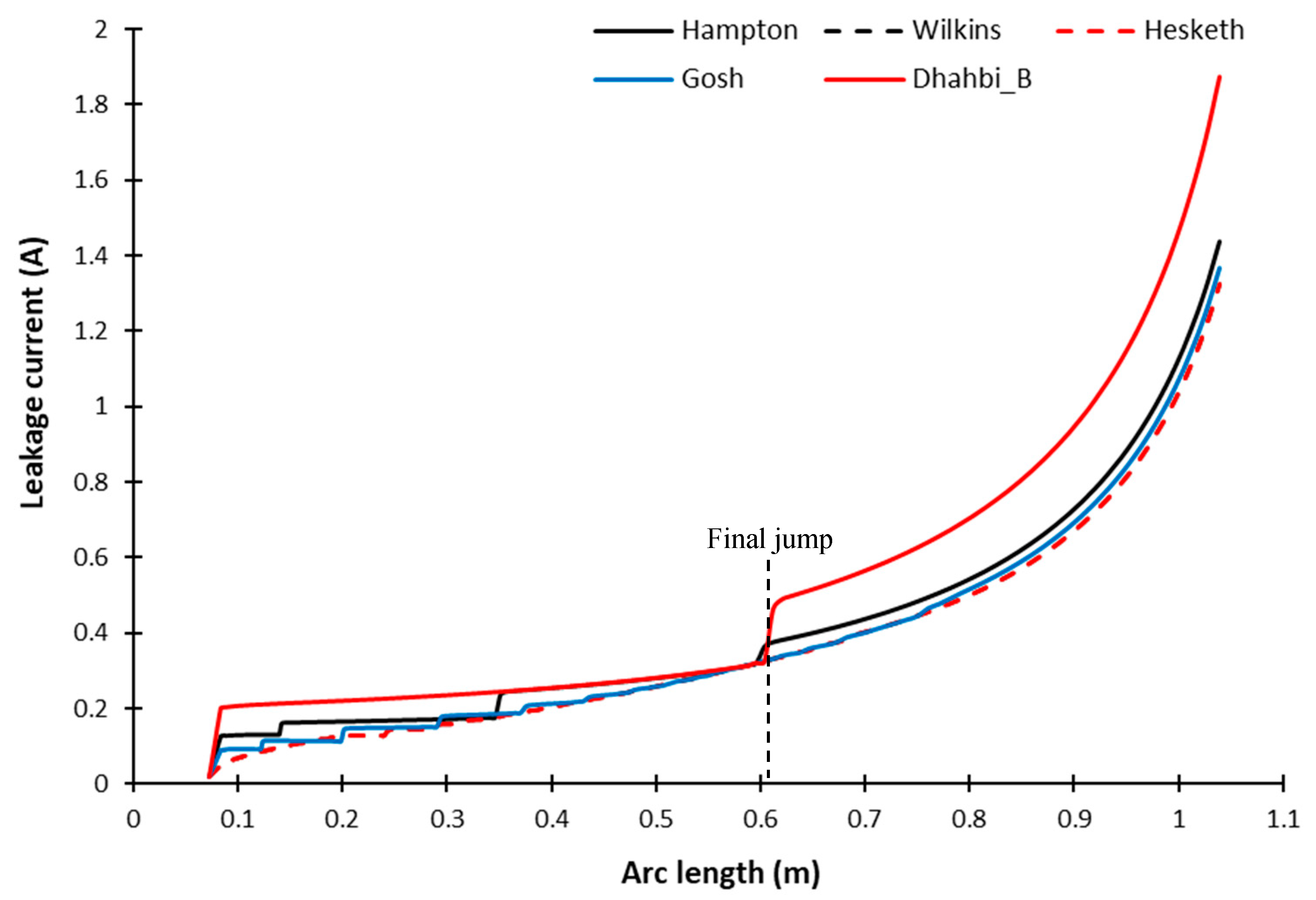
4. Study of the Influence of Arc Propagation Criteria

4.1. Arc Propagation Criteria

In this part, five propagation criteria were studied for the same arc velocity criterion, that of Gallimberti (Equation (9)). The Gallimberti criterion was chosen here as it yields the best accuracy in the predictive FOV results, as demonstrated in the previous section (see Table 3).

4.1.1. Hampton Criterion

Given by Equation (4), the Hampton criterion is based on the comparison between the E-field along the arc Earc (Equation (2)) and the average E-field Eavg inside the water film layer present at the ice surface. This criterion was used in our previous work as it is well adapted for FEM calculation and easier to implement [33,34,35].

4.1.2. Hesketh Criterion

Hesketh has argued that an arc in series with a conductive layer is self-adjusting in order to maintain a stable position. This means that the arc leaves its equilibrium position and propagates when the linear variation of the current in the arc channel is increasing. If the applied voltage is constant during the displacement of the arc, the propagation criterion is expressed by [43]:
d I m / d x > 0
where Im is the leakage current and dx is the elementary arc displacement.

4.1.3. Billings and Wilkins Criterion

Billings and Wilkins have supposed that the arc moves towards a new position allowing dissipation of maximum energy. This criterion is in fact a generalization of the criterion proposed by Hesketh (Equation (16)) but based on the power dissipated by the source voltage, which can be expressed as follows [44]:
d P ( t ) d x > 0
where dx is the elementary arc displacement and P(t) is the power injected by the voltage source given by Equation (14).

4.1.4. Gosh Criterion

Ghosh et al. have proposed a propagation criterion based on the assumption that the arc propagates when its resistance Rarc decreases comparatively to its elongation as follows [45]:
( d R a r c ) / d x < 0
where dx is the elementary arc displacement and Rarc is the arc resistance.
In order to implement the propagation criterion proposed by Ghosh et al. given by Equation (18), it was decided to use the expression of the arc resistance developed by Mayer, which can be expressed as follows [46]:
d d t [ l n 1 R a r c ] = 1 τ ( V a r c I m P 0 1 )
where τ = 100 µs is the temporal constant of the arc [36] and P0 the power dissipated in the arc, expressed numerically as
P 0 = E a r c x I m
where Im is the leakage current (A), x the arc length and Earc is the electric field along the arc given by Equation (2).
The development of Equation (19) for its implementation in the calculation algorithm presented on Figure 3 leads to the following expression:
d R a r c = [ ( R a r c τ ) ( 1 R a r c I m E a r c ) ] d t

4.1.5. Dhahbi and Beroual Criterion

The study of Dhahbi and Beroual established a new condition necessary for the propagation of the arc [47,48]. The proposed criterion indicates that if the resistance of the arc Rarc is lower than the residual resistance R(x), then the arc propagates. This condition is expressed in the following form:
R a r c < R ( x )
where Rarc is the arc resistance given by Equation (19) and R(x) is the residual resistance in series with the arc calculated by the FEM as follows:
R ( x ) = V a p / I m

4.2. Influence of the Arc Propagation Criteria on the FOV Results

Using the same procedure as the one used for the study on the influence of arc velocity criteria, each propagation criterion was implemented in the calculation algorithm presented on Figure 3 and the results obtained were compared with the same experimental results presented in the previous section using the simulation parameters of Table 1. The results for the AC FOV and the corresponding relative absolute discrepancy are presented in Table 4 and Table 5, respectively.
Figure 8 and Figure 9 compare the evolution of leakage current Im as a function of time and arc length respectively obtained for an arcing distance of 103 cm with a freezing water conductivity of 100 µS/cm. Figure 10 shows the corresponding arc velocity as a function of time.

5. Improvement of Gallimberti Arc Velocity Criterion

As demonstrated in Section 3.3., the arc velocity v(t) criterion proposed by Gallimberti has provided the more accurate results in terms of AC FOV prediction. As expressed by Equation (9), this criterion depends on the injected charge in the air gap Qi(t) (Equation (10)) by the arc, which also depends on the analytical calculation of the capacitance Ci between the arc root and the ground electrode using Equations (11) and (12).
As Ci is calculated using a spherical approximation used for simple geometries [19], it was decided to improve the accuracy of the Gallimberti criterion by numerically calculating Qi(t) using the FEM approach. For that purpose, an energetic approach was used based on Beroual’s studies on polluted insulator flashover, which leads to the formulation of his arc velocity criterion, given by Equation (13) [19]. From these studies, it was assumed that the kinetic energy required to propagate the arc represents a fraction of the total energy Wt dissipated in the conductive surface not bridged by the arc. This kinetic energy, Wp, can be expressed as follows:
W p = δ W t
with δ an experimental constant between 0.16 to 0.18 for an arc discharge propagating at the surface of a conductive layer [19].
Wp can then be linked to the injected charge Qi(t) used by Gallimberti (Equation (9)) as follows:
W p = 1 2 Q i ( t ) V a p
where Vap is the potential applied to the arc root.
The total energy Wt dissipated in the conductive surface not bridged by the arc can be easily obtained by FEM using the following equation:
W t = 1 2 V ε E 2 d V
where E is the electric field inside the conductive layer, ε the absolute permittivity of the water film and V the total volume of the conductive layer not bridged by the arc.
Once Wt is numerically determined using Equation (26), the velocity of the arc can now be calculated using Equations (9) and (25), leading to a new numerical formulation of the arc velocity expressed as follows:
v ( t ) = V a p I m 2 δ W t
All the parameters of this new arc velocity criterion were numerically determined using the numerical mono-arc model, except for the constant δ, which was fixed at 0.16 for the simulations.
The numerical arc velocity criterion was then implemented in the numerical mono-arc algorithm of Figure 3 and the results obtained were compared with those from the Gallimberti analytical velocity criterion used previously. The comparison of the results is presented in Table 6. Table 7 lists the corresponding discrepancies obtained for the two criteria compared to the experimental AC FOV values.
Figure 11 presents the comparison of the arc velocity obtained for the numerical and analytical criteria proposed by Gallimberti for an arcing distance of 103 cm with two freezing water conductivities: 30 µS/cm and 100 µS/cm. The initial arc length was fixed at 7% of the total arcing distance.

6. Discussion

6.1. Influence of the Arc Velocity Criteria

As a first observation, the results of Table 2 and Table 3 clearly demonstrate that the arc velocity criterion proposed by Gallimberti provides the best FOV predictive results with an average discrepancy of 4.7%. This value can be compared to the average discrepancy of 12.0% for the criterion of Beroual and 11.4% for Anjana and Lakshminarasimha. For the Gallimberti criterion, the accuracy of the FOV results obtained for each arcing distance is quite similar, at around 4.1%. However, this accuracy increases as the arcing distance is increasing for the Beroual criterion while it decreases for the Anjana criterion. In the case of Beroual, the decrease, from 18.5% at 40 cm to 3.4% at 103 cm, could be attributed to the fact that the proposed criterion was initially developed to simulate leader propagation in the long air gap, up to 16 m, with a different value of the energy fraction δ (see Equation (13)) [49]. In this case, the value of δ should be adapted to the length of the insulator in order to increase the accuracy of the results.
Hence, as a longer arcing distance provides longer arc length in the air, the Beroual criterion seems better adapted for longer insulators. The FOV accuracy decrease obtained for Anjana and Lakshminarasimha criterion, ranged from 6.8% at 40 cm to 14.5% at 103 cm. In this case, the proposed criterion seems better adapted for shorter arcing distance. These observations also permits to conclude that both Beroual and Anjana and Lakshminarasimha criteria seem to be influenced by the arcing distance, which is not the case for the Gallimberti criterion.
Concerning the results of Figure 5 and Figure 6, the leakage current Im values obtained with Gallimberti and Beroual are close, especially as a function of arc length (Figure 6), with similar leakage current values as well as similar the simulated time to flashover occurrence. The main difference between the two criteria can be observed from the arc velocity evolution as shown in Figure 7, where the Gallimberti trajectory seems more representative of the last stage of the flashover process, as concluded in several studies on polluted and ice-covered insulator flashover [5,18,20,47,48,49]. This last stage, also called final jump, is characterized by a slow increase in the leakage current and arc velocity until the arc length reaches its critical distance where a sudden increase of both current and arc velocity occurs, leading to flashover. With an arcing distance of 103 cm and freezing water conductivity of 100 µS/cm, the critical distance is around 62 cm (Figure 5) or 60% of the total arcing distance, which is consistent with the results reported in [17,18] and obtained with mathematical dynamic models.
However, these results are different from those obtained with the criterion of Anjana and Lakshminarasimha, which comes up with a leakage current value and a simulated time as high as seven time the value obtained for the other criteria. In the same time, the arc velocity evolution obtained with this criterion is not consistent with the flashover process where a decrease in the arc velocity is obtained when the leakage current increases. This particular evolution was reported in [48] for polluted insulators, which confirms the validity of our simulations. The arc velocity evolution obtained with Anjana and Lakshminarasimha can be attributed to the simplicity of the criterion and particularly to the value of the arc mobility taken as a constant along all the flashover process, as reported in [40,48].

6.2. Influence of the Arc Propagation Criteria

As first comment, the results obtained and presented in Table 4 and Table 5 seems to demonstrate that the criterion proposed by Billings and Wilkins seems to be the more accurate and the Hampton criterion the less one. However, the difference between the average discrepancies obtained for each criterion, ranging from 4.8% to 6.0%, is not so important in terms of FOV prediction. This confirms that the arc propagation criterion has less influence on the FOV predictive results that the arc velocity criterion. This also confirms that the Hampton criterion can be used as an arc propagation criterion [50], as this last one was initially proposed as a flashover criterion for short distance electrical arc by Hampton [36].
From the results presented on Figure 8, it can be observed that the leakage current evolutions obtained with the criteria proposed by, Billings and Wilkins, Gosh and Hesketh are very close. This can be principally explained by the similarity of their respective formulations, given by Equations (16) to (18), which are based on the same variation condition and are mainly dependent on leakage current Im, which is influenced by the simulation parameters and calculated by the numerical model. This is also confirmed by the results presented in Figure 9, where the leakage current charts as a function of arcing distance are very similar and where the critical distance is the same (equal to 60% of the insulator arcing distance). However, the Dhahbi and Beroual criterion seems to overestimate the final value of Im by 40% and the time to flashover by around 55% but not the final arc velocity value, as is observed in Figure 10. Also, for the Hampton criterion, the final value of Im is overestimated by only 8% and by 14% for the time to flashover.

6.3. Improvement of Gallimberti Arc Velocity Criterion

The results presented in Table 6 and Table 7 show that the implementation of the new arc velocity criterion increase substantially the accuracy of the FOV with an improvement of around 1.1% in the accuracy of the results compared to the Gallimberti analytical formulation. From the results of Figure 11, it can be observed that the evolution of arc velocity obtained with the modified criterion is different from the analytical formulation in terms of values. However, in terms of evolution, the modified criterion reproduces correctly the final jump reproducing the acceleration of the arc as approaching the ground electrode to finalize the flashover process. Moreover, the modified criterion also allows to take into account the effect of freezing water conductivity with a decrease of the time to flashover and an increase in the arc velocity as conductivity increases.

7. Conclusions

Thanks to the development of a generic calculation algorithm coupled to a commercial finite element software, it was possible to develop a new dynamic numerical mono-arc model to simulate the final stage of the flashover process of ice-covered insulators. Using the finite element method, it was possible to avoid the problem of analytical formulation for residual resistance calculation, which can only be applied to simple geometries. It was also possible to develop a generic algorithm that is independent of the different arc velocities and propagation criteria used. With the proposed generic model, it is now possible to study for the first time the effect of arc velocity and arc propagation criteria on FOV accuracy as well as on the evolution of leakage current and arc velocity.
The results obtained conclusively showed that the arc velocity criterion has a stronger influence of the FOV results when the same arc propagation criterion is used. The accuracy of the FOV results seems particularly affected by the presence of experimentally dependent constants as the energy fraction δ or arc mobility µ for the arc velocity criteria proposed by Beroual and Anjana and Lakshminarasimha. However, this is not the case with the arc velocity criterion proposed by Gallimberti, which provides more accurate FOV results. This criterion is a generic criterion as it depends on parameters, which can all be determined by the calculation algorithm without the need to be adjusted to different experimental conditions.
On the other hand, with the same arc velocity criterion based on the Gallimberti criterion, the FOV accuracy was found to be less affected by the arc propagation criterion with an accuracy variation between 4.8% and 6.0% for the five arc propagation criteria considered. This small variation in the FOV results can be attributed to the fact that all the arc propagation criteria studied presented no experimental dependent parameters as it was the case for some arc velocity criteria. Moreover, these results showed that the Hampton criterion, which was initially proposed as a flashover condition can also be used as an arc propagation criterion. Moreover, this criterion is well adapted for the proposed generic calculation algorithm based on electric-field calculation FEM software.
Finally, in order to propose a more generic mono-arc predictive model, it was decided to improve the Gallimberti arc velocity criterion by proposing a new numerical calculation of the capacitance Ci between the arc root and the ground electrode. This method, based on energetic considerations, was found to improve the accuracy of the FOV results by 1.1%. Moreover, as this improved Gallimberti criterion is totally determined numerically, there is no longer any restriction on its applicability to complex geometries, which is the aim of the generic mono-arc model proposed in this paper.

Author Contributions

Investigation, M.J.; Supervision, C.V. and I.F.

Funding

This research received no external funding.

Acknowledgments

The authors would like to thank the Natural Science and Engineering Research Council of Canada (NSERC), whose financial support made this research possible.

Conflicts of Interest

The authors declare no conflict of interest.

References

  1. Khalifa, M.M.; Morris, R.M. Performance of line insulators under rime ice. IEEE Trans. Power Appar. Syst. 1967, PAS-86, 692–698. [Google Scholar] [CrossRef]
  2. Meier, A.; Niggli, W.M. The influence of snow and ice deposits on supertension transmission line insulator strings with special reference to high altitude operation. In Proceedings of the IEEE Conference Publication 44, London, UK, September 1968; pp. 386–395. [Google Scholar]
  3. Kawai, M. AC flashover tests at project UHV on ice-coated insulators. IEEE Trans. Power Appar. Syst. 1970, 80, 1800–1804. [Google Scholar] [CrossRef]
  4. Farzaneh, M.; Chisholm, W.A. 50 Years of icing performance of outdoor insulators. IEEE Electr. Insul. Mag. 2014, 30, 14–24. [Google Scholar] [CrossRef]
  5. Farzaneh, M.; Chisholm, W.A. Insulators for Icing and Polluted Environments; John Wiley & Sons: Hoboken, NJ, USA, 2009. [Google Scholar]
  6. Fikke, S.M. Possible effects of contaminated ice on insulator strength. In Proceedings of the 5th International Workshop on Atmospheric Icing of Structures (IWAIS), Tokyo, Japan, 29 October–1 November 1990. [Google Scholar]
  7. Makkonen, H.; Komuro, H.; Takasu, K. Withstand voltage characteristics of insulator string covered with snow and ice. IEEE Trans. Power Deliv. 1991, 6, 1243–1250. [Google Scholar]
  8. Farzaneh, M.; Kiernicki, J. Flashover problems caused by ice build-up on insulators. IEEE Electr. Insul. Mag. 1995, 11, 5–17. [Google Scholar] [CrossRef]
  9. Chisholm, W.; Kuffel, J. Performance of insulation coating under contamination and icing conditions. In Proceedings of the CEA Spring Meeting, Vancouver, BC, Canada, 2–4 June 1995. [Google Scholar]
  10. Farzaneh, M.; Drapeau, J.F. AC flashover performance of insulators covered with artificial ice. IEEE Trans. Power Deliv. 1995, 10, 1038–1051. [Google Scholar] [CrossRef]
  11. Farzaneh, M. Ice accretion on high voltage conductors and insulators and related phenomena. Philos. Trans. R. Soc. A 2000, 358, 2971–3005. [Google Scholar] [CrossRef]
  12. Volat, C.; Farzaneh, M. 3-D modeling of potential and electric field distributions along an EHV ceramic post insulator covered with ice—Part I: Simulations during a melting period. IEEE Trans. Power Deliv. 2005, 20, 2006–2013. [Google Scholar] [CrossRef]
  13. Volat, C.; Farzaneh, M. 3-D modeling of potential and electric field distributions along an EHV ceramic post insulator covered with ice—Part II: Influence of air gaps and partial arcs. IEEE Trans. Power Deliv. 2005, 20, 2014–2021. [Google Scholar] [CrossRef]
  14. Farzaneh, M.; Zhang, J.; Chen, X. Modeling of the AC arc discharge on ice surfaces. IEEE Trans. Power Deliv. 1997, 12, 325–338. [Google Scholar] [CrossRef]
  15. Farzaneh, M.; Zhang, J. Modeling of DC arc discharge on ice surfaces. IEE Proc. Gener. Trans. Distrib. 2000, 147, 86–94. [Google Scholar] [CrossRef]
  16. Farzaneh, M.; Zhang, J. A multi-arc model for predicting AC critical flashover voltage of ice-covered insulators. IEEE Trans. Dielectr. Electr. Insul. 2007, 14, 1401–1409. [Google Scholar] [CrossRef]
  17. Farzaneh, M.; Fofana, I.; Tavakoli, C.; Chen, X. Dynamic modeling of DC arc discharge on ice surfaces. IEEE Trans. Dielectr. Electr. Insul. 2003, 10, 463–474. [Google Scholar] [CrossRef]
  18. Tavakoli, C.; Farzaneh, M.; Fofana, I.; Beroual, A. Dynamics and modeling of AC arc on ice surfaces. IEEE Trans. Dielectr. Electr. Insul. 2006, 13, 1278–1285. [Google Scholar] [CrossRef]
  19. Taheri, S.; Farzaneh, M.; Fofana, I. Improved dynamic model of DC arc discharge on ice-covered post insulator surfaces. IEEE Trans. Dielectr. Electr. Insul. 2014, 21, 729–739. [Google Scholar] [CrossRef]
  20. Taheri, S.; Farzaneh, M.; Fofana, I. Dynamic modeling of AC multiple arcs of EHV post station insulators covered with ice. IEEE Trans. Dielectr. Electr. Insul. 2015, 22, 2214–2223. [Google Scholar] [CrossRef]
  21. Mercure, H.P.; Drouet, M.G. Dynamic measurement of the current distribution in the foot of an arc propagating along the surface of an electrolyte. IEEE Trans. Power Appl. Syst. 1982, 101, 725–736. [Google Scholar] [CrossRef]
  22. Farokhi, S.; Nekahi, A.; Farzaneh, M. Mechanisms and processes of arc propagation over an ice-covered surface. IEEE Trans. Dielectr. Electr. Insul. 2014, 21, 2634–2641. [Google Scholar] [CrossRef]
  23. Nasser, E. Contamination flashover of outdoor insulation. ETZ-A 1982, 93, 321–325. [Google Scholar]
  24. Rahal, E.H.A.M. Sur les Mécanismes Physiques du Contournement des Isolateurs Haute Tension. Ph.D. Thesis, University Paul Sabatier, Toulouse, France, 1979. [Google Scholar]
  25. Jolly, D.C. Physical Process in the Flashover of Insulators with Contamination Surfaces. Ph.D. Thesis, Massachusetts Institute of Technology, Cambridge, MA, USA, 1971. [Google Scholar]
  26. Wilkins, R. Flashover voltage of high-voltage insulators with uniform surface-pollution films. Proc. Inst. Electr. Eng. 1969, 116, 457–465. [Google Scholar] [CrossRef]
  27. Flazi, F. Étude du Contournement Électrique des Isolateurs HT Pollués. Critères D’élongation de la Décharge Dynamique du Phénomène. Ph.D. Thesis, Université Paul Sabatier, Toulouse, France, 1987. (In French). [Google Scholar]
  28. Slama, M.E.-A. Étude Expérimentale et Modélisation de L’influence de la Constitution Chimique et de la Répartition de la Pollution Sur le Contournement des Isolateurs HT. Ph.D. Thesis, École Centrale de Lyon, Lyon, France, 2011. (In French). [Google Scholar]
  29. Water, R.T.; Haddah, A.; Griffiths, H.; Harid, N.; Sarkar, P. Partial arc and spark models of the flashover of lightly polluted insulators. IEEE Trans. Dielectr. Electr. Insul. 2010, 17, 417–424. [Google Scholar] [CrossRef]
  30. Rizk, F.A.M.; Rezazada, A.Q. Modeling of altitude effects on AC flashover of polluted HV insulators. IEEE Trans. Power Deliv. 1997, 12, 810–822. [Google Scholar] [CrossRef]
  31. Matsumoto, T.; Ishi, M.; Kawamura, T. Optoelectronic measurement of partial arcs on contaminated surface. IEEE Trans. Electr. Insul. 1984, 19, 531–548. [Google Scholar] [CrossRef]
  32. Hadi, H. Mécanismes de Contournement et sa Modélisation Dynamique Appliquée Aux Isolateurs Réels. Ph.D. Thesis, Université des Sciences et Technologies d’Oran, Bir El Djir, Algeria, 2002. (In French). [Google Scholar]
  33. Volat, C.; Farzaneh, M.; Mhaguen, N. Improved FEM models of one-and two- arcs to predict AC critical flashover voltage of ice covered insulators. IEEE Trans. Dielectr. Electr. Insul. 2011, 18, 393–400. [Google Scholar] [CrossRef]
  34. Jabbari, M.; Volat, C.; Farzaneh, M. A new single-arc AC dynamic fem model of arc propagation on ice surfaces. In Proceedings of the IEEE Electrical Insulation Conference (EIC), Ottawa, ON, Canada, 3–7 June 2013; pp. 360–364. [Google Scholar]
  35. Jabbari, M.; Volat, C.; Fofana, I. Application of a new dynamic numerical model to predict polluted insulator flashover voltage. In Proceedings of the IEEE Electrical Insulation Conference (EIC), Philadephia, PA, USA, 8–11 June 2014; pp. 102–106. [Google Scholar]
  36. Hampton, B.F. Flashover mechanism of polluted insulation. Inst. Electr. Eng. IEE 1964, 111, 985–990. [Google Scholar] [CrossRef]
  37. Rumeli, A. Computation of Pollution Flashover Voltages of High Voltage Insulators; Technical Report; Tubitak Engineering Research Group: Ankara, Turkey, 1973. [Google Scholar]
  38. Bessedik, S.A.; Hadi, H.; Volat, C.; Jabbari, M. refinement of residual resistance calculation dedicated to polluted insulator flashover models. IEEE Trans. Dielectr. Electr. Insul. 2014, 21, 1207–1215. [Google Scholar] [CrossRef]
  39. Bondiou-Clergerie, A.; Gallimberti, I. Theoretical modelling of the development of the positive spark in long gaps. J. Phys. D. Appl. Phys. 1994, 27, 1252–1266. [Google Scholar] [CrossRef]
  40. Beroual, A. Electronic gaseous process in the breakdown phenomena of dielectric liquids. J. Appl. Phys. 1993, 73, 4528–4533. [Google Scholar] [CrossRef]
  41. Beroual, A.; Dhahbi-Megriche, N. Model for calculation of flashover characteristics on polluted insulating surfaces under DC stress. In Proceedings of the 1998 Annual Report Conference on Electrical Insulation and Dielectric Phenomena (Cat. No.98CH36257), Atlanta, GA, USA, 25–28 October 1998; pp. 80–83. [Google Scholar]
  42. Anjana, S.; Lakshminarasmha, C.S. Computed of flashover voltages of polluted insulators using dynamic arc model. In Proceedings of the 6th International Symposium on High Voltage Engineering, New Orleans, LA, USA, 28 August–1 September 1989. [Google Scholar]
  43. Hesketh, S. General criterion for the prediction of pollution flashover. Proc. Inst. Electr. Eng. 1967, 114, 531–540. [Google Scholar] [CrossRef]
  44. Billings, M.J.; Wilkins, R. Considerations of the suppression of insulator flashover by resistive surface films. Proc. Inst. Electr. Eng. 1966, 113, 1649–1653. [Google Scholar] [CrossRef]
  45. Ghosh, P.S.; Chatterjee, N. Polluted insulator flashover model. IEEE Trans. Dielectr. Electr. Insul. 1995, 2, 128–136. [Google Scholar] [CrossRef]
  46. Mayr, O. Beitrag zur Theorie des statischen und des dynamischen Lichtbogens. Arch. Elektrotech. 1943, 37, 588–608. (In Germany) [Google Scholar] [CrossRef]
  47. Dhahbi-Megriche, N.; Beroual, A.; Krähenbühl, L. A new proposal model for flashover of polluted insulators. J. Phys. D. Appl. Phys. 1997, 30, 889–894. [Google Scholar] [CrossRef]
  48. Dhahbi-Megriche, N.; Beroul, A. Flashover Dynamic Model of Polluted Insulators under AC Voltage. IEEE Trans. Electr. Insul. 2000, 7, 283–289. [Google Scholar] [CrossRef]
  49. Fofana, I.; Beroual, A. A new proposal for calculation of the leader velocity based on energy consideration. J. Phys. D Appl. Phys. 1996, 29, 691–696. [Google Scholar] [CrossRef]
  50. Sundararajan, R.; Sadhureddy, N.; Gorur, R. Computer-aided Design of Porcelain Insulators under Polluted Conditions. IEEE Trans. Dielectr. Electr. Insul. 1995, 2, 121–127. [Google Scholar] [CrossRef]
Figure 1. Single-arc model of flashover on ice-covered insulator.
Energies 11 02807 g001
Figure 2. Modelling of a uniform ice-covered post type insulator of diameter D and arcing distance length L: (a) ice accretion geometry with one air gap, (b) ice accretion modelling and (c) FEM ice accretion model with the arc root.
Energies 11 02807 g002
Figure 3. Flowchart of the calculation algorithm developed for the single-arc dynamic FEM model.
Energies 11 02807 g003
Figure 4. Physical models of ice-covered insulators [18]: (a) simplified cylindrical model with an arcing distance of 40 cm and 80 cm; (b) porcelain post type insulator with an arcing distance of 103 cm. Reprint with permission [18]; 2008, IEEE.
Energies 11 02807 g004
Figure 5. Comparison of leakage current Im as function of time obtained for different arc velocity criteria with an arcing distance of 103 cm and a freezing water conductivity of 100 µS/cm.
Energies 11 02807 g005
Figure 6. Comparison of leakage current Im as function of the arc length obtained for different arc velocity criteria with an arcing distance of 103 cm and a freezing water conductivity of 100 µS/cm.
Energies 11 02807 g006
Figure 7. Comparison of arc velocity v(t) as function of time obtained for different arc velocity criteria with an arcing distance of 103 cm and a freezing water conductivity of 100 µS/cm.
Energies 11 02807 g007
Figure 8. Comparison of the leakage current Im as function of time obtained for different arc propagation criteria with an arcing distance of 103 cm and a freezing water conductivity of 100 µS/cm.
Energies 11 02807 g008
Figure 9. Comparison of the leakage current Im as function of the arc length obtained for different arc propagation criteria with an arcing distance of 103 cm and a freezing water conductivity of 100 µS/cm.
Energies 11 02807 g009
Figure 10. Comparison of the arc velocity as function of time obtained for different arc propagation criteria with an arcing distance of 103 cm and a freezing water conductivity of 100 µS/cm.
Energies 11 02807 g010
Figure 11. Evolution of the arc velocity obtained for the numerical and analytical Gallimberti criteria for an arcing distance of 103 cm with two freezing water conductivities: 30 µS/cm and 100 µS/cm.
Energies 11 02807 g011
Table 1. Parameters used for single-arc dynamic FEM model.
ParametersValue
A204.7
n0.5607
k1118
b0.5277
α0.0675
β2.45
B0.875
Table 2. Comparison of AC FOV obtained with each arc velocity criterion.
Water Conductivity (µS/cm)Experimental FOV [18] (kVrms)FOV Obtained with Gallimberti
(kVrms)
FOV Obtained with Beroual
(kVrms)
FOV Obtained with Anjana and Lakshminarasimha (kVrms)
Arcing distance of 40 cm
304849.653.551.4
654342.450.649.1
1004037.550.641.8
Arcing distance of 80 cm
308692.390.791.7
657878.988.384.5
1007469.689.489.3
Arcing distance of 103 cm
30106112.6102.6123
659797.092.2101.8
1009286.594.1115.7
Table 3. Comparison of relative absolute discrepancy obtained with each arc velocity.
Water Conductivity (µS/cm)Gallimberti
(%)
Beroual
(%)
Anjana and Lakshminarasimha
(%)
Arcing distance of 40 cm
303.311.47.0
651.417.64.5
1006.226.59.0
Arcing distance of 80 cm
307.35.46.6
651.115.88.3
1005.020.820.6
Arcing distance of 103 cm
306.23.216.0
650.04.94.9
1006.02.225.7
Average discrepancy (%)4.112.011.4
Table 4. Comparison of AC FOV obtained as a function of arc propagation criterion.
Water Conductivity
(µS/cm)
Experimental (kVrms)Hampton (kVrms)Billings and Wilkins (kVrms)Hesketh (kVrms)Ghosh (kVrms)Dhahbi and Beroual (kVrms)
Arcing distance of 80 cm
308692.384.792.592.692.5
1007469.669.471.671.671.6
Arcing distance of 103 cm
30106112.6112.2112.4112.4112.4
1009286.586.5888888
Table 5. Comparison of relative absolute discrepancy obtained with each arc propagation criterion.
Water Conductivity
(µS/cm)
Hampton (%)Billings and Wilkins (%)Hesketh
(%)
Ghosh (%)Dhahbi and Beroual (%)
Arcing distance of 80 cm
307.31.57.67.77.6
1005.06.23.23.23.2
Arcing distance of 103 cm
306.26.25.86.06.0
1006.06.05.84.34.3
Average discrepancy (%)6.14.85.35.35.3
Table 6. Comparison of AC FOV obtained with the new numerical arc propagation criterion with the arc velocity criterion of Gallimberti.
Water Conductivity
(µS/cm)
Experimental FOV [8] (kVrms)FOV with Numerical Criterion
(kVrms)
FOV with Gallimberti Criterion
(kVrms)
Arcing distance of 40 cm
304850.149.6
654342.942.4
1004038.737.5
Arcing distance of 80 cm
308692.693.3
657879.878.9
1007471.668.6
Arcing distance of 103 cm
30106113.4114.8
659797.497.0
1009287.886.5
Table 7. Comparison of the relative absolute discrepancy obtained with the new numerical and Gallimberti arc propagation criteria.
Water Conductivity
(µS/cm)
Discrepancy Obtained with Numerical Criterion (%)Discrepancy Obtained with Gallimberti Criterion (%)
Arcing distance of 40 cm
304.33.3
650.21.3
1003.26.2
Arcing distance of 80 cm
307.68.4
652.31.5
1003.27.2
Arcing distance of 103 cm
306.98.3
650.40
1004.55.9
Average discrepancy (%)3.64.7

