Electric Vehicle Charging Scheduling by an Enhanced Artificial Bee Colony Algorithm †

Department of Computer Science, University of Oviedo, 33204 Gijón, Spain
*
Author to whom correspondence should be addressed.
†
This paper is an extended version of our paper published in: García-Álvarez, J.; González, M.; Vela, C.; Varela, R. Electric Vehicle Charging Scheduling Using an Artificial Bee Colony Algorithm. In Ferrández Vicente J., Álvarez-Sánchez J., de la Paz López F., Toledo Moreo J., Adeli H. (eds) Natural and Artificial Computation for Biomedicine and Neuroscience. IWINAC 2017. Lecture Notes in Computer Science, vol. 10337. pp. 115–124. Springer, Cham.
Energies 2018, 11(10), 2752; https://doi.org/10.3390/en11102752
Submission received: 11 September 2018
/
Revised: 3 October 2018
/
Accepted: 11 October 2018
/
Published: 14 October 2018
Abstract
:Scheduling the charging times of a large fleet of Electric Vehicles (EVs) may be a hard problem due to the physical structure and conditions of the charging station. In this paper, we tackle an EV’s charging scheduling problem derived from a charging station designed to be installed in community parking where each EV has its own parking lot. The main goals are to satisfy the user demands and at the same time to make the best use of the available power. To solve the problem, we propose an artificial bee colony (ABC) algorithm enhanced with local search and some mating strategies borrowed from genetic algorithms. The proposal is analyzed experimentally by simulation and compared with other methods previously proposed for the same problem. The results of the experimental study provided interesting insights about the problem and showed that the proposed algorithm is quite competitive with previous methods.

1. Introduction
Electric Vehicles (EVs) are increasingly important nowadays for environmental reasons. However, their sustainable deployment requires new technology and infrastructures as, for example, specialized charging stations to accommodate large fleets of EVs. There have been considerable research effort on different aspects related to EV charging as, for example, the location of EV charging stations [1,2,3,4] or electricity price forecasting [5], among others. Charging scheduling is particularly interesting due to the large charging times often required by batteries and also to the power and physical constraints of the charging stations. Only with the use of smart scheduling algorithms is it possible to make the best use of the available resources and to satisfy the user requirements at the same time [6,7].
In this paper, we tackle the problem raised in [8], which is motivated by a charging station designed to be exploited in a residential parking where each vehicle must be parked in its owner’s space. This physical constraint, together with others derived from the electric characteristics of the charging station, makes the problem of scheduling the EV’s charging times over periods of large demand difficult. For this reason, a number of metaheuristics were proposed to solve the problem, in particular dispatching rules [8], memetic algorithm [9] and artificial bee colony (ABC) algorithm [10].
In this paper, we build on the work presented in [10] and include a number of new contributions, in addition to a thorough updating of the literature review: (1) We introduce several new strategies for both employed and onlooker bee phases, which contribute to improving the performance of the ABC algorithm so that it is able to reach much better solutions; (2) We hybridize the algorithm with an additional local search step, which allows the algorithm to further improve the final solution; (3) We performed a much more comprehensive experimental study using a larger set of instances than that used in previous studies, in which we compare our proposals and show that the new hybrid algorithm was able to improve the quality of the results reported in [8,9,10].
The remainder of this paper is organized as follows: in Section 2, we review the literature on EV charging scheduling. In Section 3, we present the characteristics of the charging station considered herein. Section 4 defines the scheduling problem. In Section 5, we describe the artificial bee colony algorithm and the proposed enhancements. The results of the experimental study are reported and analyzed in Section 6. Finally, Section 7 summarizes the main contributions of this paper and proposes some ideas for further work.
2. Literature Review
EV charging raises challenging scheduling problems. Indeed, the research community has proposed a number of EV charging scheduling models in the last years. Some comprehensive reviews of such problems and solving techniques are given in [6,7,11].
There are two main strategies for scheduling EV charging. The first one is distributed or decentralized strategy [12,13,14], which offers great flexibility to EV owners, allowing them to decide about when and how to charge their EVs. This may give rise to some security problems and overload in the power grid. Some of these inconveniences may be avoided to some extent by imposing some price incentives that stimulate EV owners to charge their EVs in off-peak hours (see, for example, [15,16]). However, it is generally difficult to achieve an optimal charging strategy [17].
The second strategy is centralized charging, in which an aggregator makes all the scheduling decisions as starting time and charging rate of the EVs. In order to build a schedule, the aggregator receives the status of all EVs along with their desired departure times (provided by EV owners) and tries to optimize both the customers satisfaction and the use of the available power [18]. Most papers in the literature recommend this strategy over the decentralized one. Indeed, some studies demonstrate that a coordinated charging scheme with some valley-filling strategy significantly outperforms uncoordinated charging by suppressing elevated peak load demands on the power grid [19].
Regarding the objectives pursued, there are a number of strategies. Some papers perform single objective optimization of total cost [20,21], total tardiness [22] or the use of renewable energy sources [23]. It is also usual to minimize peak demands or grid congestion [17,24]. Other approaches consider three-phase power flows and try to minimize the imbalance between phases [8,25]. Clearly, in these types of problems, there may be many relevant objectives, and therefore multi-objective optimization is often considered. For example, in [26], the optimization of the total load variance and EV owners’ preferences is considered. Another interesting example can be found in [27], where the objectives are the minimization of the costs incurred from being parked, maximization of the revenues offering secondary regulation and the maximization of the vehicle fleet charging station efficiency.
It is important to mention that each environment and EV charging station present particular characteristics, so each of them gives rise to a different model and poses its own scheduling problem. For example, some systems consider varying the charging rate of the EVs [24], varying power of the charging station [28], or varying electricity prices [29,30]. Other models consider uncertainty and stochastic parameters [31,32]. Another issue is whether [33] or not [8] the scheduler can decide to which dock each EV is assigned. Some models even consider charging/discharging strategies to optimize the overall process [34].
Due to the complexity of these problems, many existing optimization techniques have been applied to solve them—for example, linear programming [35], ant-based swarm algorithm [12], genetic algorithm [27], particle swarm optimization [21,36], multi-agent based system [37], estimation of distribution algorithm [30], moving window optimization [29], tabu search and GRASP [38], among others.
As mentioned, the model considered in this work is that proposed in [8]. This model corresponds to the charging station described in [39], which is designed to be installed in community parking. In this station, a parking lot has a charging point connected to one of the lines of a three-phase feeder. This, together with the fact that each user must use his own parking lot, gives rise to the main constraint of the model: the load imbalance on the three lines must be limited. The solution proposed in [8] relies on the use of dispatching rules to meet online scheduling requirements. For this reason, the quality of the solutions is moderate and may be improved as demonstrated in further studies [22] by means of offline algorithms. Hence, two new approaches were proposed in order to obtain better solutions, memetic algorithm [9] and artificial bee colony algorithm [10]. We argue that the results of the later could still be improved with some intensification step. To this end, we propose incorporating problem domain knowledge by local search and some other improvements in different phases of the artificial bee colony algorithm.
3. The Charging Station
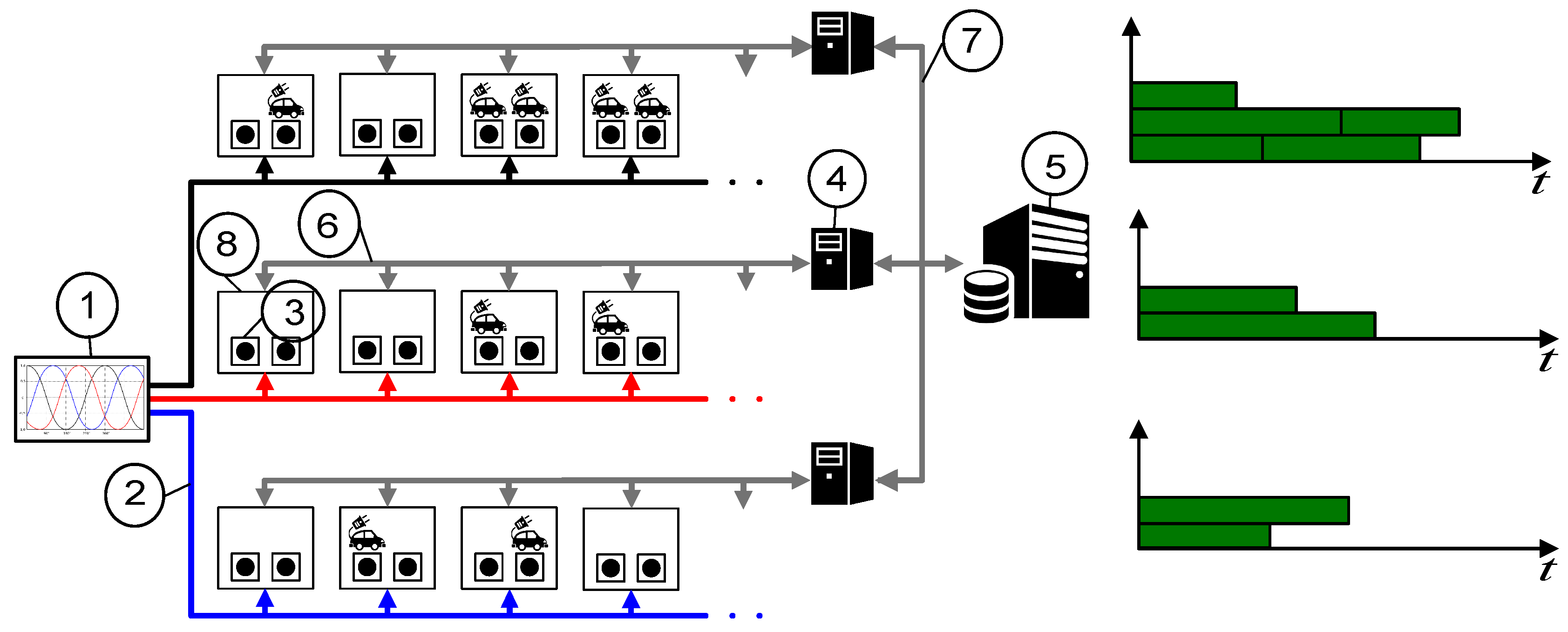
The design and operation modes of the charging station is detailed in [39]; Figure 1 shows its general structure. The station is fed by three-phase electric power with voltage between phases of 400 V. Each charging point is connected to one single-phase at 230 V and 7.3 kW (32 A). In principle, we follow a so-called Mode 3 in the regulation UNE-EN 61851-1 [40], which considers charging at a constant rate. As pointed in [41], this is the most suitable method for domestic environments.
As shown in Figure 1, the station is controlled by a server together with a number of masters and slaves. Each slave controls two charging points of type 2/AC IEC 62196-2. A master is connected to eight slaves and has a user interface. The server centralizes the control and receives signals from the slaves regarding events as connection or disconnection of EVs. The server also sends orders to the slaves to activate and deactivate charging points in accordance with the schedule.
Even though there are many spaces available (180 in our experimental study), not all the charging points in these spaces can be active at the same time due to the available power being limited. For example, if electricity supply of 50 kW three phase power (3/AC) were contracted and each EV requires 7.3 kW, at most 21 EVs can be charging simultaneously in a line at the maximum power. To avoid energy losses, the imbalance among the three lines must be limited. To this end, a hard maximum imbalance between every two lines is established.
4. Problem Definition
As it was done in [10], we consider the static and dynamic versions of the problem. The first one is not realistic, but it helps to better understand the problem and to establish performance limits to the solution to the dynamic problem, which models the real scenario. Finally, we comment on some model extensions.
4.1. The Static Problem
We have three lines with charging points each. Each line receives vehicles, denoted by . We denote by n the total number of vehicles, i.e., . For each vehicle, we are given the arrival time , the charging time and the due date , namely the time at which the user is expected to take the vehicle away. In this static version, it is assumed that all these data are known in advance at the beginning of the scheduling horizon ().
The objective is to build up a feasible schedule; i.e., to establish starting times , , , for charging the EVs so that the following constraints are satisfied:
where is the completion time of charge of the EV , n is a parameter that fixes the maximum number of EVs that can be charging in a line at the same time (due to the contracted electricity supply, as described in Section 3), is the number of EVs charging at the same time in the line i over the interval and is a parameter.
Equation (1) forbids EVs to start charging before their arrival time. Equation (2) ensures that EVs cannot be disconnected until they finish charging. Equation (3) establishes that the number of EVs charging in a line cannot exceed n . Finally, Equation (4) establishes the maximum imbalance between any two lines by means of the parameter .
The objective function is the total tardiness defined as:
which should be minimized.
4.2. The Dynamic Problem
In the dynamic problem, we do not know in advance the due dates, charging and arrival times of the vehicles. Therefore, following [8], it is modeled as a sequence of static instances at times . The instance is given by the EVs in the system arriving by that have not completed charging. Some of them have started to charge before and we know their completion times , while others have not yet started to charge. For these last ones, we know the charging times and due dates . The goal is to obtain a feasible schedule for these EVs that minimize the total tardiness and that satisfy all the constraints naturally derived from the static problem.
At each time point , a supervisor program running on the server checks for new EV arrivals since . If some EV arrived, a new instance is created and solved; otherwise, the current schedule remains valid until the next time point. Notice that the may be modified in further instances as long as does not start charging. The time interval is set at two minutes in order to not overload the server in situations where many EVs arrive at almost the same time and also to make the best use of the charging resources. For more detailed definition of the dynamic problem, we refer the interested reader to [8].
4.3. Model Extensions
In previous descriptions of the charging model, we have done some simplifying assumptions for the sake of clarity, namely, all EVs charge at the same constant rate, the user never takes the EV away before the completion time of charging, the batteries never get fully charged before this time, and the contracted power in the charging station is constant over time. However, the model may be extended to deal with these situations as well. For example, variable contracted power may be modeled by considering that the capacity of each line is organized into slots whose number varies over time. Therefore, charging at a variable rate is possible by assigning an EV a different number of slots at different time intervals. In addition, situations such as EVs going out or EVs completing charging before their charging times may be managed by events that the slaves can identify and communicate to the server, much in the same way as when a new EV arrives. With all of these, the energy requirement of an EV should be given as the number of time slots required to reach the desired state of charge of the battery. Of course, with these extensions, the scheduling problem will be harder to solve, but the proposed algorithms could be naturally adapted.
5. Artificial Bee Colony Algorithm
The Artificial Bee Colony algorithm (ABC) is a swarm population-based metaheuristic introduced in [42], which is inspired by the intelligent foraging behavior of honey bees. The method mimics the search for food of three types of foraging bees: employed, onlooker and scout. ABC is often used to solve scheduling problems because of its effectiveness and its good balance between diversification and intensification. A review of its fundamentals and some applications can be found in [43]. The ABC algorithm was proposed for numerical optimization and so, in principle, the food sources should be encoded by vectors of real numbers in a given interval. However, unlike other similar metaheuristics as Particle Swarm Optimization (PSO), whose variation operators strongly rely on accurate distance metrics between solutions, ABC is easy to adapt to discrete; i.e., combinatorial, optimization. This was done, for example, in [44] where the authors tackled a variant of the Flow Shop Scheduling problem and encode food sources by permutations of jobs. We use similar coding schema for the EV charging scheduling problem herein.
As shown in Algorithm 1, the proposed ABC algorithm starts creating a number of initial solutions or food sources. Then, it iterates over a number of cycles. In each cycle, several steps are performed: employed bee phase, onlooker bee phase and scout bee phase. The termination criterion is satisfied when the best solution is not improved for a consecutive number of cycles, or if a solution with zero tardiness is reached. Finally, local search is applied to the best solution found so far. The main features and steps of this algorithm are described below.
| Algorithm 1 The Artificial Bee Colony algorithm |
Input An EV charging scheduling problem instance P
|
5.1. Food Source Representation and Evaluation
We encode solutions; i.e., food sources, as permutations of EVs. In the static problem, all EVs of the problem are considered as the algorithm is applied only once to solve the problem. However, in the dynamic problem, the algorithm is applied to solve each instance and so the permutation contains only the EVs at that do not start to charge. Each solution has an associated value, , which is the number of times it was tried to improve without success.
To evaluate a food source, a schedule S is built from the permutation by sequentially scheduling the EVs at the earliest possible starting time such that all the constraints defined in Section 4 are met with respect to the EVs previously scheduled. The amount of nectar (the measure of quality of a solution) is the value , where is the tardiness of the solution calculated by Equation (5). Abusing the language, in the following, we will use the symbol S to denote both the schedule and the permutation of EVs corresponding to a given solution.
5.2. Initial Population
We propose combining two dispatching rules with some random food sources to create an initial population. The goal is to achieve good balance among quality and diversity. The first dispatching rule is the Due Date Rule (DDR), which sorts all vehicles in increasing order of their due dates . The second is the Latest Starting Time (LST) rule, which sorts all vehicles in increasing order of their latest starting times, defined as . Both rules are deterministic, so we follow the approach proposed in [22] to create diverse food sources. To add the next vehicle to the permutation V, we sort the vehicles not yet added to V using the corresponding dispatching rule and then we perform a tournament selection: a number of vehicles is selected uniformly and the best of them according to the ordering given by the dispatching rule is added to V. As we will see, the parameter is actually relevant: too large values generate too similar food sources, whereas too small values generate almost random ones. To build up the initial population, one third of the individuals are generated by each dispatching rule and the other third at random.
5.3. Employed Bee Phase
Employed bees are in charge of searching for new and hopefully better food sources. To this end, in the original ABC algorithm, each employed bee generates one new candidate solution in the neighborhood of the solution in one food source. The new candidate replaces the old solution if it is better. In our algorithm, we propose exploiting crossover operators borrowed from genetic algorithms following two different approaches.
In the first one (denoted ), the best solution found so far is selected, unless it was already selected in previous cycles. In that case, we choose the food source with the largest such that it was never chosen for this role. This requires maintaining the list “common parents” containing the solutions that were already chosen. Then, the food source in each employed bee is combined with the selected food source, generating two new offspring. The best of them replaces the food source in the memory of the employed bee if it is better; in that case, is set to zero for this food source; otherwise, the original food source remains in the population with increased in one unit. The rationale of this method is that it may produce good solutions as a solution that was not improved after many trials may be a good solution. At the same time, it may produce reasonable diversity, as new solutions are always created from different outstanding food sources in successive cycles of the algorithm.
In the second approach (denoted ), we randomly shuffle the food sources of the population and organize them in pairs to be combined. Thus, all food sources in the population are combined. In this way, the diversity is expected to be larger than in the first method at the cost of lower quality.
We consider different crossover operators to combine solutions. The first one, which is specially designed for this problem, is the Starting-time Based Crossover (SBX), initially proposed in [22]. It randomly selects a time (where is the minimum starting time of all vehicles in both parents and is the maximum starting time), and builds the first offspring with all the EVs in the first parent that are scheduled before , in the order they appear in , followed by the remaining EVs in the same order as they appear in . The second offspring is created similarly by exchanging the roles of and . The second operator is the classic Partially-Mapped Crossover (PMX) proposed in [45], which is commonly used in permutations encoding. In addition, we consider a third option that consists of choosing SBX or PMX at random each time. In [10], it was proven that this method obtains better results than using each operator separately. In Section 6, we report results from some experiments carried out to compare all these options.
5.4. Onlooker Bee Phase
Employed bees share their information with onlooker bees waiting in the hive. Then, onlooker bees probabilistically choose their food sources to go. Once there, they try to find a better neighboring source. In particular, the probability to choose a food source k in this phase is
Notice that, in this case, divisions by zero will not be produced as the algorithm ends as soon as a solution with zero tardiness is reached.
We propose different ways to apply the onlooker bee phase, which are adapted to the EV charging scheduling problem. The rationale is trying to schedule a vehicle with tardiness earlier or to delay a vehicle without tardiness.
The first one, termed , is a generalization of the procedure proposed in [10], which selects at random up to the of the EVs in the permutation . For each selected EV, , its tardiness is checked. If it is zero, could possibly be delayed; therefore we try to swap with all the EVs from its position onwards, until an improving solution is found. However, if the tardiness is positive is swapped with the previous ones instead. In any case, as soon as an improving solution is reached, it replaces the original one and is set to zero. Otherwise, the original solution remains and is increased in one unit.
In this paper, we enhance this procedure by using two parameters: and . As soon as we find a swap that leads to a better solution, we set , and we repeat the process from this new solution, unless we have reached the maximum of improvements. On the other hand, is used so that not all swaps are tried, but only a swap for every vehicles. This new proposal may be better than that in [10] because the parameter allows for increasing the intensification (of course at the cost of increasing the computational time), whereas the parameter allows the algorithm to reduce the computational time, as it avoids testing all candidate swaps. The enhanced procedure is denoted and it is showed in Algorithm 2. The proposal described in [10] would be a particular case taking and .
| Algorithm 2 First type improvement for the onlooker bee phase |
| Input A solution S and parameters and |
| ; |
| ; |
| while and do |
| Select one vehicle randomly; |
| ; |
| if tardiness of then |
| ; |
| else |
| ; |
| end if |
| while and and do |
| Swap and in S to obtain ; |
| if is better than S then |
| ; |
| ; |
| end if |
| if tardiness of then |
| ; |
| else |
| ; |
| end if |
| end while |
| ; |
| end while |
| return The current solution S; |
The second way to apply the onlooker bee phase (denoted ) chooses EVs to move earlier or to delay depending on the structure of the schedule. Firstly, it considers whether to schedule tardy EVs earlier or to delay EVs without tardiness. This selection is done with probability proportional to the number of tardy EVs. For example, if 20% of EVs have zero tardiness, then we have 80% probability of trying to delay non tardy EVs and only 20% of trying to schedule tardy EVs earlier. The rationale behind this strategy is that when there are many tardy EVs, delaying some non tardy EV gives the chance for a large number of tardy EVs get scheduled earlier—while in situations with a small portion of tardy EVs, it is better trying to schedule earlier one of them each time. Furthermore, an additional control parameter determines the maximum number of swaps that we try for each single EV, so that it helps with further reducing the computational time. The detailed procedure can be seen in Algorithm 3.
5.5. Scout Bee Phase
When a solution cannot be improved after trials, its food source is abandoned and a scout bee is in charge of looking for a new source. To implement the scout phase, we replace all solutions having by random ones, and set for each of them.
| Algorithm 3 Second type improvement for the onlooker bee phase |
| Input A solution S and parameters , and |
| ; |
| random number in [0..1]; |
| ; |
| ; |
| while and do |
| if then |
| Select uniformly one non tardy EV ; |
| ; |
| else |
| Select uniformly one tardy EV ; |
| ; |
| end if |
| ; |
| ; |
| while and and and do |
| Swap and in S to obtain ; |
| ; |
| if is better than S then |
| ; |
| ; |
| ; |
| end if |
| if then |
| ; |
| else |
| ; |
| end if |
| end while |
| ; |
| end while |
| return The current solution S; |
5.6. Local Search
It is well known that hybridization with local search usually improves the results of an evolutionary metaheuristic, providing extra intensification [46,47,48]. Here, we propose applying a hill climbing procedure to the final solution reached by a ABC algorithm in the following way: we iterate over the EVs in the order they are scheduled and if the EV in position i () is tardy, we try to schedule it earlier, just before each one of the previous EVs in the schedule, where is a parameter. If an improving solution is reached, it substitutes the previous one and the iterative process is started again. The local search finishes when no improving solution is reached in a whole iterative process. The parameter is given a small value for the sake of efficiency and to introduce reasonably small changes in the neighboring solutions. Notice that the number of EVs for which is swapped depending on the position i; the rationale is that the chances of a EV being scheduled earlier in an improving schedule is in direct ratio with the position in the schedule. Algorithm 4 shows the detailed steps. In Section 6, we will see that this additional local search improves the results of the algorithm, and the extra computational time taken is small due to the fact that it is only applied to the best solution returned by the ABC algorithm.
| Algorithm 4 The local search |
| Input A solution S and the parameter |
| improvement ← True; |
| while improvement do |
| improvement ← False; |
| ; |
| while do |
| if tardiness of then |
| ; |
| ; |
| local_improvement ← False; |
| while local_improvement do |
| Swap and in S to obtain ; |
| if is better than S then |
| ; |
| improvement ← True; |
| local_improvement ← True; |
| end if |
| ; |
| end while |
| end if |
| ; |
| end while |
| end while |
| return The current solution S; |
6. Results
We have considered the benchmark proposed in [8] (publicly available in [49]), which consists of 2160 instances organized in 72 sets of 30 instances each. This benchmark is inspired in a prototype charging station with 180 spaces. The profiles of arrival times, demands and due dates correspond to the expected behavior of real users under different circumstances. The time horizon is one day and three different scenarios were considered: scenario 1 represents a normal week day, where vehicles arrive throughout the day, with two arrival peaks. Scenarios 2 and 3 represent more complex situations where the arrival time of most of the vehicles is at almost the same time. Scenario 3 having tighter due dates than scenario 2. Each set is characterized by the tuple ; has two possible values 1 and 2, in type 1 instances, one third of the vehicles arrive to each line, whereas in instances of type 2 the loads are unbalanced so that 60% of the vehicles arrive to line 1, 30% to line 2 and 10% to line 3. This unbalance among the lines makes type 2 instances harder to solve due to the difficulty in maintaining the constraint of maximum imbalance. Three values are considered for n, 20, 30 and 40, and four values for , 0.2, 0.4, 0.6 and 0.8.
The proposed algorithm is implemented in C++ programming language using a single thread, and the target machine is Xeon E5520 running Scientific Linux 6.0. Due to the stochastic nature of the ABC algorithm, 30 independent executions were done for each instance to obtain statistically significant results.
For the purpose of comparison, the main reference is the EVS algorithm proposed in [8]. After EVS, some new approaches were proposed, namely a Memetic Algorithm (MA) [9] and an Artificial Bee Colony (ABC) [10], which were able to improve the quality of the solutions from EVS at the cost of taking more execution time. Here, it is important to remark that there are prototype implementations of the charging station, but there are no actual implementations in a real parking yet, and so all previous experimental results considered were obtained by simulations.
To set up the best values of the parameters of the algorithm, we have conducted some experiments using a set of 24 instances, namely the first instance of each group of scenario 1. For all experiments, the stopping condition was adjusted so that the computational time of the different configurations was similar and comparable to that of other state-of-the-art algorithms. Table 1 summarizes the values tested for each parameter and the best values of the parameters for the static and dynamic versions of the problem.
Using the proposed parameter setting, which is shown in the columns “best static” and “best dynamic” of Table 1, and considering 25 consecutive iterations without improving the best solution obtained so far as stopping condition, we see that the convergence pattern is appropriate. As an example, Figure 2 shows the evolution of the total tardiness in a run of one scenario 1, type 1 instance with and , considering the static version of the problem.
From the results in Table 1, we may draw some interesting conclusions. For example, the second improvement proposed for the employed bee phase () performed better than the method proposed in [10]. Perhaps this is due to a larger diversity on the generated offspring. In addition, the best configuration for the onlooker bee phase ( with and higher than one) performs better than that proposed in [10] (which uses and ). It is also worth to mentioning that the final local search step is able to improve the final results of the ABC algorithm when using similar computational times in the comparison.
Using the best configuration reported in Table 1, we have performed experiments across the full benchmark with 2160 instances. Table 2, Table 3 and Table 4 report the results in scenarios 1, 2 and 3, respectively. For scenario 1, we report the results obtained by MA [9], ABC [10] and hABC. For the EVS algorithm [8], we only report tardiness values obtained for the dynamic problem, as that paper does not tackle the static one. For scenarios 2 and 3, we only show tardiness values from hABC along with those reported for EVS [8] and MA [9] on the dynamic problem. As in [10], there are no results reported from ABC on these scenarios. Each value in the Tables represents the sum of the tardiness (in hours) of the 30 instances of each group. The numbers in bold indicate that the best value for each version of the problem.
As it can be expected, the results reported in Table 2, Table 3 and Table 4 show that the tardiness values strongly depend on the problem characteristics , , n, . Instances with lower n and values present larger tardiness, which seems reasonable as these instances are much more constrained. Type 2 instances have larger tardiness than those of type 1 because of the bottleneck caused by the unequal distribution of EVs in the three lines. In addition, instances of scenario 1 have the lowest tardiness due to the EVs’ arrival being evenly distributed along the day, which allows for scheduling many EVs without tardiness. In addition, the tardiness obtained in static problems are generally much lower than those obtained in dynamic ones, which suggests that knowing in advance all the information allows the algorithms to obtain better schedules and that there may still be room to improve the solutions of the dynamic problem.
From Table 2, Table 3 and Table 4, it is also clear that ABC outperforms ABC [10] and EVS [8] in all groups of 30 instances with the same values of parameters n and , in both the static and dynamic versions of the problem. hABC also outperforms MA [9] in most cases, although the differences in the static problem considering scenario 1 are small. In order to assess that the improvement is statistically significant, following [50], we have performed non-parametric statistical tests for cases where we have multiple-problem analysis. First of all, a Shapiro–Wilk test confirmed the non-normality of the data. Then, we used paired Wilcoxon signed rank tests to compare the average results in all instances. In both the static and dynamic versions of the problem, we have obtained p-values lower than 2.2 × 10⁻¹⁶ against the other three state-of-the-art approaches. These tiny p-values confirm that the improvements in these instances are statistically significant, and so we can tell that hABC performs better than the other methods. If we perform a more detailed analysis, we find that specifically in type 2 instances from scenario 1 in the static version, the difference in the results obtained by hABC and MA is not statistically significant (the p-value when assessing if hABC is better than MA is 0.5735, and it is 0.8531 the other way around). In all other cases, hABC is always significantly better.
In order to visualize the structure of the schedules and to appreciate how the difficulty of the problems strongly depend on the different loads of the three lines, we show two complete schedules (types 1 and 2 respectively, and in both cases) for the dynamic problem in Figure 3 and Figure 4 (more schedulesare included in the complementary material of the paper). The schedule in Figure 3 shows a normal situation where the load is balanced in the three lines so that all EVs are scheduled almost without tardiness and at the same time the maximum imbalance () is only reached over small periods of time. However, the schedule in Figure 4 represents an extreme situation (which probably will not happen in the real environment) where EVs are unevenly distributed on the lines. As a consequence, the imbalance is at a maximum over almost the entire scheduling horizon and the tardiness in line 1 is very high due to the low load in lines 2 and 3. For this reason, the charge of EVs in line 1 is delayed up to one day more than in the schedule of Figure 3.
The EVs charging scheduling algorithm must be run in a real-time setting, and so it is quite relevant to consider its computational cost. Thus, we should check if hABC requires much lower time than 120 s to solve any instance of the dynamic problem, as this is the time lapse between consecutive instances (see Section 4.2). We have seen that the instances requiring the most computational time are those of type 2, and (see Table 5). The average time required by hABC to solve an instance having those parameters was 1.88 s, being 12.34 s in the worst case. Clearly, these times are much lower than two minutes and hence we can conclude that hABC can be used in the real setting. The other metaheuristic methods require similar computational times: MA [9] took an average of 1.23 s per instance and 10.26 s in the worst case, and ABC [10] required 1.97 s in average and 15.03 s in the worst case. On the other hand, EVS [8] is the fastest algorithm, taking less than 0.012 s in all runs, although it also obtained the worst results; this is reasonable due to using simple dispatching rules.
Regarding the static version of the problem, the computational time required by hABC is also comparable to that of the other metaheuristic approaches. In Table 5, we report the average running times for scenario 1 instances, depending on the instance type and the parameters n and , in both the static and dynamic versions of the problem. We have to remark that the values of the dynamic problem represent the total execution time for solving all instances (up to 720 in the 24-h period) each one with the EVs in the station that have not started to charge at the scheduling point, whereas in the static problem there is only one large instance with all EVs over the whole time horizon. It is also worth to noting that, in the dynamic problem, all EVs that have not yet started to charge have to be rescheduled, and so the same vehicle may appear in several consecutive instances, which also justifies larger values than those of the static version, particularly in type 2 instances. For all the above, the comparison of the times required to solve the static and dynamic problems lacks real significance. What is really relevant is the gap between their tardiness, which provides some hints about how much the solution of the dynamic problem could be further improved with powerful algorithms or just by having some knowledge on EV arrival.
7. Conclusions
In this paper, we have proposed a new algorithm to solve the electric vehicle charging scheduling problem proposed in [8]. This algorithm combines artificial bee colony with local search algorithms and other improvements. By experimental study, we have analyzed our proposal and compared it with the state of the art on a set of real-world inspired instances. The proper balance between diversification and intensification allows this hybrid algorithm to obtain very good results on these instances. Moreover, the reasonable computational time taken by our algorithm allows it to be used in the real environment for online scheduling.
The main contributions of the paper may be summarized as follows:
- We have devised some strategies to introduce domain knowledge in the artificial bee colony algorithm proposed in [10], namely a neighborhood structure which was exploited in local search and some improvements in the employer and onlooker bee phases.
- The new hybrid algorithm outperforms all previous methods in terms of tardiness penalties. Therefore, it contributes to make the best use of the contracted power in the charging station and to satisfy the users’ demands at the same time.
- From the experimental study on the static and dynamic versions of the electric vehicle charging scheduling problem, we have gained interesting insights into the problem structure, which will allow for incorporating new features and objective functions in future extensions of the charging model.
As future work, we will consider more realistic charging models, as those mentioned in Section 4.3, and incorporate new objective functions as minimizing peak consumption or the imbalance between the lines, which will require modeling and solving the problem in the frameworks of multi or many objective optimization.
Author Contributions
The four authors contributed to elaborate the paper. J.G.Á. implemented the algorithms and performed the experimental study. M.Á.G. designed the improvements introduced in the artificial bee colony algorithm and wrote the paper. C.R.V. supervised the research work and made a critical review of the paper. R.V. provided the conceptualization of the problem, gave feedback in all steps of the research work and made a critical review of the paper.
Funding
This research was funded by Spanish Government grant TIN2016-79190-R.
Conflicts of Interest
The authors declare no conflict of interest.
Abbreviations
The following abbreviations are used in this manuscript:
| ABC | Artificial Bee Colony |
| DDR | Due Date Rule |
| EV | Electric Vehicle |
| EVS | Electric Vehicle Scheduling |
| GRASP | Greedy Randomized Adaptive Search Procedure |
| hABC | Hybrid Artificial Bee Colony |
| LST | Latest Starting Time |
| MA | Memetic Algorithm |
| PMX | Partially-Mapped Crossover |
| PSO | Particle Swarm Optimization |
| SBX | Starting-time Based Crossover |
References
- Awasthi, A.; Venkitusamy, K.; Padmanaban, S.; Selvamuthukumaran, R.; Singh, A.K. Optimal planning of electric vehicle charging station at the distribution system using hybrid optimization algorithm. Energy 2017, 133, 70–78. [Google Scholar] [CrossRef]
- Guo, C.; Yang, J.; Yang, L. Planning of Electric Vehicle Charging Infrastructure for Urban Areas with Tight Land Supply. Energies 2018, 11, 2314. [Google Scholar] [CrossRef]
- Kong, C.; Jovanovic, R.; Bayram, I.S.; Devetsikiotis, M. A Hierarchical Optimization Model for a Network of Electric Vehicle Charging Stations. Energies 2017, 10, 675. [Google Scholar] [CrossRef]
- Chen, Y.W.; Cheng, C.Y.; Li, S.F.; Yu, C.H. Location optimization for multiple types of charging stations for electric scooters. Appl. Soft Comput. 2018, 67, 519–528. [Google Scholar] [CrossRef]
- Lim, Y.; Kim, H.M.; Kang, S.; Kim, T.H. Vehicle-to-grid communication system for electric vehicle charging. Integr. Comput. Aided Eng. 2012, 19, 57–65. [Google Scholar] [CrossRef]
- García-Villalobos, J.; Zamora, I.; San Martín, J.; Asensio, F.; Aperribay, V. Plug-in Electric Vehicles in Electric Distribution Networks: A Review of Smart Charging Approaches. Renew. Sustain. Energy Rev. 2014, 38, 717–731. [Google Scholar] [CrossRef]
- Rahman, I.; Vasant, P.; Singh, B.; Abdullah-Al-Wadud, M.; Adnan, N. Review of recent trends in optimization techniques for plug-in hybrid, and electric vehicle charging infrastructures. Renew. Sustain. Energy Rev. 2016, 58, 1039–1047. [Google Scholar] [CrossRef]
- Hernandez-Arauzo, A.; Puente, J.; Varela, R.; Sedano, J. Electric Vehicle Charging under Power and Balance Constraints as Dynamic Scheduling. Comput. Ind. Eng. 2015, 85, 306–315. [Google Scholar] [CrossRef]
- García-Álvarez, J.; González, M.; Vela, C. Metaheuristics for solving a real-world electric vehicle charging scheduling problem. Appl. Soft Comput. 2018, 65, 292–306. [Google Scholar] [CrossRef]
- García-Álvarez, J.; González, M.; Vela, C.; Varela, R. Electric Vehicle Charging Scheduling Using an Artificial Bee Colony Algorithm. In Lecture Notes in Computer Science, Proceeding of the International Work-Conference on the Interplay between Natural and Artificial Computation for Biomedicine and Neuroscience IWINAC 2017, Corunna, Spain, 19–23 June 2017; Ferrández Vicente, J., Álvarez-Sánchez, J., de la Paz López, F., Toledo Moreo, J., Adeli, H., Eds.; Springer: Cham, Switzerland, 2017; Volume 10337, pp. 115–124. [Google Scholar] [CrossRef]
- Rahman, I.; Vasant, P.M.; Singh, B.S.M.; Abdullah-Al-Wadud, M. Novel metaheuristic optimization strategies for plug-in hybrid electric vehicles: A holistic review. Intell. Decis. Technol. 2016, 10, 149–163. [Google Scholar] [CrossRef]
- Xu, S.; Feng, D.; Yan, Z.; Zhang, L.; Li, N.; Jing, L.; Wang, J. Ant-based swarm algorithm for charging coordination of electric vehicles. Int. J. Dis. Sens. Netw. 2013, 2013, 13. [Google Scholar] [CrossRef]
- Karfopoulos, E.; Hatziargyriou, N. Distributed coordination of electric vehicles for conforming to an energy schedule. Electr. Power Syst. Res. 2017, 151, 86–95. [Google Scholar] [CrossRef]
- Zhang, W.; Zhang, D.; Mu, B.; Wang, L.Y.; Bao, Y.; Jiang, J.; Morais, H. Decentralized Electric Vehicle Charging Strategies for Reduced Load Variation and Guaranteed Charge Completion in Regional Distribution Grids. Energies 2017, 10, 147. [Google Scholar] [CrossRef]
- Hu, Z.; Zhan, K.; Zhang, H.; Song, Y. Pricing mechanisms design for guiding electric vehicle charging to fill load valley. Appl. Energy 2016, 178, 155–163. [Google Scholar] [CrossRef]
- Langbroek, J.H.; Franklin, J.P.; Susilo, Y.O. When do you charge your electric vehicle? A stated adaptation approach. Energy Policy 2017, 108, 565–573. [Google Scholar] [CrossRef]
- Ma, Z.; Callaway, D.; Hiskens, I. Decentralized Charging Control of Large Populations of Plug-in Electric Vehicles. IEEE Trans. Control Syst. Technol. 2013, 21, 67–78. [Google Scholar] [CrossRef]
- Foster, J.; Caramanis, M. Optimal power market participation of plug-in electric vehicles pooled by distribution feeder. IEEE Trans. Power Syst. 2013, 28, 2065–2076. [Google Scholar] [CrossRef]
- Jian, L.; Zheng, Y.; Shao, Z. High efficient valley-filling strategy for centralized coordinated charging of large-scale electric vehicles. Appl. Energy 2017, 186, 46–55. [Google Scholar] [CrossRef]
- He, Y.; Venkatesh, B.; Guan, L. Optimal Scheduling for Charging and Discharging of Electric Vehicles. IEEE Trans. Smart Grid 2012, 3, 1095–1105. [Google Scholar] [CrossRef] [Green Version]
- Wu, H.; Pang, G.K.H.; Choy, K.L.; Lam, H.Y. Dynamic resource allocation for parking lot electric vehicle recharging using heuristic fuzzy particle swarm optimization algorithm. Appl. Soft Comput. 2018, 71, 538–552. [Google Scholar] [CrossRef]
- García-Álvarez, J.; González, M.; Vela, C. A Genetic Algorithm for Scheduling Electric Vehicle Charging. In Proceedings of the 2015 Annual Conference on Genetic and Evolutionary Computation, Madrid, Spain, 11–15 July 2015; pp. 393–400. [Google Scholar]
- Yoon, S.G.; Kang, S.G. Economic Microgrid Planning Algorithm with Electric Vehicle Charging Demands. Energies 2017, 10, 1487. [Google Scholar] [CrossRef]
- Gan, L.; Topcu, U.; Low, S. Optimal decentralized protocol for electric vehicle charging. IEEE Trans. Power Syst. 2013, 28, 940–951. [Google Scholar] [CrossRef] [Green Version]
- Lopes, J.; Soares, F.; Almeida, P.; Moreira da Silva, M. Smart charging strategies for electric vehicles: Enhancing grid performance and maximizing the use of variable renewable energy resources. In Proceedings of the EVS24 International Battery, Hybrid and Fuel Cell Electric Vehicle Symposium, Stavanger, Norway, 13–16 May 2009; pp. 392–396. [Google Scholar]
- Kang, J.; Duncan, S.J.; Mavris, D.N. Real-time Scheduling Techniques for Electric Vehicle Charging in Support of Frequency Regulation. Procedia Comput. Sci. 2013, 16, 767–775. [Google Scholar] [CrossRef]
- Janjic, A.; Velimirovic, L.; Stankovic, M.; Petrusic, A. Commercial electric vehicle fleet scheduling for secondary frequency control. Electr. Power Syst. Res. 2017, 147, 31–41. [Google Scholar] [CrossRef]
- Han, J.; Park, J.; Lee, K. Optimal Scheduling for Electric Vehicle Charging under Variable Maximum Charging Power. Energies 2017, 10, 933. [Google Scholar] [CrossRef]
- Ma, C.; Rautiainen, J.; Dahlhaus, D.; Lakshman, A.; Toebermann, J.C.; Braun, M. Online optimal charging strategy for electric vehicles. Energy Procedia 2015, 73, 173–181. [Google Scholar] [CrossRef]
- Su, W.; Chow, M.Y. Performance evaluation of an EDA-based large-scale plug-in hybrid electric vehicle charging algorithm. IEEE Trans. Smart Grid 2012, 3, 308–315. [Google Scholar] [CrossRef]
- Iversen, E.; Morales, J.; Madsen, H. Optimal charging of an electric vehicle using a Markov decision process. Appl. Energy 2014, 123, 1–12. [Google Scholar] [CrossRef] [Green Version]
- Wu, F.; Sioshansi, R. A two-stage stochastic optimization model for scheduling electric vehicle charging loads to relieve distribution-system constraints. Trans. Res. Part B Methodol. 2017, 102, 55–82. [Google Scholar] [CrossRef]
- Tran, T.; Dogru, M.; Ozen, U.; Beck, C. Scheduling a multi-cable electric vehicle charging facility. In Proceedings of the SPARK’13, ICAPS’13 Scheduling and Planning Applications woRKshop, ICAPS Council, Rome, Italy, 10–14 June 2013; pp. 20–26. [Google Scholar]
- Mumtaz, S.; Ali, S.; Ahmad, S.; Khan, L.; Hassan, S.Z.; Kamal, T. Energy Management and Control of Plug-In Hybrid Electric Vehicle Charging Stations in a Grid-Connected Hybrid Power System. Energies 2017, 10, 1923. [Google Scholar] [CrossRef]
- Umetani, S.; Fukushima, Y.; Morita, H. A linear programming based heuristic algorithm for charge and discharge scheduling of electric vehicles in a building energy management system. Omega 2017, 67, 115–122. [Google Scholar] [CrossRef]
- Yang, J.; He, L.; Fu, S. An improved PSO-based charging strategy of electric vehicles in electrical distribution grid. Appl. Energy 2014, 128, 82–92. [Google Scholar] [CrossRef]
- Xydas, E.; Marmaras, C.; Cipcigan, L.M. A multi-agent based scheduling algorithm for adaptive electric vehicles charging. Appl. Energy 2016, 177, 354–365. [Google Scholar] [CrossRef]
- Arias, N.B.N.; Franco, J.F.; Lavorato, M.; Romero, R. Metaheuristic optimization algorithms for the optimal coordination of plug-in electric vehicle charging in distribution systems with distributed generation. Electr. Power Syst. Res. 2017, 142, 351–361. [Google Scholar] [CrossRef]
- Sedano, J.; Portal, M.; Hernández-Arauzo, A.; Villar, J.R.; Puente, J.; Varela, R. Intelligent System for Electric Vehicle Charging: Design and Operation. DYNA 2013, 88, 644–651. [Google Scholar] [CrossRef]
- IEC. Electric Vehicle Conductive Charging System?Part 1: General Requirement; IEC 61851-1; IEC: London, UK, 2001. [Google Scholar]
- Alonso, M.; Amaris, H.; Germain, J.G.; Galan, J.M. Optimal Charging Scheduling of Electric Vehicles in Smart Grids by Heuristic Algorithms. Energies 2014, 7, 2449–2475. [Google Scholar] [CrossRef] [Green Version]
- Karaboga, D. An Idea Based on Honey Bee Swarm for Numerical Optimization; Technical Report-tr06; Erciyes University, Engineering Faculty, Computer Engineering Department: Kayseri, Turkey, 2005. [Google Scholar]
- Karaboga, D.; Gorkemli, B.; Ozturk, C.; Karaboga, N. A comprehensive survey: artificial bee colony (ABC) algorithm and applications. Artifi. Intell. Rev. 2014, 42, 21–57. [Google Scholar] [CrossRef]
- Pan, Q.K.; Fatih Tasgetiren, M.; Suganthan, P.N.; Chua, T.J. A Discrete Artificial Bee Colony Algorithm for the Lot-streaming Flow Shop Scheduling Problem. Inf. Sci. 2011, 181, 2455–2468. [Google Scholar] [CrossRef]
- Goldberg, D.E.; Lingle, R. Alleles, Loci, and the Traveling Salesman Problem. In Proceedings of the First International Conference on Genetic Algorithms and Their Application; Lawrence Erlbaum: Hillsdale, NJ, USA, 1985; pp. 154–159. [Google Scholar]
- Gao, J.; Sun, L.; Gen, M. A hybrid genetic and variable neighborhood descent algorithm for flexible job shop scheduling problems. Comput. Oper. Res. 2008, 35, 2892–2907. [Google Scholar] [CrossRef] [Green Version]
- Puente, J.; Vela, C.R.; González-Rodríguez, I. Fast Local Search for Fuzzy Job Shop Scheduling. In Frontiers in Artificial Intelligence and Applications; IOS Press: Amsterdam, The Netherlands, 2010; pp. 739–744. [Google Scholar]
- Vela, C.R.; Varela, R.; González, M.A. Local Search and Genetic Algorithm for the Job Shop Scheduling Problem with Sequence Dependent Setup Times. J. Heuristics 2010, 16, 139–165. [Google Scholar] [CrossRef]
- Repository. Available online: http://www.di.uniovi.es/iscop (accessed on 2 September 2018).
- García, S.; Fernández, A.; Luengo, J.; Herrera, F. Advanced nonparametric tests for multiple comparisons in the design of experiments in computational intelligence and data mining: Experimental Analysis of Power. Inf. Sci. 2010, 180, 2044–2064. [Google Scholar] [CrossRef]
Figure 1.
Components of the charging station: (1) power source; (2) three-phase electric power; (3) charging points; (4) masters; (5) server with database; (6) asynchronous serial connections; (7) communication TCP/IP (Transmission Control Protocol/Internet Protocol); (8) slaves. The Gantt Chart on the right shows the charging intervals of the vehicles in each line in a feasible schedule for and .

Figure 2.
Evolution of the best and average tardiness values along the iterations in one run in an instance of scenario 1, type 1, and , considering the static version of the problem.
Figure 2.
Evolution of the best and average tardiness values along the iterations in one run in an instance of scenario 1, type 1, and , considering the static version of the problem.

Figure 3.
Example of a feasible schedule of a Type 1 instance of scenario 1, with and , showing in green the charging intervals of the EVs without tardiness, and in yellow and red the EVs that complete charging after their due dates. The red portion indicates the interval after the corresponding due date. Blue plots in each of the three lines show the load level , which is always lower than or equal to . The bottom graph shows the imbalance at each time point in the three lines, which is always lower than or equal to .

Figure 4.
Example of a feasible schedule of a Type 2 instance of scenario 1, with and .


Table 1.
Summary of the values tested for the parameters.
| Parameter | Values Tested | Best Static | Best Dynamic |
|---|---|---|---|
| Tournament size () | 5, 10, 15 | 10 | 15 |
| Number of food sources () | 100, 300, 500 | 300 | 100 |
| Type of employed bee phase | , | ||
| Crossover operator | SBX, PMX, At random | At random | At random |
| Maximum trials for improving a solution () | 25, 50, 75, 100 | 50 | 25 |
| 1, 2, 5, 10 | 5 | 2 | |
| 1, 2, 4, 8 | 2 | 4 | |
| 2, 5, 10 | 5 | 2 | |
| 5, 10, 20 | 20 | 10 | |
| 2, 4, 8 | 4 | 4 | |
| Type of onlooker bee phase | , | ||
| for the local search | 0.05, 0.1, 0.25 | 0.1 | 0.1 |
| Final local search step | Apply, Do not apply | Apply | Apply |
Table 2.
Comparison of hABC to the state-of-the-art methods on the instances of scenario1. The best values obtained for each set of instances are remarked in bold.
Table 2.
Comparison of hABC to the state-of-the-art methods on the instances of scenario1. The best values obtained for each set of instances are remarked in bold.
| n | Static Problem | Dynamic Problem | ||||||
|---|---|---|---|---|---|---|---|---|
| MA [9] | ABC [10] | hABC | EVS [8] | MA [9] | ABC [10] | hABC | ||
| Type 1 instances | ||||||||
| 20 | 0.2 | 5210.8 | 5331.7 | 5089.0 | 8386.3 | 6981.2 | 7027.9 | 6948.1 |
| 20 | 0.4 | 2509.2 | 2586.1 | 2529.7 | 4120.4 | 3884.2 | 3898.1 | 3877.4 |
| 20 | 0.6 | 2252.7 | 2258.2 | 2250.6 | 3670.6 | 3556.7 | 3558.0 | 3547.8 |
| 20 | 0.8 | 2199.0 | 2200.4 | 2194.1 | 3590.9 | 3503.3 | 3509.1 | 3494.5 |
| 30 | 0.2 | 729.5 | 771.9 | 712.6 | 1959.3 | 1444.8 | 1445.7 | 1445.0 |
| 30 | 0.4 | 52.5 | 76.8 | 75.4 | 421.2 | 367.6 | 366.6 | 364.8 |
| 30 | 0.6 | 34.3 | 34.9 | 34.4 | 347.9 | 316.2 | 317.7 | 316.8 |
| 30 | 0.8 | 33.8 | 34.1 | 33.7 | 347.6 | 314.7 | 316.4 | 315.9 |
| 40 | 0.2 | 216.9 | 238.6 | 221.4 | 735.0 | 541.6 | 545.2 | 540.3 |
| 40 | 0.4 | 0.0 | 0.0 | 0.0 | 14.0 | 7.7 | 7.8 | 7.4 |
| 40 | 0.6 | 0.0 | 0.0 | 0.0 | 3.4 | 3.4 | 3.4 | 3.4 |
| 40 | 0.8 | 0.0 | 0.0 | 0.0 | 3.4 | 3.4 | 3.4 | 3.4 |
| Type 2 instances | ||||||||
| 20 | 0.2 | 122,615.0 | 123,409.0 | 122,690.0 | 128,185.0 | 124,075.0 | 124,168.0 | 123,934.0 |
| 20 | 0.4 | 43991.1 | 44,152.7 | 44,030.0 | 46,319.3 | 45,127.2 | 45,183.9 | 45,104.0 |
| 20 | 0.6 | 20,526.9 | 20,597.0 | 20,545.1 | 22,966.8 | 21,822.6 | 21,847.7 | 21,788.5 |
| 20 | 0.8 | 12,762.8 | 12,734.1 | 12,727.2 | 14,573.1 | 14,209.9 | 14,212.1 | 14,176.8 |
| 30 | 0.2 | 69,610.6 | 69,954.3 | 69,665.3 | 72,860.8 | 70,894.5 | 70,942.6 | 70,853.6 |
| 30 | 0.4 | 20,031.7 | 20,097.6 | 20,043.6 | 21,479.9 | 21,130.3 | 21,150.5 | 21,109.1 |
| 30 | 0.6 | 7030.5 | 7033.0 | 7019.0 | 8088.9 | 7921.5 | 7923.0 | 7905.2 |
| 30 | 0.8 | 3527.9 | 3536.4 | 3530.8 | 4486.3 | 4389.3 | 4391.0 | 4384.4 |
| 40 | 0.2 | 43,981.8 | 44,146.7 | 44,024.5 | 46,135.4 | 45,139.2 | 45,192.6 | 45,113.7 |
| 40 | 0.4 | 9760.7 | 9775.7 | 9753.1 | 10,869.3 | 10,654.6 | 10,669.2 | 10,635.7 |
| 40 | 0.6 | 2851.1 | 2855.7 | 2850.4 | 3599.1 | 3515.6 | 3515.1 | 3514.8 |
| 40 | 0.8 | 872.3 | 876.3 | 872.0 | 1635.5 | 1572.1 | 1574.9 | 1571.7 |
Table 3.
Comparison of hABC to the state-of-the-art methods on the instances of scenario 2. The best values obtained for each set of instances are remarked in bold.
Table 3.
Comparison of hABC to the state-of-the-art methods on the instances of scenario 2. The best values obtained for each set of instances are remarked in bold.
| n | Static Problem | Dynamic Problem | ||||
|---|---|---|---|---|---|---|
| MA [9] | hABC | EVS [8] | MA [9] | hABC | ||
| Type 1 instances | ||||||
| 20 | 0.2 | 14,411.5 | 14,097.9 | 16,886.0 | 16,176.3 | 15,933.8 |
| 20 | 0.4 | 11,703.6 | 11,713.9 | 14,131.2 | 13,915.9 | 13,869.9 |
| 20 | 0.6 | 11,328.3 | 11,335.7 | 13,648.3 | 13,559.1 | 13,534.8 |
| 20 | 0.8 | 11,242.1 | 11,242.9 | 13,547.9 | 13,492.7 | 13,464.7 |
| 30 | 0.2 | 3920.6 | 3887.3 | 6394.7 | 5821.5 | 5798.8 |
| 30 | 0.4 | 2726.2 | 2717.1 | 4824.3 | 4688.4 | 4687.2 |
| 30 | 0.6 | 2592.8 | 2588.3 | 4668.6 | 4560.3 | 4559.3 |
| 30 | 0.8 | 2591.4 | 2587.2 | 4672.6 | 4559.0 | 4556.7 |
| 40 | 0.2 | 638.0 | 662.1 | 1951.4 | 1593.5 | 1590.0 |
| 40 | 0.4 | 186.4 | 186.4 | 1212.7 | 1102.0 | 1101.5 |
| 40 | 0.6 | 172.2 | 171.5 | 1210.7 | 1103.3 | 1102.8 |
| 40 | 0.8 | 171.9 | 171.6 | 1210.6 | 1102.7 | 1102.5 |
| Type 2 instances | ||||||
| 20 | 0.2 | 137,204.0 | 137,271.0 | 143,883.0 | 139,192.0 | 138,961.0 |
| 20 | 0.4 | 57,453.4 | 57,295.2 | 62,246.2 | 59,194.0 | 59,065.2 |
| 20 | 0.6 | 34,548.2 | 34,499.5 | 39,869.4 | 36,298.4 | 36,231.7 |
| 20 | 0.8 | 27,735.1 | 27,711.0 | 30,887.2 | 29,791.0 | 29,747.5 |
| 30 | 0.2 | 82,970.0 | 83,224.2 | 86,392.0 | 84,470.0 | 84,297.4 |
| 30 | 0.4 | 32,714.9 | 32,659.2 | 34,475.4 | 33,936.8 | 33,891.5 |
| 30 | 0.6 | 17,077.3 | 17,069.9 | 19,355.7 | 18,709.8 | 18,682.5 |
| 30 | 0.8 | 12,364.5 | 12,359.5 | 14,375.1 | 14,201.7 | 14,182.4 |
| 40 | 0.2 | 57,652.0 | 57,630.0 | 59,775.0 | 58,714.1 | 58,591.2 |
| 40 | 0.4 | 20,786.9 | 20,765.5 | 22,254.0 | 21,984.2 | 21,947.1 |
| 40 | 0.6 | 9582.4 | 9581.7 | 10,991.3 | 10,815.9 | 10,808.5 |
| 40 | 0.8 | 5806.0 | 5814.1 | 7260.5 | 7178.5 | 7170.9 |
Table 4.
Comparison of hABC to the state-of-the-art methods on the instances of scenario 3. The best values obtained for each set of instances are remarked in bold.
Table 4.
Comparison of hABC to the state-of-the-art methods on the instances of scenario 3. The best values obtained for each set of instances are remarked in bold.
| n | Static Problem | Dynamic Problem | ||||
|---|---|---|---|---|---|---|
| MA [9] | hABC | EVS [8] | MA [9] | hABC | ||
| Type 1 instances | ||||||
| 20 | 0.2 | 19,209.6 | 18,874.0 | 20,704.7 | 20,242.4 | 20,055.1 |
| 20 | 0.4 | 16,628.5 | 16,632.1 | 18,001.7 | 17,916.8 | 17,875.2 |
| 20 | 0.6 | 16,218.8 | 16,227.3 | 17,528.2 | 17,573.4 | 17,553.6 |
| 20 | 0.8 | 16,136.2 | 16,134.3 | 17,463.3 | 17,524.5 | 17,505.9 |
| 30 | 0.2 | 7791.9 | 7733.0 | 9051.1 | 8569.1 | 8556.5 |
| 30 | 0.4 | 6528.0 | 6524.1 | 7347.3 | 7283.5 | 7276.2 |
| 30 | 0.6 | 6379.6 | 6380.1 | 7150.4 | 7115.3 | 7113.5 |
| 30 | 0.8 | 6371.6 | 6371.2 | 7144.5 | 7106.9 | 7103.8 |
| 40 | 0.2 | 2422.5 | 2438.5 | 3478.1 | 3106.7 | 3108.5 |
| 40 | 0.4 | 1853.4 | 1853.4 | 2373.1 | 2328.6 | 2329.6 |
| 40 | 0.6 | 1810.3 | 1810.0 | 2276.7 | 2247.6 | 2247.2 |
| 40 | 0.8 | 1810.2 | 1810.0 | 2276.7 | 2246.7 | 2246.4 |
| Type 2 instances | ||||||
| 20 | 0.2 | 129,339.0 | 129,171.0 | 138,064.0 | 131,037.0 | 130,903.0 |
| 20 | 0.4 | 56,672.0 | 56,513.3 | 62,988.8 | 58,225.8 | 58,080.9 |
| 20 | 0.6 | 37,089.8 | 37,034.4 | 42,528.3 | 38,574.6 | 38,507.2 |
| 20 | 0.8 | 31,715.6 | 31,705.2 | 33,998.2 | 33,360.3 | 33,313.8 |
| 30 | 0.2 | 79,182.4 | 79,359.1 | 83,169.5 | 80,526.7 | 80,393.4 |
| 30 | 0.4 | 33,084.2 | 33,021.5 | 34,799.7 | 34,045.1 | 33,990.5 |
| 30 | 0.6 | 19,592.6 | 19,559.8 | 21,321.1 | 20,645.1 | 20,622.7 |
| 30 | 0.8 | 15,812.5 | 15,805.1 | 16,972.0 | 16,979.7 | 16,962.8 |
| 40 | 0.2 | 55,832.1 | 55,747.9 | 58,306.3 | 56,737.6 | 56,635.1 |
| 40 | 0.4 | 21,932.0 | 21,901.8 | 22,988.7 | 22,710.2 | 22,680.2 |
| 40 | 0.6 | 11,462.9 | 11,455.3 | 12,220.3 | 12,168.1 | 12,161.5 |
| 40 | 0.8 | 8388.2 | 8387.9 | 9127.3 | 9204.6 | 9198.8 |
Table 5.
Comparison of average execution times (in seconds) with the state of the art in scenario 1 instances. The values of the dynamic problem represent the total execution time for solving all instances (up to 720 in the 24-h period).
Table 5.
Comparison of average execution times (in seconds) with the state of the art in scenario 1 instances. The values of the dynamic problem represent the total execution time for solving all instances (up to 720 in the 24-h period).
| n | Static Problem | Dynamic Problem | |||||
|---|---|---|---|---|---|---|---|
| MA [9] | ABC [10] | hABC | MA [9] | ABC [10] | hABC | ||
| Type 1 instances | |||||||
| 20 | 0.2 | 75.9 | 111.0 | 102.6 | 144.3 | 136.5 | 113.4 |
| 20 | 0.4 | 50.9 | 57.2 | 62.4 | 65.7 | 63.5 | 48.6 |
| 20 | 0.6 | 39.2 | 43.7 | 45.0 | 48.2 | 48.5 | 36.1 |
| 20 | 0.8 | 37.2 | 41.5 | 42.8 | 43.9 | 45.1 | 37.5 |
| 30 | 0.2 | 31.2 | 47.1 | 50.0 | 23.0 | 28.7 | 9.5 |
| 30 | 0.4 | 6.5 | 11.1 | 9.4 | 8.7 | 12.1 | 2.7 |
| 30 | 0.6 | 3.5 | 7.4 | 4.6 | 7.8 | 10.7 | 2.2 |
| 30 | 0.8 | 3.4 | 7.4 | 4.4 | 7.7 | 10.7 | 2.2 |
| 40 | 0.2 | 11.4 | 18.3 | 19.9 | 10.6 | 13.8 | 4.0 |
| 40 | 0.4 | 0.3 | 0.2 | 0.2 | 0.5 | 0.9 | 0.2 |
| 40 | 0.6 | 0.2 | 0.2 | 0.2 | 0.1 | 0.2 | 0.1 |
| 40 | 0.8 | 0.2 | 0.2 | 0.2 | 0.1 | 0.2 | 0.1 |
| Averages | 21.7 | 28.8 | 28.5 | 30.1 | 30.9 | 21.4 | |
| Type 2 instances | |||||||
| 20 | 0.2 | 115.3 | 271.9 | 166.2 | 437.6 | 1512.2 | 860.1 |
| 20 | 0.4 | 101.3 | 201.5 | 141.3 | 236.8 | 684.1 | 450.5 |
| 20 | 0.6 | 89.6 | 150.9 | 115.8 | 200.6 | 346.7 | 311.0 |
| 20 | 0.8 | 78.1 | 114.4 | 90.4 | 161.6 | 223.2 | 212.3 |
| 30 | 0.2 | 107.9 | 233.2 | 151.4 | 311.4 | 1002.7 | 608.7 |
| 30 | 0.4 | 87.6 | 143.5 | 109.0 | 164.2 | 298.9 | 223.9 |
| 30 | 0.6 | 61.7 | 89.6 | 75.3 | 95.3 | 114.4 | 85.7 |
| 30 | 0.8 | 46.6 | 57.8 | 55.0 | 59.5 | 63.3 | 43.2 |
| 40 | 0.2 | 101.6 | 205.4 | 140.6 | 233.2 | 682.7 | 439.9 |
| 40 | 0.4 | 71.9 | 104.6 | 85.2 | 115.1 | 149.8 | 115.6 |
| 40 | 0.6 | 41.9 | 53.6 | 51.0 | 49.3 | 52.4 | 32.5 |
| 40 | 0.8 | 26.8 | 41.5 | 28.7 | 26.6 | 27.3 | 10.9 |
| Averages | 77.5 | 139.0 | 100.8 | 174.3 | 429.8 | 282.9 | |
© 2018 by the authors. Licensee MDPI, Basel, Switzerland. This article is an open access article distributed under the terms and conditions of the Creative Commons Attribution (CC BY) license (http://creativecommons.org/licenses/by/4.0/).
Share and Cite
MDPI and ACS Style
García Álvarez, J.; González, M.Á.; Rodríguez Vela, C.; Varela, R. Electric Vehicle Charging Scheduling by an Enhanced Artificial Bee Colony Algorithm. Energies 2018, 11, 2752. https://doi.org/10.3390/en11102752
AMA Style
García Álvarez J, González MÁ, Rodríguez Vela C, Varela R. Electric Vehicle Charging Scheduling by an Enhanced Artificial Bee Colony Algorithm. Energies. 2018; 11(10):2752. https://doi.org/10.3390/en11102752
Chicago/Turabian StyleGarcía Álvarez, Jorge, Miguel Ángel González, Camino Rodríguez Vela, and Ramiro Varela. 2018. "Electric Vehicle Charging Scheduling by an Enhanced Artificial Bee Colony Algorithm" Energies 11, no. 10: 2752. https://doi.org/10.3390/en11102752
Note that from the first issue of 2016, this journal uses article numbers instead of page numbers. See further details here.