Optimal Planning of Integrated Energy Systems Based on Coupled CCHP

Abstract

With the widespread attention on clean energy use and energy efficiency, the integrated energy system (IES) has received considerable research and development. This paper proposed an electricity-gas IES optimization planning model based on a coupled combined cooling heating and power system (CCHP). The planning and operation of power lines and gas pipelines are considered. Regarding CCHP as the coupled hub of an electricity-gas system, the proposed model minimizes total cost in IES, with multistage planning and multi-scene analyzing. Renewable energy generation is also considered, including wind power generation and photovoltaic power generation. The numerical results reveal the replacing and adding schemes of power lines and gas pipelines, the optimal location and capacity of CCHP. In comparison with conventional separation production (SP), the optimization model which regards CCHP as the coupled hub attains better economy. At the same time, the influence of electricity price and natural gas price on the quantities of purchasing electricity and purchasing gas in the CCHP system is analyzed. According to the simulation result, a benchmark gas price is proposed, which shows whether the CCHP system chooses power generation. The model results and discussion demonstrate the validity of the model.

1. Introduction

Owing to low capital costs, high thermal efficiency, and relatively low fuel cost, natural gas-fired generation is more attractive than traditional fossil units. According to the Energy Information Administration [1], natural gas consumed by the electric power sector has shown a sharp growth from 22.3% in 2000 to 34.1% in 2017. At the same time, the interactions between electrical and gas systems have become tighter [2,3]. Based on this background, it is necessary to regard the electrical and gas systems as an integrated energy system (IES) [4,5].

Specifically, IES refers to the energy integration system formed by the optimization of energy production, transmission, distribution, conversion, consumption, and storage in the process of planning, design, construction, and operation. IES can bring a great number of benefits, which mainly include complementary strengths of diverse energy systems for system operation and design, facilitating the integration of local renewable and sustainable energy resources, carbon emission reduction by increasing the whole system reliability and energy efficiency, improved system reliability and resilience [6].

Research of IES is presently increasing, and many scholars have explored in the aspect of energy flow, reliability and flexibility evaluation, system planning and operation schedule. Reference [7,8,9,10,11] analyzed energy flow in a coupled electricity and natural gas system. Reference [7] proposed a mixed-integer linear programming (MILP) method to calculate optimal power flow (OPF) and developed a linear energy hub model based on variables to prevent the introduction of dispatch factor variables. Reference [8] proposed a novel decentralized multi-carrier OPF of large-scale IES in a carbon-trading market to give full play to environmental and economic advantages of the system. Reference [9] concentrated on an integrated formulation for the steady-state analysis of electricity-gas coupled systems and proposed a general method to execute a single power and a single gas flow analysis in a uniform framework based on the Newton-Raphson formulation. Reference [10] presented a method for integrated optimization of coupled power flows of various energy infrastructures such as gas, electricity, and district heating systems. Reference [11] proposed a multi-agent genetic algorithm to decompose the multi-energy OPF problem into the separate traditional OPF problem in such a way that most advantages of integrated analysis of IES would be reserved. Reference [12,13,14,15,16,17,18,19] studied the interdependency of IES for system reliability evaluation and flexibility assessment. Reference [12] introduced a new reliability assessment approach to IES, which proposes a hierarchical decoupling optimization framework for both the OPF problems and the energy hub optimal dispatch and accommodates an impact-increment-based state enumeration method to accelerate the reliability assessment process. Reference [13] presented an original methodology to assess the flexibility that the gas system can provide to the power system and introduced a novel metric to evaluate the integrated electrical and gas flexibility, which is used to impose gas-related inter-temporal inter-network constraints on the power system OPF. Reference [14] developed a novel high-resolution spatial and temporal integrated electricity-gas-heat model to evaluate the impact of low-carbon heating options on gas and electricity transmission networks considering heat demand requirements. Reference [15] explored the economic and technical feasibility of deploying the electric boilers and heat storage tanks under practical operational regulations and typical power grids. Reference [16] proposed an integrated gas and electricity transportation system programming algorithm to enhance the power system resilience in extreme events. The proposed variable uncertainty set describes the influence of extreme conditions, and the power system resilience represented by a set of constraints solves the robust model for the integrated planning. Reference [17] presented a tri-level robust optimization-based network model to minimize the total weighted electricity and gas load shedding of the worst case in the integrated electricity and gas distribution systems with respect to hardening uncertain damages and budget limits by disasters. Reference [18] presented a new reliability evaluation approach to integrate system reconfiguration into the reliability evaluation process. Therefore, state evaluation with system reconfiguration can be conducted autonomously. Reference [19] developed a novel quasi-dynamic simulation model to analyze the interdependence between electricity and natural gas transmission networks and the impact on security of supply.

Regarding system planning and operation schedule, some works are found. Traditionally, power system and natural gas system are planned separately; however, with the increasing importance of IES, there is a growing interest in the integrated planning of IES with the coupled natural gas-fired generators [20,21,22,23,24,25,26,27]. Reference [20] presented a new planning expansion model in the electricity and natural gas distribution system with many natural gas-fired generators. The model obtains higher economy as compared to traditional separate planning models. Reference [21] presented a comprehensive long-term planning model of natural gas-fired generators, capacitor banks and natural gas distribution pipelines. The outputs of the planning model are the best location and size of the capacitor banks and the natural gas-fired generators. Reference [22] proposed a two-stage stochastic optimization model that provides a general balance between computational tractability and accuracy and pertains uncertainty of natural gas and electricity demands and analyzed the trade-off of building natural gas-related and other facilities. Reference [23] proposed a stochastic integrated day-ahead scheduling model to dispatch hourly load and generation resources and considered a comprehensive framework to address the dispatchability of a set of fuel-constrained natural gas-fired units in the natural gas transportation network. Reference [24] proposed a unified planning and operation optimization methodology to assess flexibility embedded in both investment and operation stages subject to long-term uncertainties. Reference [25] presented a long-term robust optimization planning model for interdependent systems and considered transmission lines, pipelines, generators, gas compressor stations and gas suppliers as investment candidates. Reference [26] presented a long-term, multistage, and multiarea model for the supply/interconnections expansion planning of IES with considering the natural gas value chain and electrical systems value chain. Reference [27] developed a comprehensive and systematic planning model to understand, optimize and develop energy grids to reach higher social welfare with consideration of the expansion of natural gas-fired generators, electricity transmission lines and gas pipelines.

As other coupling technologies, combined heat and power system (CHP) and combined cooling heating and power system (CCHP) are gaining increasing importance and attention in the process of system planning and operation schedule [28,29,30,31,32,33]. The CCHP integrates the prime mover, the alternator, the refrigeration equipment, and the heat recovery system to implement the cascade use of energy [34]. In a CCHP system, by-product heat is as much as 60–80% of total primary energy and can be recycled for different uses [35]. The integrated efficiency of IES with CCHP can reach more than 80%. Therefore, IES with the coupled CCHP is the most potential and the most promising operation mode in IES today. Reference [28] developed a novel approach for optimal economic dispatch scheduling to minimize environmental emissions and maximize economic profit based on integration of CHP systems with traditional thermoelectric units. Reference [29] proposed a coordinated operation strategy considering the gas hydraulic calculation in gas network AC and power flow in the power network and transferred the power fluctuation of renewable energy sources to cooling or heating system and gas distribution network with the coupled external characteristics modeling of CCHP system. Reference [30] proposed an optimal planning of CHPs at arbitrary nodes in IES and employed energy hub approach to calculate the energy consumption of each bus. Reference [31,32] proposed the cooling and electricity coordinated micro-grid real-time dispatching and day-ahead scheduling models considering the performance of ice-storage air-conditioners and the partial load performance of CCHPs. Reference [33] proposed a MILP model to simulate an electricity-gas IES with CCHP and wind power to find an optimal dispatch strategy. And the system security constraints are integrated into the optimal dispatch model.

The previous works about system planning of IES mainly focus on the integrated planning with the coupled natural gas-fired generators. There are only a few papers that discuss the system planning with CCHP. Motived by the issue above, the main contributions of the paper are as follows:

(1) This paper proposes a MILP optimization planning model of IES based on the coupled CCHP considering the planning and operation of power lines and gas pipelines. The renewable sources, including wind and solar power, are also considered.

(2) This paper discusses the topology constraints of radical distribution power network and introduces piecewise linear approximation to deal with the nonlinear nature of gas flow. The model uses a three-stage optimization framework and each stage includes four typical days to analyze the economic dispatch strategy and an extreme day to analyze the stability of system operation.

The remainder of this paper is organized as follows. Section 2 introduces the optimization planning model framework and the mathematical model of IES. Section 3 describes the numerical results. The discussion is presented in Section 4, and conclusions in Section 5.

2. Materials and Methods

2.1. Optimal Model

The MILP optimization planning model of IES based on the coupled CCHP is proposed. Compared with the planning model based on the coupled natural gas-fired generators, the planning model in this paper has higher energy efficiency.

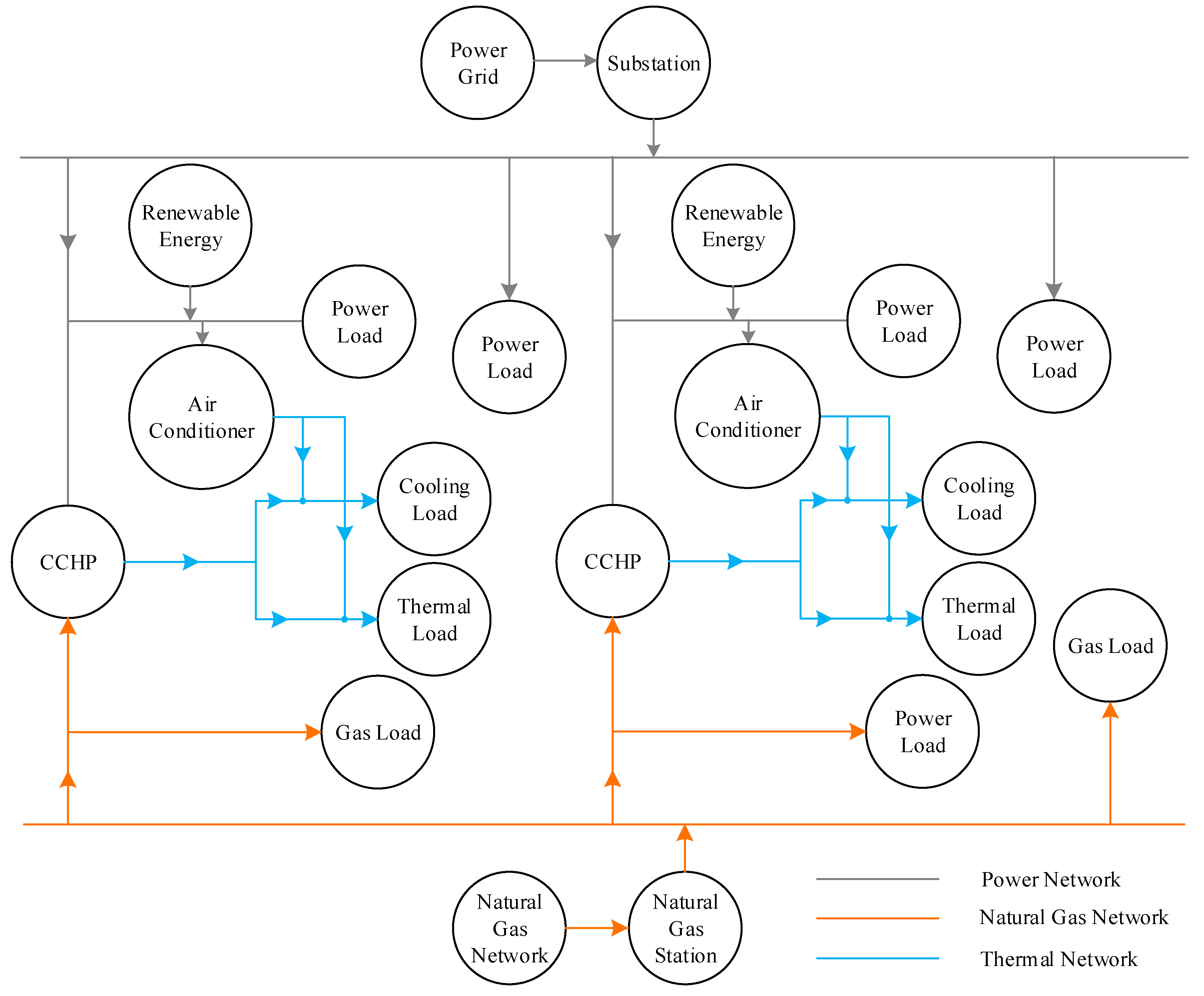
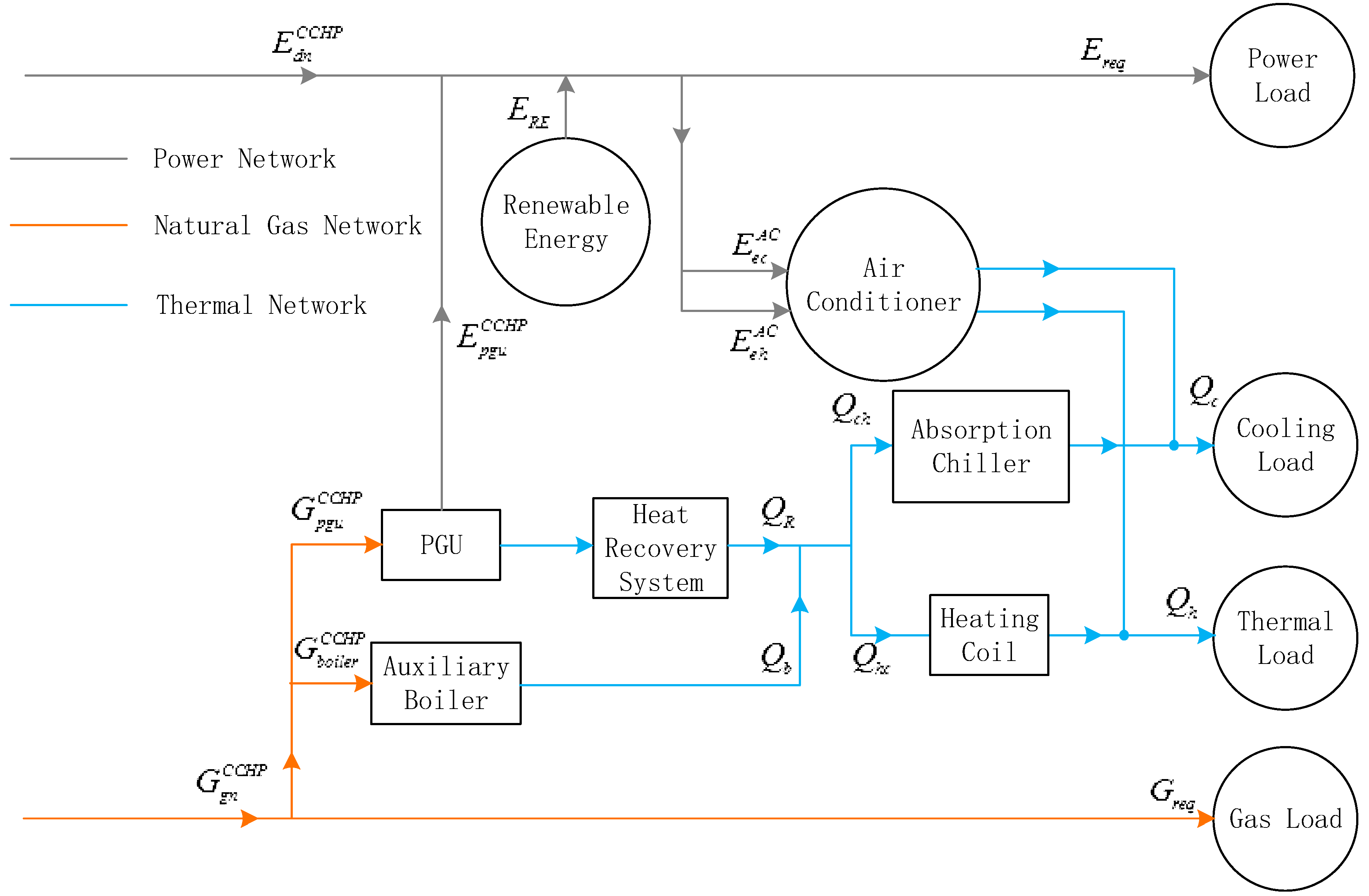
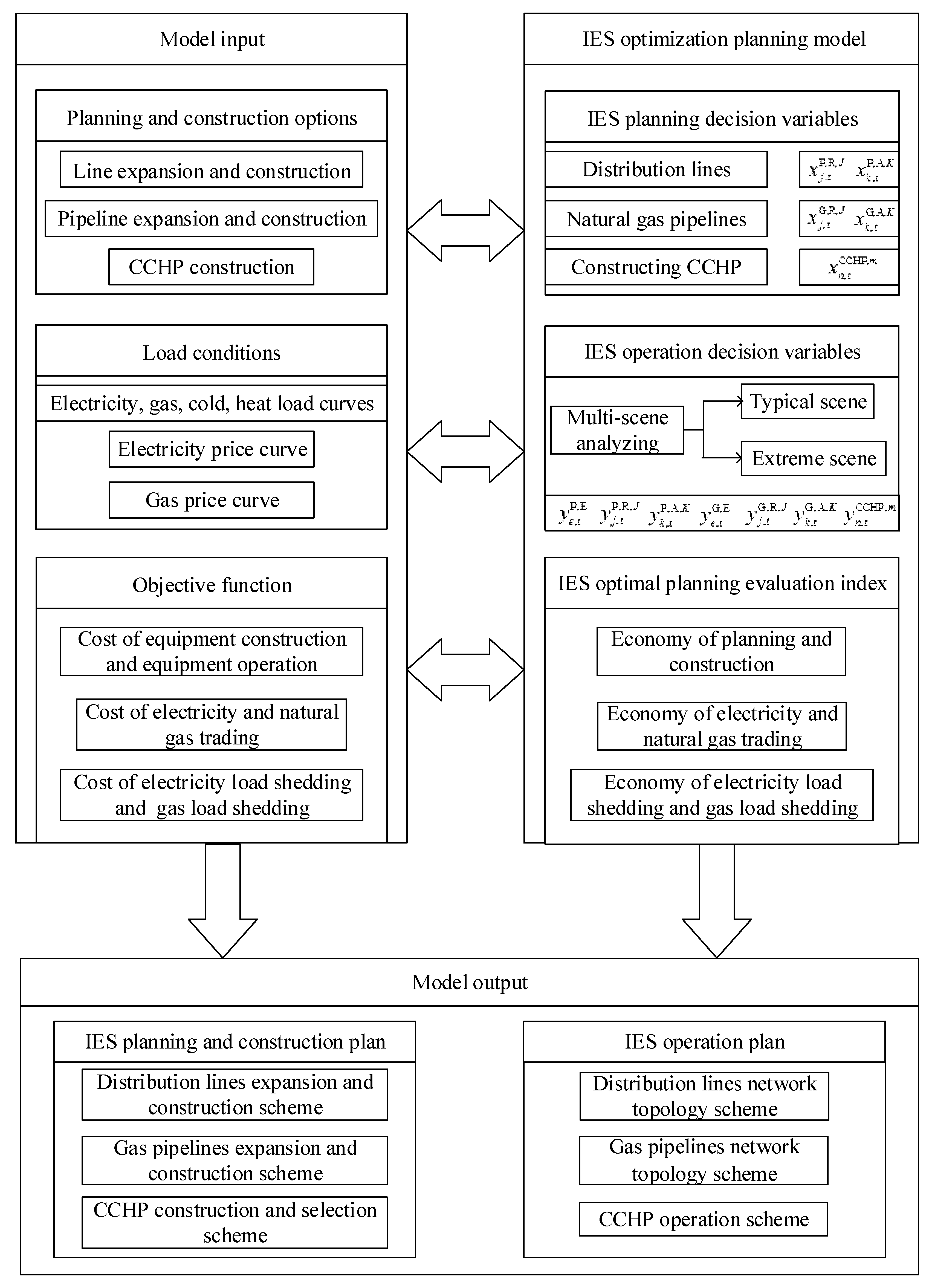
Based on the traditional expansion planning model of multistage distribution network and gas network [36] and typical CCHP system planning model [34], the IES physical programming model including distribution network, gas network and CCHP system is presented as shown in Figure 1. The CCHP physical programming model is presented as shown in Figure 2. The IES optimization programming model including model input and model output is shown in Figure 3.

In the IES physical programming model, some nodes set up the CCHP system as the electric and gas coupled hub, and the other nodes are only the electric load node or the natural gas load node. The CCHP physical programming model describes the connection and energy flow relation of gas turbine, auxiliary gas boiler, heat recovery system, absorption chiller and heating coil in the CCHP system, and how to cooperate with electric air conditioner and renewable energy power generation to output cold and heat load. The optimization objective of this paper is to minimize the total investment and operation cost of IES. Transmission lines or pipes that transmit electricity, gas, cold and heat from nodes to customers are not considered. This part of the line or pipeline is common to different planning models. It is located within the user and depends on the design of the user’s architecture. It usually does not change with the external planning.

The IES optimization programming model contains 3 parts:

(1) Model input:

(a)

The IES planning and construction options include: The distribution line expansion and construction options, the gas pipeline expansion and construction options and the CCHP construction options.

(b)

The load conditions of IES operation include: The electricity, gas, cold and heat load curves of nodes, and the electricity and gas price curves.

(c)

IES objective function weights include: The unit distance cost of distribution line, gas pipeline, the unit power cost of CCHP, and maintenance cost, the per kilowatt hour cost of power, the per cubic meter cost of natural gas, the unit power cost of electricity and gas load shedding with corresponding conversion coefficient.

(2) The objective function is added in accordance with each weight value. The economy of planning and construction, the economy of electricity and natural gas trading, and the economy of electricity load shedding and gas load shedding are obtained. The decision variables are divided into two categories:

(a)

Planning decision variables include replacing existing distribution lines ($x_{j,t}^{\mathrm{P},\mathrm{R},J}$), adding new distribution lines ($x_{k,t}^{\mathrm{P},\mathrm{A},K}$), replacing existing natural gas pipelines ($x_{j,t}^{\mathrm{G},\mathrm{R},J}$), adding new natural gas pipelines ($x_{k,t}^{\mathrm{G},\mathrm{A},K}$) and constructing CCHP systems ($x_{n,t}^{\mathrm{CCH}\mathrm{P},m}$).

(b)

Operation decision variables include the operating state ($y_t$) of the power distribution lines, gas pipelines and CCHP systems in the IES, the power level (${\mathit{E}}_{h,s,t}^{\mathrm{SUB}}$) of electricity load in the IES system and the flow level (${\mathit{\Psi }}_{h,s,t}^{\mathrm{SUB}}$) of the natural gas load.

(3) Model output:

(a)

IES planning and construction plan includes distribution lines expansion and construction scheme, gas pipelines expansion and construction scheme, CCHP construction and selection scheme.

(b)

IES operation plan includes CCHP operation scheme and IES network topology scheme under different types of daily load scenarios.

2.2. Objective

The main objective of the optimization model proposed in this paper is to get the minimum cost of the construction and operation of IES in multistage planning. Therefore, the objective function includes many aspects:

(1)

IES construction costs include the distribution line construction cost $C_{\mathrm{LI}}$, the gas pipeline construction cost $C_{\mathrm{PI}}$ and the CCHP construction cost $C_{\mathrm{CCHP}}$.

(2)

IES operation costs include the distribution line operation cost $O_{\mathrm{LI}}$, the gas pipeline operation cost $O_{\mathrm{PI}}$ and the CCHP operation cost $O_{\mathrm{CCHP}}$.

(3)

Energy transaction costs include electricity transaction cost $C_{\mathrm{PT}}$ and natural gas transaction cost $C_{\mathrm{GT}}$.

(4)

Shedding load costs include shedding electricity load cost $C_{\mathrm{CLPL}}$ and shedding gas load cost $C_{\mathrm{CLGL}}$.

The objective functions obtained from the above four costs are as follows:

$${\displaystyle \sum _t\frac{1}{{(1+i)}^{t-1}}(}{C}_{\mathrm{LI}}+C_{\mathrm{PI}}+C_{\mathrm{CCHP}})+{\displaystyle \sum _T\frac{1}{{(1+\lambda )}^{T-1}}}(O_{\mathrm{LI}}+O_{\mathrm{PI}}+O_{\mathrm{CCHP}}+C_{\mathrm{PT}}+C_{\mathrm{GT}}+C_{\mathrm{CLPL}}+C_{\mathrm{CLGL}})$$

(1)

where,

$$C_{\mathrm{LI}}={\displaystyle \sum _{j\in {\Pi }^{\mathrm{RL}}}{\displaystyle \sum _{J\in {\Omega }_j^{\mathrm{SRL}}}{C}_{\mathrm{RL},j}^J\cdot x_{j,t}^{\mathrm{P},\mathrm{R},J}}}+{\displaystyle \sum _{k\in {\Pi }^{\mathrm{AL}}}{\displaystyle \sum _{K\in {\Omega }_k^{\mathrm{SAL}}}{C}_{\mathrm{AL},k}^K\cdot x_{k,t}^{\mathrm{P},\mathrm{A},K}}}$$

(2)

$$C_{\mathrm{PI}}={\displaystyle \sum _{j\in {\Pi }^{\mathrm{RP}}}{\displaystyle \sum _{J\in {\Omega }_j^{\mathrm{SRP}}}{C}_{\mathrm{RP},j}^J\cdot x_{j,t}^{\mathrm{G},\mathrm{R},J}}}+{\displaystyle \sum _{k\in {\Pi }^{\mathrm{AP}}}{\displaystyle \sum _{K\in {\Omega }_k^{\mathrm{SAP}}}{C}_{\mathrm{AP},k}^K\cdot x_{k,t}^{\mathrm{G},\mathrm{A},K}}}$$

(3)

$$C_{\mathrm{CCHP}}={\displaystyle \sum _{n\in {\Pi }^{\mathrm{CCHP}}}{\displaystyle \sum _{m\in {\Omega }_n^{\mathrm{CCHP}}}{C}_{\mathrm{P},n,m}^{\mathrm{CCHP}}\cdot x_{n,t}^{\mathrm{CCHP},m}}}$$

(4)

$$O_{\mathrm{LI}}={\displaystyle \sum _{e\in {\Pi }^{\mathrm{EL}}}{O}_{\mathrm{EL},e}\cdot y_{e,t}^{\mathrm{P},\mathrm{E}}}+{\displaystyle \sum _{k\in {\Pi }^{\mathrm{AL}}}{\displaystyle \sum _{K\in {\Omega }_k^{\mathrm{SAL}}}{O}_{\mathrm{AL},k}^K\cdot y_{k,t}^{\mathrm{P},\mathrm{A},K}}}+{\displaystyle \sum _{j\in {\Pi }^{\mathrm{RL}}}(O_{\mathrm{RL},j}^0\cdot y_{j,t}^{\mathrm{P},\mathrm{R},0}+{\displaystyle \sum _{J\in {\Omega }_j^{\mathrm{SRL}}}{O}_{\mathrm{RL},j}^J\cdot y_{j,t}^{\mathrm{P},\mathrm{R},J}})}$$

(5)

$$O_{\mathrm{PI}}={\displaystyle \sum _{e\in {\Pi }^{\mathrm{EP}}}{O}_{\mathrm{EP},e}\cdot y_{e,t}^{\mathrm{G},\mathrm{E}}}+{\displaystyle \sum _{k\in {\Pi }^{\mathrm{AP}}}{\displaystyle \sum _{K\in {\Omega }_k^{\mathrm{SAP}}}{O}_{\mathrm{AP},k}^K\cdot y_{k,t}^{\mathrm{G},\mathrm{A},K}}+}{\displaystyle \sum _{j\in {\Pi }^{\mathrm{RP}}}(O_{\mathrm{RP},j}^0\cdot y_{j,t}^{\mathrm{G},\mathrm{R},0}+{\displaystyle \sum _{J\in {\Omega }_j^{\mathrm{SRP}}}{O}_{\mathrm{RP},j}^J\cdot y_{j,t}^{\mathrm{G},\mathrm{R},J}})}$$

(6)

$$O_{\mathrm{CCHP}}={\displaystyle \sum _{n\in {\Pi }^{\mathrm{CCHP}}}{\displaystyle \sum _{m\in {\Omega }_n^{\mathrm{CCHP}}}{O}_{\mathrm{P},n,m}^{\mathrm{CCHP}}\cdot y_{n,t}^{\mathrm{CCHP},m}}}$$

(7)

$$C_{\mathrm{PT}}={\displaystyle \sum _s{\rho }_{s,T}{\displaystyle \sum _h{P}_{\mathrm{E},h,s,T}^{\mathrm{SUB}}{\displaystyle \sum _{n\in P_{\mathrm{SN}}}{g}_{n,h,s,T}^{\mathrm{SUB}}}}}$$

(8)

$$C_{\mathrm{GT}}={\displaystyle \sum _s{\rho }_{s,T}{\displaystyle \sum _h{P}_{\mathrm{G},h,s,T}^{\mathrm{SUB}}{\displaystyle \sum _{n\in G_{\mathrm{SN}}}{\mathit{\Psi }}_{n,h,s,T}^{\mathrm{SUB}}}}}$$

(9)

$$C_{\mathrm{CLPL}}=C_{\mathrm{LP}}{\displaystyle \sum _T({\displaystyle \sum _h{r}_{e,h,T}^{\mathrm{P}}+{\displaystyle \sum _s{\displaystyle \sum _h{r}_{s,h,T}^{\mathrm{P}}}}})}$$

(10)

$$C_{\mathrm{CLGL}}=C_{\mathrm{LG}}{\displaystyle \sum _T({\displaystyle \sum _h{r}_{e,h,T}^{\mathrm{G}}+{\displaystyle \sum _s{\displaystyle \sum _h{r}_{s,h,T}^{\mathrm{G}}}}})}$$

(11)

$C_{\mathrm{LP}}$ represents the cost of per unit power load shedding. $C_{\mathrm{LG}}$ represents the cost of per unit gas load shedding. $r_{e,h,T}^{\mathrm{P}}$ and $r_{s,h,T}^{\mathrm{P}}$ represent the h hour power load shedding under extreme day scenario and typical day scenario. $r_{e,h,T}^{\mathrm{G}}$ and $r_{s,h,T}^{\mathrm{G}}$ represent the h hour gas load shedding under extreme day scenario and typical day scenario. In the modeling, a large numerical value of the load shedding coefficient is set. Optimization program to minimize the objective function will avoid the appearance of load shedding during the operation. The appearance of the cost indicates that the construction plan does not meet the load requirements and the planning and construction plan should be readjusted.

2.3. Distribution Network Constraints

Reference [37] proposed a distribution network expansion planning model with distributed power supplying and energy storage based on Kirchhoff’s law. The problem of this paper is related to the corresponding distribution network planning constraints. Based on the above model, the conventional constraints of distribution network are modified and expanded accordingly.

(1) Power balance and power limits (KCL)

$${\mathit{f}}_{h,s,t}^{\mathrm{SUB}}+{\mathit{f}}_{\mathrm{pgu},h,s,t}^{\mathrm{CCHP}}+{\mathit{r}}_{h,s,t}^{\mathrm{P}}={\mathit{S}}^{\mathrm{EL}}{\mathit{f}}_{h,s,t}^{\mathrm{E}}+{\mathit{S}}^{\mathrm{RL}}{\mathit{f}}_{h,s,t}^{\mathrm{R}}+{\mathit{S}}^{\mathrm{AL}}{\mathit{f}}_{h,s,t}^{\mathrm{A}}+{\mathit{f}}_{\mathrm{rep},h,s,t}+{\mathit{f}}_{\mathrm{ec},h,s,t}+{\mathit{f}}_{\mathrm{eh},h,s,t}$$

(12)

In (12), ${\mathit{f}}_{}^{\mathrm{SUB}}$, ${\mathit{f}}_{\mathrm{pgu}}^{\mathrm{CCHP}}$, ${\mathit{r}}_{}^{\mathrm{P}}$, ${\mathit{f}}_{\mathrm{rep}}$, ${\mathit{f}}_{\mathrm{ec}}$, ${\mathit{f}}_{\mathrm{eh}}$ represent the current vector form of substation injection power, CCHP generation power, node power load shedding, node electric load power, electric air conditioner refrigeration power and electric air conditioner heat power. The above variables form an equation through the nodal incidence matrix (${\mathit{S}}^{\mathrm{EL}}$, ${\mathit{S}}^{\mathrm{RL}}$, ${\mathit{S}}^{\mathrm{AL}}$) and the branch current vector (${\mathit{f}}_{}^{\mathrm{E}}$, ${\mathit{f}}_{}^{\mathrm{R}}$, ${\mathit{f}}_{}^{\mathrm{A}}$).

(2) Nodal voltage calculation and limits (KVL)

$$|Z_j^{\mathrm{R},0}{f}_{j,h,s,t}^{\mathrm{R}}-{[{\mathit{S}}^{\mathrm{RL}}]}_{rowj}^{\mathrm{T}}{\mathit{V}}_{h,s,t}|\le M(1-y_{j,h,s,t}^{\mathrm{P},\mathrm{R},0}),\forall j\in {\Pi }^{\mathrm{RL}}$$

(13)

$$|Z_j^{\mathrm{R},J}{f}_{j,h,s,t}^{\mathrm{R}}-{[{\mathit{S}}^{\mathrm{RL}}]}_{rowj}^{\mathrm{T}}{\mathit{V}}_{h,s,t}|\le M(1-y_{j,h,s,t}^{\mathrm{P},\mathrm{R},J}),\forall j\in {\Pi }^{\mathrm{RL}},J\in {\Omega }_j^{\mathrm{SRL}}$$

(14)

$$|Z_k^{\mathrm{A},K}{f}_{k,h,s,t}^{\mathrm{A}}-{[{\mathit{S}}^{\mathrm{AL}}]}_{rowk}^{\mathrm{T}}{\mathit{V}}_{h,s,t}|\le M(1-y_{k,h,s,t}^{\mathrm{P},\mathrm{A},K}),\forall k\in {\Pi }^{\mathrm{AL}},K\in {\Omega }_k^{\mathrm{SAL}}$$

(15)

$$|Z_e^{\mathrm{E}}{f}_{e,h,s,t}^{\mathrm{E}}-{[{\mathit{S}}^{\mathrm{EL}}]}_{rowe}^{\mathrm{T}}{\mathit{V}}_{h,s,t}|\le M(1-y_{e,h,s,t}^{\mathrm{P},\mathrm{E}}),\forall e\in {\Pi }^{\mathrm{EL}}$$

(16)

$$V_{\min }\le V_{h,s,t}\le V_{\max }$$

(17)

Z and f are the impedance and current values of the corresponding type distribution lines, respectively. V is the node voltage column vector. The subscript row j represents the j column. M is a large enough positive number. When the distribution line does not run (y = 0), the inequality is relaxed. When the distribution line runs (y = 1), the inequality becomes the equation to calculate the corresponding node voltage. The node voltage is constrained in (17).

(3) Maximum load constraint of distribution line

$$|f_{e,h,s,t}^{\mathrm{E}}|\le y_{e,t}^{\mathrm{P},\mathrm{E}}{f}_{e,\max }^{\mathrm{E}}\hspace{1em}\forall e\in {\Pi }^{\mathrm{EL}}$$

(18)

$$|f_{j,h,s,t}^{\mathrm{R}}|\le y_{j,t}^{\mathrm{P},\mathrm{R},0}{f}_{j,\max }^{\mathrm{R},0}+{\displaystyle \sum _{J\in {\Omega }_j^{\mathrm{SRL}}}{y}_{j,t}^{\mathrm{P},\mathrm{R},J}{f}_{j,\max }^{\mathrm{R},J}}\hspace{1em}\forall j\in {\Pi }^{\mathrm{RL}}$$

(19)

$$|f_{k,h,s,t}^{\mathrm{A}}|\le {\displaystyle \sum _{K\in {\Omega }_k^{\mathrm{SAL}}}{y}_{k,t}^{\mathrm{P},\mathrm{A},K}{f}_{k,\max }^{\mathrm{A},K}}\hspace{1em}\forall k\in {\Pi }^{\mathrm{AL}}$$

(20)

(4) Power constraint in substation

$$0\le f_{n,h,s,t}^{\mathrm{SUB}}\le f_{n,\max }^{\mathrm{SUB}}\hspace{1em}\forall n\in P_{\mathrm{SN}}$$

(21)

(5) Power load shedding constraint

$$0\le r_{n,h,s,t}^{\mathrm{P}}\le f_{\mathrm{rep},n,h,s,t}\hspace{1em}\forall n\in P_{\mathrm{LN}}$$

(22)

All constraints mentioned above are set up at any planning time t, any typical day scenario s, and any time point h in formula (12)–(22).

(6) Logic constraint of distribution line construction

During all the planning periods, only one expansion or new construction is considered for the same line, and the following constraints are obtained.

$${\displaystyle \sum _t{\displaystyle \sum _{J\in {\Omega }_j^{\mathrm{SRL}}}{x}_{j,t}^{\mathrm{P},\mathrm{R},J}}}\le 1,\hspace{1em}\forall j\in {\Pi }^{\mathrm{RL}}$$

(23)

$${\displaystyle \sum _t{\displaystyle \sum _{K\in {\Omega }_k^{\mathrm{SAL}}}{x}_{k,t}^{\mathrm{P},\mathrm{A},K}}}\le 1,\hspace{1em}\forall k\in {\Pi }^{\mathrm{AL}}$$

(24)

After the expansion of the replacement line and the construction of the new line, the corresponding lines will be put into use, thus the following constraints are obtained.

$$y_{j,t}^{\mathrm{P},\mathrm{R},J}\le {\displaystyle \sum _{t^{\prime }=1}^t{x}_{j,t^{\prime }}^{\mathrm{P},\mathrm{R},J}}\hspace{1em}\forall t,\forall j\in {\Pi }^{\mathrm{RL}},\forall J\in {\Omega }_j^{\mathrm{SRL}}$$

(25)

$$y_{k,t}^{\mathrm{P},\mathrm{A},K}\le {\displaystyle \sum _{t^{\prime }=1}^t{x}_{k,t^{\prime }}^{\mathrm{P},\mathrm{A},K}}\hspace{1em}\forall t,\forall k\in {\Pi }^{\mathrm{AL}},\forall K\in {\Omega }_k^{\mathrm{SAL}}$$

(26)

After the expansion line is completed, the original lines are no longer used, and the following constraints are obtained.

$$y_{j,t}^{\mathrm{P},\mathrm{R},0}\le 1-{\displaystyle \sum _{t^{\prime }=1}^t{\displaystyle \sum _{J\in {\Omega }_j^{\mathrm{SRL}}}{x}_{j,t^{\prime }}^{\mathrm{P},\mathrm{R},J}}}\hspace{1em}\forall t,\forall j\in {\Pi }^{\mathrm{RL}}$$

(27)

(7) Spanning tree constraint

The distribution network in this paper is a radial network, so it is necessary to consider the spanning tree constraint to ensure that the topology of the distribution network is a radial network. The spanning tree has the following 3 kinds of characters.

① The number of non-root nodes is equal to the number of branches in operation.

② For any branch, the nodes at both ends satisfy the “parent node” relationship.

③ For any non-root node, its “parent node” is unique, and root node has no “parent node” [38].

Spanning tree constraints satisfy the following equality constraints.

$${\alpha }_{e,t}^{\mathrm{P},\mathrm{E}}=y_{e,t}^{\mathrm{P},\mathrm{E}}$$

(28)

$${\alpha }_{j,t}^{\mathrm{P},\mathrm{R}}=y_{j,t}^{\mathrm{P},\mathrm{R},0}+{\displaystyle \sum _{J\in {\Omega }_j^{\mathrm{SRL}}}{y}_{j,t}^{\mathrm{P},\mathrm{R},J}}$$

(29)

$${\alpha }_{k,t}^{\mathrm{P},\mathrm{A}}={\displaystyle \sum _{K\in {\Omega }_k^{\mathrm{SAL}}}{y}_{k,t}^{\mathrm{P},\mathrm{A},K}}$$

(30)

$${\alpha }_{e,t}^{\mathrm{P},\mathrm{E}}={\beta }_{e,t}^{\mathrm{P},+,\mathrm{E}}+{\beta }_{e,t}^{\mathrm{P},-,\mathrm{E}}$$

(31)

$${\alpha }_{j,t}^{\mathrm{P},\mathrm{R}}={\beta }_{j,t}^{\mathrm{P},+,\mathrm{R}}+{\beta }_{j,t}^{\mathrm{P},-,\mathrm{R}}$$

(32)

$${\alpha }_{k,t}^{\mathrm{P},\mathrm{A}}={\beta }_{k,t}^{\mathrm{P},+,\mathrm{A}}+{\beta }_{k,t}^{\mathrm{P},-,\mathrm{A}}$$

(33)

$${\displaystyle \sum _{n\in P_{\mathrm{LN}}}({\beta }_{e,t}^{\mathrm{P},\mathrm{back},\mathrm{E}}+{\beta }_{j,t}^{\mathrm{P},\mathrm{back},\mathrm{R}}+{\beta }_{k,t}^{\mathrm{P},\mathrm{back},\mathrm{A}})}=1$$

(34)

$${\displaystyle \sum _{n\in P_{\mathrm{SN}}}({\beta }_{e,t}^{\mathrm{P},\mathrm{back},\mathrm{E}}+{\beta }_{j,t}^{\mathrm{P},\mathrm{back},\mathrm{R}}+{\beta }_{k,t}^{\mathrm{P},\mathrm{back},\mathrm{A}})}=0$$

(35)

The 0-1 variable $\alpha$ in Equations (28)–(30) is used to indicate whether the line exists in spanning tree topology. The 0-1 variables ${\beta }_{}^{\mathrm{P},+}$ and ${\beta }_{}^{\mathrm{P},-}$ in Equations (31)–(33) indicate “parent node” relationship at both ends of the branch. ${\beta }_{}^{\mathrm{P},+}$ represents a positive direction along the branch. Equations (34) and (35) indicate the parent node of the load node exists and is unique. There is not parent node in substation node. ${\beta }_{}^{\mathrm{P},\mathrm{back}}$ represents the back to this node in the branch. Its value is ${\beta }_{}^{\mathrm{P},+}$ or ${\beta }_{}^{\mathrm{P},-}$.

If the network has 1, 2, 3 three nodes, we suppose the branch direction is 1-2-3. The node 3 is the root node, and the node 2 is the parent node of node 1. We suppose the direction of the branch is the positive direction. The branch of 1-2 is the branch 1, and the branch of 2-3 is the branch 2. For node 2, the direction of the back to node 2 is opposite to the positive direction of branch 1 and is the same direction as the positive direction of branch 2. That is, ${\beta }_1^{\mathrm{P},\mathrm{back}}$ = ${\beta }_1^{\mathrm{P},-}$ = 0, ${\beta }_2^{\mathrm{P},\mathrm{back}}$ = ${\beta }_2^{\mathrm{P},+}$ = 1, therefore, ${\beta }_1^{\mathrm{P},\mathrm{back}}$ + ${\beta }_2^{\mathrm{P},\mathrm{back}}$ = 1. For node 3, the direction of the back to node 3 is opposite to the positive direction of branch 2. That is, ${\beta }_2^{\mathrm{P},\mathrm{back}}$ = ${\beta }_2^{\mathrm{P},-}$ = 0.

2.4. Gas Pipe Network Constraint

Gas pipe network constraints mainly consider natural gas node flow balance constraints, gas pipeline flow and pressure relationship constraints, flow constraints of gas pipeline, natural gas station, gas load shedding and construction logic constraints of gas pipeline.

(1) Flow balance constraint of natural gas node

$${\mathit{\Psi }}_{h,s,t}^{\mathrm{SUB}}+{\mathit{\Psi }}_{\mathrm{r},h,s,t}^{\mathrm{G}}={\mathit{S}}^{\mathrm{EP}}{\mathit{\Psi }}_{h,s,t}^{\mathrm{E}}+{\mathit{S}}^{\mathrm{RP}}{\mathit{\Psi }}_{h,s,t}^{\mathrm{R}}+{\mathit{S}}^{\mathrm{AP}}{\mathit{\Psi }}_{h,s,t}^{\mathrm{A}}+{\mathit{\Psi }}_{\mathrm{pgu},h,s,t}^{\mathrm{CCHP}}+{\mathit{\Psi }}_{\mathrm{boiler},h,s,t}^{\mathrm{CCHP}}+{\mathit{\Psi }}_{\mathrm{rep},h,s,t}$$

(36)

In (36), ${\mathit{\Psi }}_{}^{\mathrm{SUB}}$, ${\mathit{\Psi }}_{\mathrm{r}}^{\mathrm{G}}$, ${\mathit{\Psi }}_{\mathrm{pgu}}^{\mathrm{CCHP}}$, ${\mathit{\Psi }}_{\mathrm{boiler}}^{\mathrm{CCHP}}$, ${\mathit{\Psi }}_{\mathrm{rep}}$ represent the vector form of natural gas station injection flow, node gas load shedding flow, gas flow consumed by CCHP gas turbine, gas flow consumed by CCHP auxiliary gas boiler, node gas load flow. The above variables form an equation through the nodal incidence matrix (${\mathit{S}}^{\mathrm{EP}}$, ${\mathit{S}}^{\mathrm{RP}}$, ${\mathit{S}}^{\mathrm{AP}}$) and the branch flow vector (${\mathit{\Psi }}_{}^{\mathrm{E}}$, ${\mathit{\Psi }}_{}^{\mathrm{R}}$, ${\mathit{\Psi }}_{}^{\mathrm{A}}$).

(2) Natural gas flow-pressure relation and pressure amplitude constraint

The relationship between the flow of natural gas pipeline and the pressure of the node is

$$\mathrm{sign}({\Psi }_{ij}){\Psi }_{ij}^2=C_{ij}^2(p_i^2-p_j^2)=C_{ij}^2(P_i-P_j)$$

(37)

In (37), ${\Psi }_{ij}$ represents natural gas flow from node i to node j. $C_{ij}^2$ represents pipeline constant of i-j gas pipeline. $p_i$ represents gas absolute pressure of node i. $p_j$ represents gas absolute pressure of node j. $P_i$ represents the square of gas absolute pressure of node i. $P_j$ represents the square of gas absolute pressure of node j.

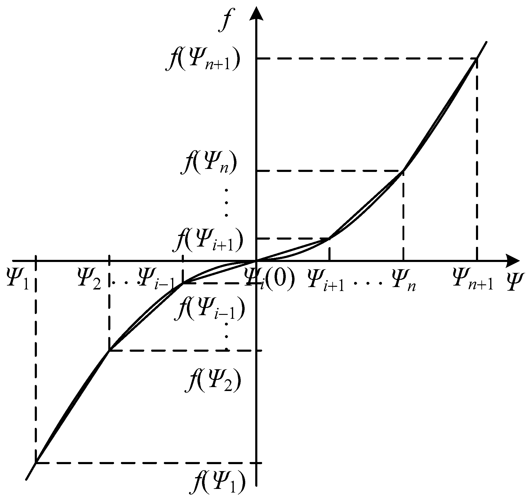
Because MILP is adopted in the optimization model, there are only linear constraints in the constraint conditions. For nonlinear constraints in (37), piecewise linearization is required, as shown in Figure 4.

In (37), the function on the leftmost side of the equation is a nonlinear function. Suppose $f=\mathrm{sign}({\Psi }_{ij}){\Psi }_{ij}^2$ and the function curve is divided into a linear combination of N segments. The points of each subsection are ${\Psi }_1\le {\Psi }_2\le \cdots$ $\le {\Psi }_i\le \cdots$ ${\Psi }_n\le {\Psi }_{n+1}$. Introduce a new variable $z_k$. The piecewise linear function $f_{\mathrm{linear}}$ and natural gas pipeline flow $\Psi$ are respectively expressed as

$$f_{\mathrm{linear}}(\Psi )={\displaystyle \sum _{k=1}^{n+1}{z}_{k}f({\Psi }_k)}$$

(38)

$$\Psi ={\displaystyle \sum _{k=1}^{n+1}{z}_k{\Psi }_k}$$

(39)

Reintroduce a new 0-1 variable $y_k$. The relationship between $z_k$ and $y_k$ meets the following constraints.

$$z_1\le y_1,z_2\le y_1+y_2,\cdots z_n\le y_{n-1}+y_n,z_{n+1}\le y_n$$

(40)

$$y_1+y_2+\cdots +y_n=1,y_k=0,1$$

(41)

$$z_1+z_2+\cdots +z_n=1,z_k\ge 0,k=1,2,\cdots ,n+1$$

(42)

According to the above steps, the nonlinear constraints can be transformed into linear constraints. In (37), the relationship between natural gas flow and pressure can be transformed into the following constraints.

$$|{\displaystyle \sum _{k=1}^{n+1}{z}_k^{\mathrm{R},0}f({\Psi }_{k,j,h,s,t}^{\mathrm{R}})}-C_{j,\mathrm{R},0}^2{[{\mathit{S}}^{\mathrm{RP}}]}_{\mathrm{row}j}^{\mathrm{T}}{\mathit{P}}_{h,s,t}|\le M(1-y_{j,h,s,t}^{\mathrm{G},\mathrm{R},0})\hspace{1em}\forall j\in {\Pi }^{\mathrm{RP}}$$

(43)

$$|{\displaystyle \sum _{k=1}^{n+1}{z}_k^{\mathrm{R},J}f({\Psi }_{k,j,h,s,t}^{\mathrm{R}})}-C_{j,\mathrm{R},J}^2{[{\mathit{S}}^{\mathrm{RP}}]}_{\mathrm{row}j}^{\mathrm{T}}{\mathit{P}}_{h,s,t}|\le M(1-y_{j,h,s,t}^{\mathrm{G},\mathrm{R},J})\hspace{1em}\forall j\in {\Pi }^{\mathrm{RP}},J\in {\Omega }_j^{\mathrm{SRP}}$$

(44)

$$|{\displaystyle \sum _{k=1}^{n+1}{z}_k^{\mathrm{A},K}f({\Psi }_{k,k,h,s,t}^{\mathrm{A}})}-C_{k,\mathrm{A},K}^2{[{\mathit{S}}^{\mathrm{AP}}]}_{rowk}^{\mathrm{T}}{\mathit{P}}_{h,s,t}|\le M(1-y_{k,h,s,t}^{\mathrm{G},\mathrm{A},K})\hspace{1em}\forall k\in {\Pi }^{\mathrm{AP}},K\in {\Omega }_k^{\mathrm{SAP}}$$

(45)

$$|{\displaystyle \sum _{k=1}^{n+1}{z}_k^{\mathrm{E}}f({\Psi }_{k,e,h,s,t}^{\mathrm{E}})}-C_{e,\mathrm{E}}^2{[{\mathit{S}}^{\mathrm{EP}}]}_{rowe}^{\mathrm{T}}{\mathit{P}}_{h,s,t}|\le M(1-y_{e,h,s,t}^{\mathrm{G},\mathrm{E}})\hspace{1em}\forall e\in {\Pi }^{\mathrm{EP}}$$

(46)

$$P_{\min }\le {\mathit{P}}_{h,s,t}\le P_{\max }$$

(47)

(3) Maximum flow constraint of gas pipeline

$$|{\Psi }_{e,h,s,t}^{\mathrm{E}}|\le y_{e,t}^{\mathrm{G},\mathrm{E}}{\Psi }_{e,\max }^{\mathrm{E}}\hspace{1em}\forall e\in {\Pi }^{\mathrm{EP}}$$

(48)

$$|{\Psi }_{j,h,s,t}^{\mathrm{R}}|\le y_{j,t}^{\mathrm{G},\mathrm{R},0}{\Psi }_{j,\max }^{\mathrm{R},0}+{\displaystyle \sum _{J\in {\Omega }_j^{\mathrm{SRP}}}{y}_{j,t}^{\mathrm{G},\mathrm{R},J}{\Psi }_{j,\max }^{\mathrm{R},J}}\hspace{1em}\forall j\in {\Pi }^{\mathrm{RP}}$$

(49)

$$|{\Psi }_{k,h,s,t}^{\mathrm{A}}|\le {\displaystyle \sum _{K\in {\Omega }_k^{\mathrm{SAP}}}{y}_{k,t}^{\mathrm{G},\mathrm{A},K}{\Psi }_{k,\max }^{\mathrm{A},K}}\hspace{1em}\forall k\in {\Pi }^{\mathrm{AP}}$$

(50)

(4) Flow constraint of natural gas station

$$0\le {\Psi }_{n,h,s,t}^{\mathrm{SUB}}\le {\Psi }_{n,\max }^{\mathrm{SUB}}\hspace{1em}\forall n\in G_{\mathrm{SN}}$$

(51)

(5) flow constraint of natural gas load shedding

$$0\le {\Psi }_{\mathrm{r},n,h,s,t}^{\mathrm{G}}\le {\mathit{\Psi }}_{\mathrm{rep},n,h,s,t}\hspace{1em}\forall n\in G_{\mathrm{LN}}$$

(52)

(6) Logic constraint of gas pipeline construction

$${\displaystyle \sum _t{\displaystyle \sum _{J\in {\Omega }_j^{\mathrm{SRP}}}{x}_{j,t}^{\mathrm{G},\mathrm{R},J}}}\le 1\hspace{1em}\forall j\in {\Pi }^{\mathrm{RP}}$$

(53)

$${\displaystyle \sum _t{\displaystyle \sum _{K\in {\Omega }_k^{\mathrm{SAP}}}{x}_{k,t}^{\mathrm{G},\mathrm{A},K}}}\le 1\hspace{1em}\forall k\in {\Pi }^{\mathrm{AP}}$$

(54)

$$y_{j,t}^{\mathrm{G},\mathrm{R},J}\le {\displaystyle \sum _{t^{\prime }=1}^t{x}_{j,t^{\prime }}^{\mathrm{G},\mathrm{R},J}}\hspace{1em}\forall t,\forall j\in {\Pi }^{\mathrm{RP}},\forall J\in {\Omega }_j^{\mathrm{SRP}}$$

(55)

$$y_{k,t}^{\mathrm{G},\mathrm{A},K}\le {\displaystyle \sum _{t^{\prime }=1}^t{x}_{k,t^{\prime }}^{\mathrm{G},\mathrm{A},K}}\hspace{1em}\forall t,\forall k\in {\Pi }^{\mathrm{AP}},\forall K\in {\Omega }_k^{\mathrm{SAP}}$$

(56)

$$y_{j,t}^{\mathrm{G},\mathrm{R},0}\le 1-{\displaystyle \sum _{t^{\prime }=1}^t{\displaystyle \sum _{J\in {\Omega }_j^{\mathrm{SRP}}}{x}_{j,t^{\prime }}^{\mathrm{G},\mathrm{R},J}}}\hspace{1em}\forall t,\forall j\in {\Pi }^{\mathrm{RP}}$$

(57)

The extreme load scenario usually refers to the heaviest load period of each planning period and is used to reserve the safe boundary of the system operation. The constraints are the same as the typical day scenario.

2.5. CCHP Constraint

The relationship between devices and energy flow in CCHP is shown in Figure 2.

(1) Energy flow relationship of CCHP internal equipment

The following formulas are set up under the condition of $\forall n\in {\Pi }^{\mathrm{CCHP}}$.

$$G_{n,h,s,t}={\Psi }_{n,h,s,t}\raisebox{1ex}{$L_{cv}$}\!\left/ \!\raisebox{-1ex}{$3.6$}\right.$$

(58)

$$E_{n,h,s,t}=\sqrt{3}{V}_{\mathrm{nominal}}{f}_{n,h,s,t}$$

(59)

$$E_{\mathrm{pgu},n,h,s,t}^{\mathrm{CCHP}}=G_{\mathrm{pgu},n,h,s,t}^{\mathrm{CCHP}}{\eta }_{\mathrm{pgu}}$$

(60)

$$Q_{\mathrm{R},n,h,s,t}=G_{\mathrm{pgu},n,h,s,t}^{\mathrm{CCHP}}\left(1-{\eta }_{\mathrm{pgu}}\right){\eta }_{\mathrm{rec}}$$

(61)

$$Q_{\mathrm{b},n,h,s,t}={\mathrm{G}}_{\mathrm{boiler},n,h,s,t}^{\mathrm{CCHP}}{\eta }_{\mathrm{boiler}}$$

(62)

$$Q_{\mathrm{R},n,h,s,t}+Q_{\mathrm{b},n,h,s,t}=Q_{\mathrm{c}\mathrm{h},n,h,s,t}+Q_{\mathrm{h}\mathrm{c},n,h,s,t}$$

(63)

$$Q_{\mathrm{c},n,h,s,t}=Q_{\mathrm{c}\mathrm{h},n,h,s,t}{C}_{\mathrm{ac}}+E_{\mathrm{ec},n,h,s,t}^{\mathrm{A}\mathrm{C}}{C}_{\mathrm{ec}}$$

(64)

$$Q_{\mathrm{h},n,h,s,t}=Q_{\mathrm{h}\mathrm{c},n,h,s,t}{\eta }_{\mathrm{h}\mathrm{c}}+E_{\mathrm{eh},n,h,s,t}^{\mathrm{A}\mathrm{C}}{C}_{\mathrm{eh}}$$

(65)

(2) CCHP internal device constraints

$${\displaystyle \sum _t{\displaystyle \sum _{m\in {\Omega }_n^{\mathrm{CCHP}}}{x}_{n,t}^{\mathrm{CCHP},m}}}\le 1\hspace{1em}\forall n\in {\Pi }^{\mathrm{CCHP}}$$

(66)

$$y_{n,t}^{\mathrm{CCHP},m}\le {\displaystyle \sum _{t^{\prime }=1}^t{x}_{n,t}^{\mathrm{CCHP},m}}\hspace{1em}\forall t,\forall n\in {\Pi }^{\mathrm{CCHP}},\forall m\in {\Omega }_n^{\mathrm{CCHP}}$$

(67)

$$\begin{array}{l}{\displaystyle \sum _{m\in {\Omega }_n^{\mathrm{CCHP}}}{y}_{n,t}^{\mathrm{CCHP},m}{E}_{\mathrm{pgu},\min ,m,n,t}^{\mathrm{CCHP}}}\le E_{\mathrm{pgu},n,s,t}^{\mathrm{CCHP}}\le \\ {\displaystyle \sum _{m\in {\Omega }_n^{\mathrm{CCHP}}}{y}_{n,t}^{\mathrm{CCHP},m}{E}_{\mathrm{pgu},\max ,m,n,t}^{\mathrm{CCHP}}}\hspace{1em}\forall n\in {\Pi }^{\mathrm{CCHP}}\end{array}$$

(68)

$$\begin{array}{l}{\displaystyle \sum _{m\in {\Omega }_n^{\mathrm{CCHP}}}{y}_{n,t}^{\mathrm{CCHP},m}{G}_{\mathrm{boiler},\min ,m,n,t}^{\mathrm{CCHP}}}\le G_{\mathrm{boiler},n,s,t}^{\mathrm{CCHP}}\le \\ {\displaystyle \sum _{m\in {\Omega }_n^{\mathrm{CCHP}}}{y}_{n,t}^{\mathrm{CCHP},m}{G}_{\mathrm{boiler},\max ,m,n,t}^{\mathrm{CCHP}}}\hspace{1em}\forall n\in {\Pi }^{\mathrm{CCHP}}\end{array}$$

(69)

2.6. Renewable Energy Generation

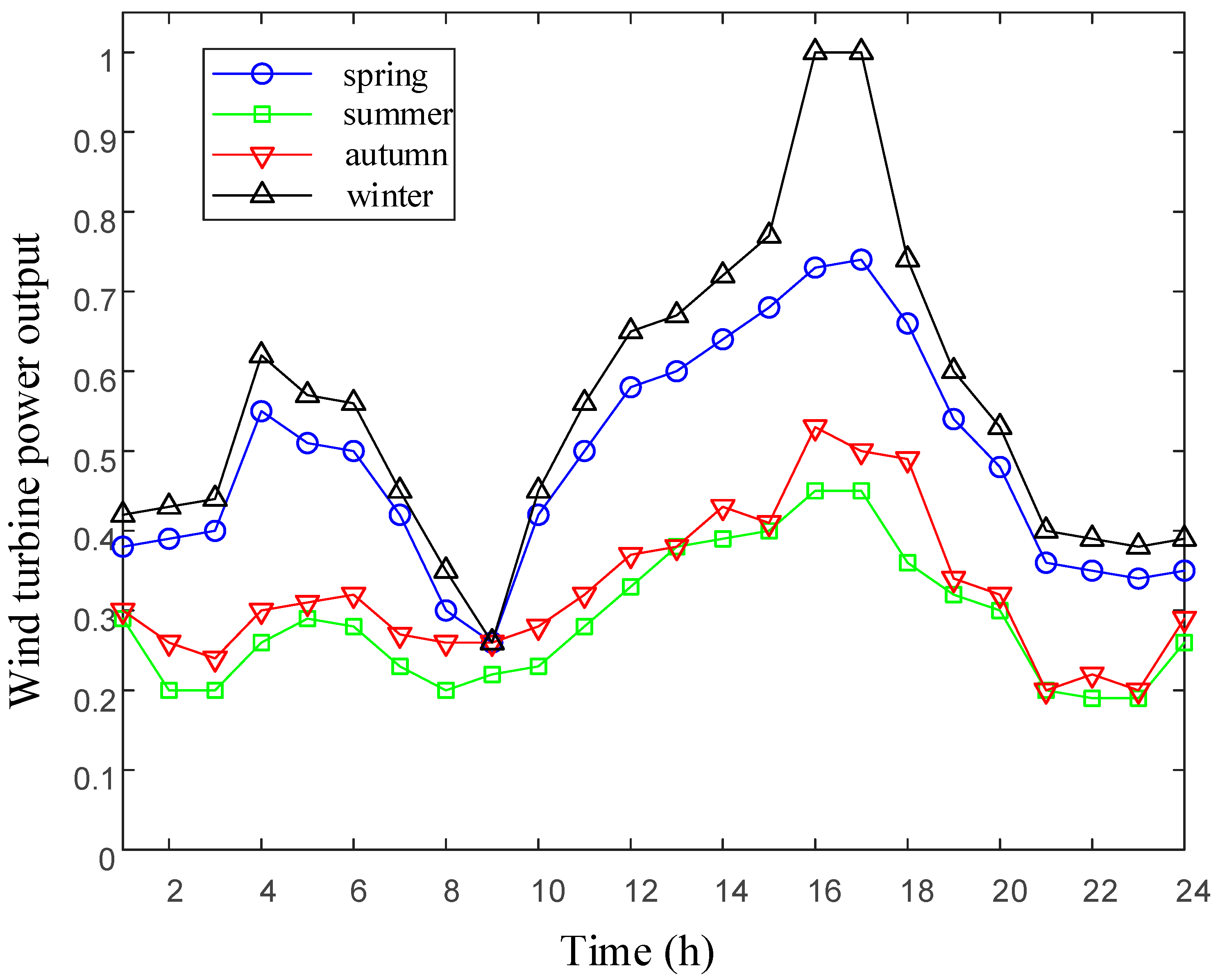
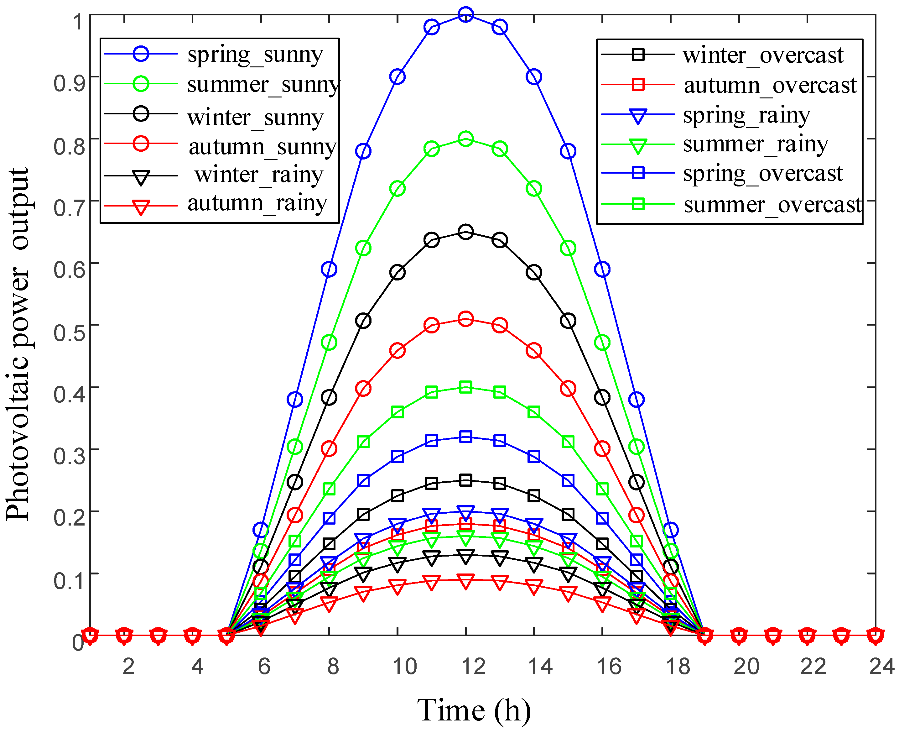
Renewable energy generation includes wind power generation and photovoltaic power generation. We need to consider the complementarity of wind and light and timing characteristic. This paper studies the 4 timing characteristics of spring, summer, autumn and winter, and models two kinds of power generation output.

The operation of wind power generation and photovoltaic power generation depends on local weather temperature and geographical environment and has high randomness and volatility. The output of wind turbines is mainly related to wind speed. The output of photovoltaic power is mainly related to the temperature and the radiance of the sun, both of which have obvious timing characteristics. Thus, the season and the weather have a great influence on wind power generation and photovoltaic power generation. There is the highest temperature and the strongest solar radiation in summer in China, so the photovoltaic power is the most. However, the wind is the weakest in summer, so the output of the wind turbine is limited. In winter, both temperature and solar radiation are low, so the output of photovoltaic power is the smallest. However, the wind is the strongest, so the output of the wind turbines is the largest. This shows that wind power and PV have very good complementarity. The photovoltaic output is greatly affected by the weather. The radiance will be greatly reduced on cloudy and rainy days, so the photovoltaic output will also be reduced at the same time. The seasonal timing characteristics of wind turbine and PV in a typical area are shown in Figure 5 and Figure 6.

According to the timing characteristic curves of wind turbine and PV, we can see that the two outputs have seasonal complementarity. In the time of the PV output of 0, the wind turbine works well. The PV output is stronger in the daytime, while the wind turbine output is weaker. So, the daily output of the two kinds of generation is complementary. Due to the randomness and volatility of photovoltaic and wind turbines, the impact of this fluctuation on the power grid can be balanced through the CCHP system.

In this paper, fixed capacity wind power generation and photovoltaic power generation are set up at relevant nodes as part of grid input. CCHP system is used to stabilize its volatility.

2.7. Model Solution

The optimization model proposed in this paper is a mixed-integer programming model. Mixed-integer programming including MILP and mixed-integer nonlinear programming (MINLP). MINLP is one of the most difficult problems in the field of planning. It belongs to the non-deterministic polynomial (NP)-hard problem. Although many scholars have carried out extensive research on MINLP problem, there is still a big gap in theory and algorithm compared with MILP problem. In addition, there are still some bottlenecks that are difficult to solve. It is difficult to determine whether the current solution is optimal or not. Therefore, this paper uses a more widely applicable MILP model, whose logic is clear, and it is easy to converge. The good scalability is beneficial to the global optimization of IES.

The optimization model is solved by MATLAB + YALMIP + GUROBI, that is, the mathematical model is established by programming tool software YALMIP in MATLAB, and the model is solved by commercial optimization solver GUROBI. The versions of software are MATLAB 2017b, YALMIP 20180612 and GUROBI 7.5.2. The CPU of desktop is Intel Core i5-4440 3.10 GHz with 8.00 GB RAM. The computational time of the easy example is about 60 min, and the relative error between the optimal feasible solution and the optimal solution is 1%.

3. Results

3.1. Case Conditions

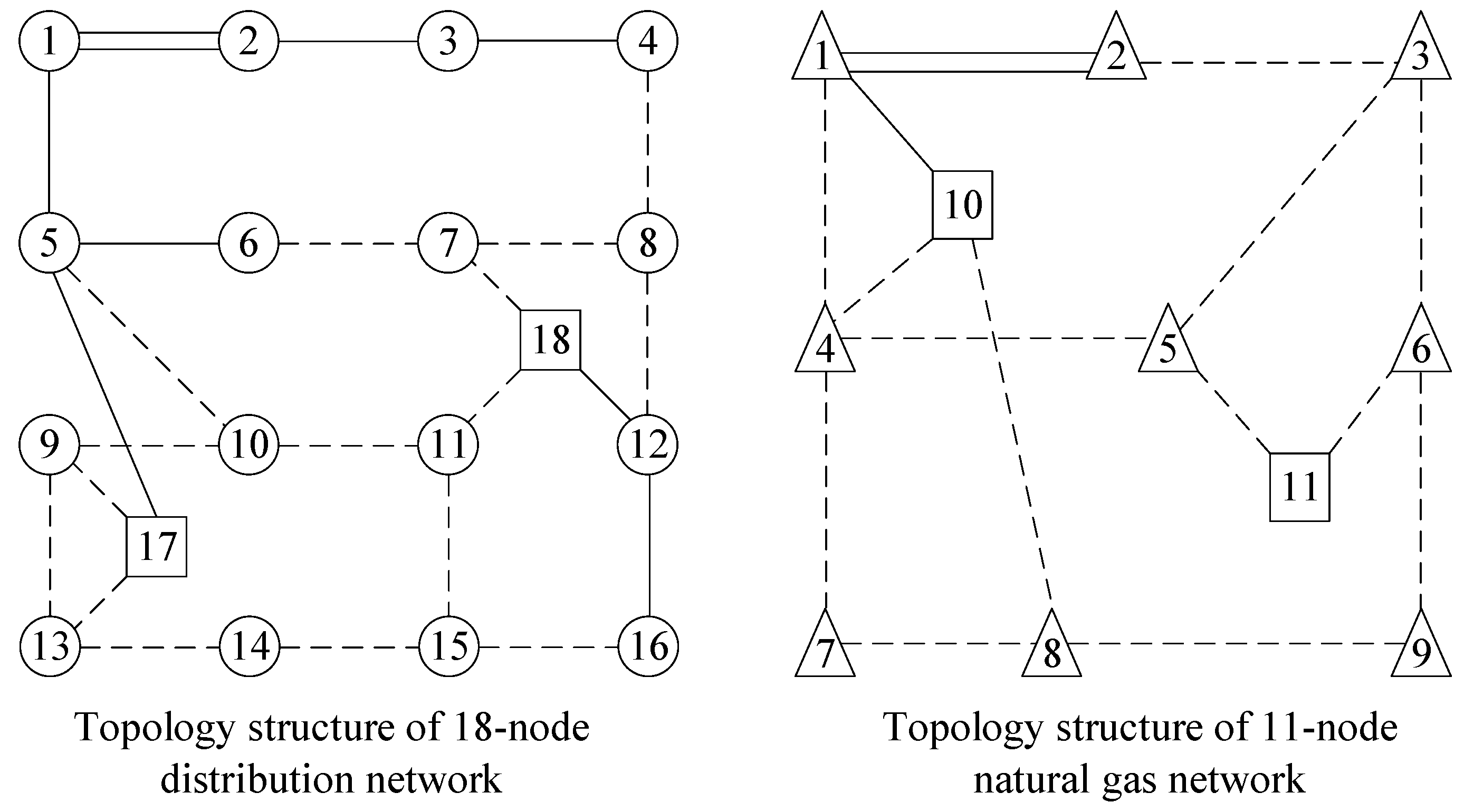
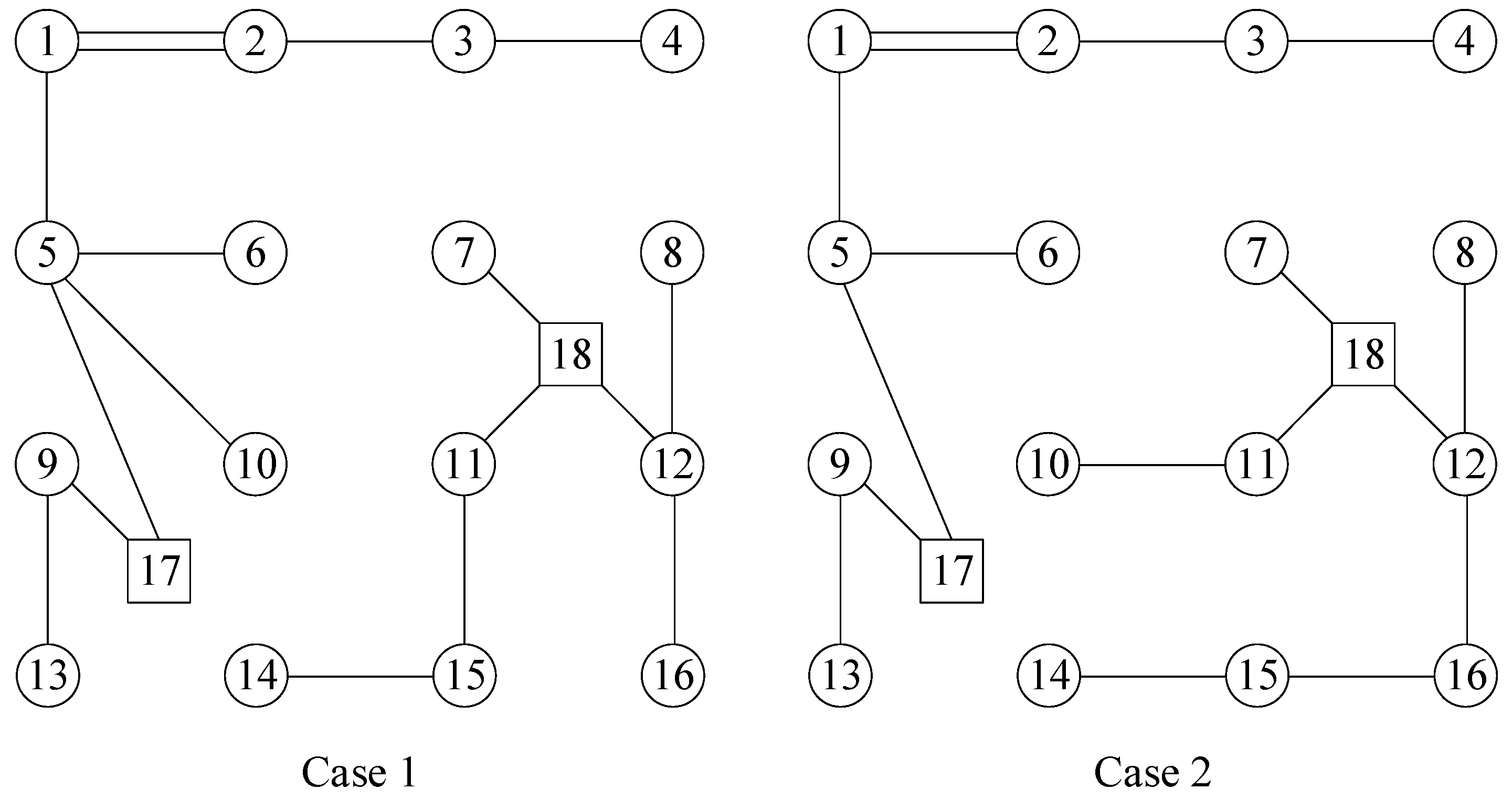
In this paper, an IES system is simulated with a network coupled with an 18-node distribution network and a 11-node low pressure natural gas network. The IES network topology is shown in Figure 7. The distribution network has 16 load nodes and 2 substation nodes, 24 planning lines of 20kV. Node 17 and node 18 are substation nodes, and the other nodes are electricity load nodes.

The natural gas network has 9 load nodes and 2 natural gas station nodes, 15 planning pipelines. Node 10 and node 11 nodes are natural gas station nodes, and the other nodes are gas load nodes.

The double solid line shown in the figure represents a fixed line or pipe. The single solid line represents the line or pipe to be replaced. The dashed line represents a new line or pipe to be added.

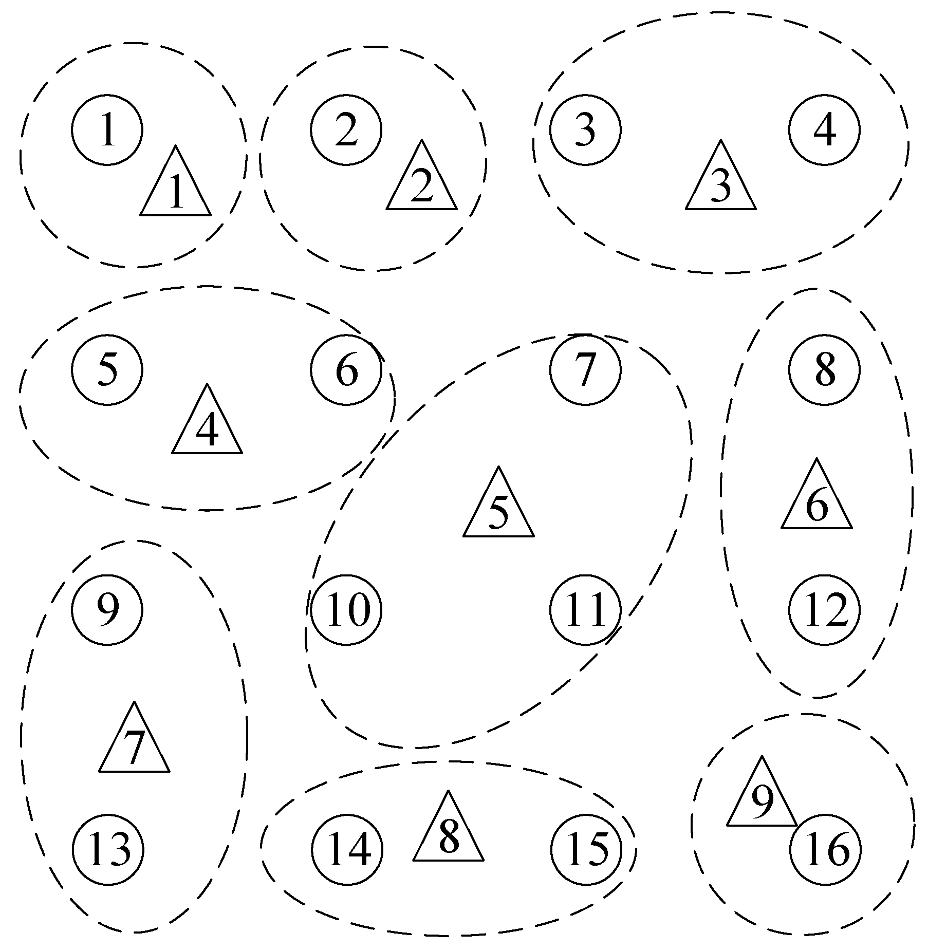
As shown in Figure 8, each natural gas load node covers natural gas, cold and heat loads in the adjacent electric load node. The natural gas node is set at one point in the coverage area, and the CCHP system is set at the node.

The two cases are listed as follows:

Case 1: CCHP is the couple of IES with electric air conditioner cooperated to supply electricity, gas, cold and heat load.

Case 2: SP cooperated with electric air conditioner to supply electricity, gas, cold and heat load.

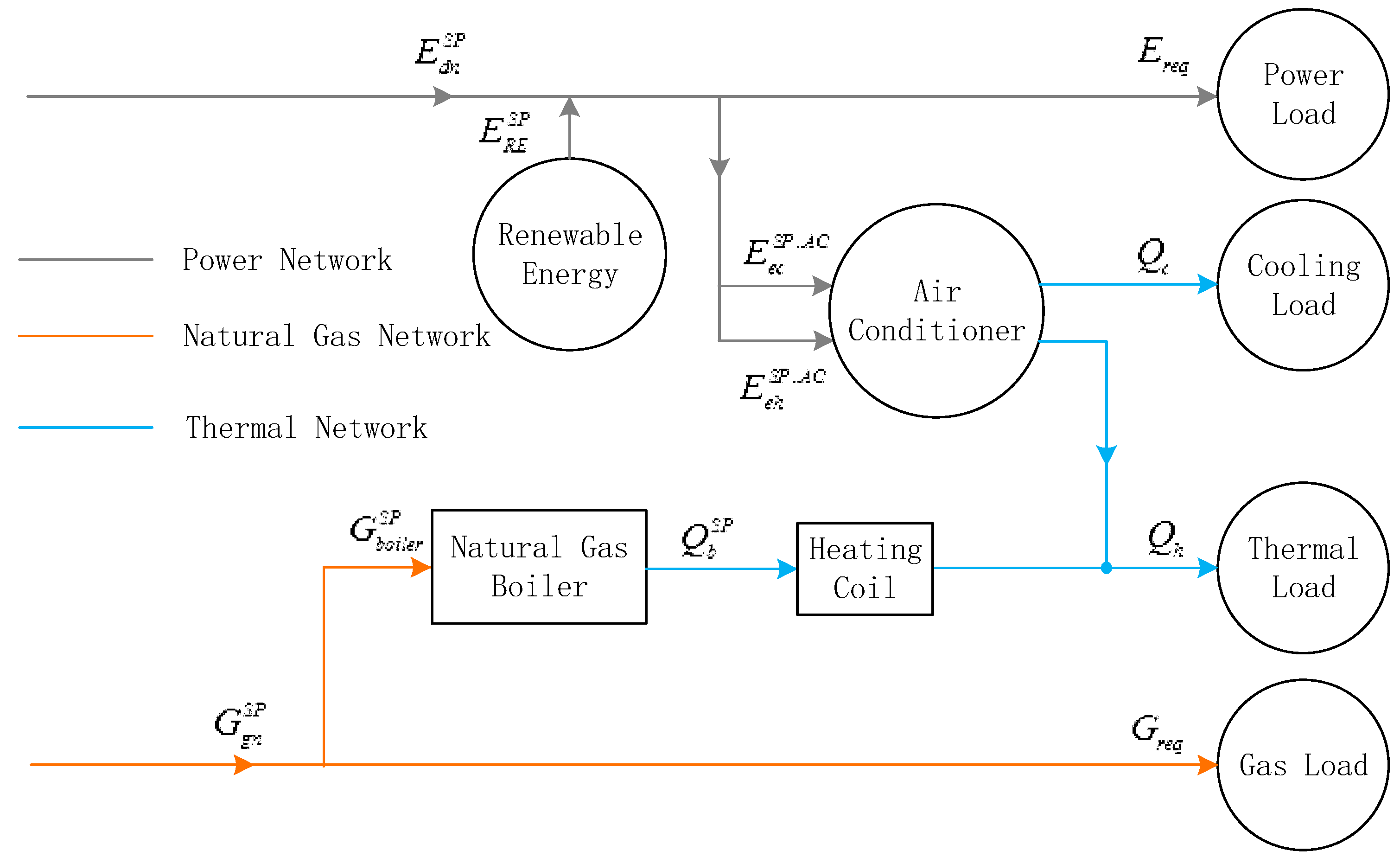
The physical programming model of SP, as shown in Figure 9, shows the connection and energy flow relation of gas boiler and heat exchanger, and how to cooperate with the electric air conditioner to output cold and heat load.

The CCHP and SP options are shown in

Table 1. Candidate options of CCHP and SP.

CCHP Options			SP Options
Gas Turbine Power/MW	Total Construction Cost/Thousand Dollars	Total Operation Cost/Thousand Dollars	Gas Boiler Power/MW	Total Construction Cost/Thousand Dollars	Total Operation Cost/Thousand Dollars
2.5	2500	250	4	2400	240
5.0	5000	500	8	4800	480
7.5	7500	750	12	7200	720

. The total construction cost and total operating cost in the CCHP selection scheme include the cost of gas turbine, gas boiler, heat recovery system and other equipment. The total construction cost and total operating cost in the SP selection scheme include the cost of gas-fired boilers, heat exchangers and other equipment. The three different capacity schemes of CCHP system and the three different capacity schemes of SP system are related to the characteristics of gas turbine and the gas boiler and their functions in their respective systems. Different capacity gas turbines and gas-fired boilers correspond to the different capacity schemes of the other equipment of their respective systems.

3.2. Case Results

The cost comparison of each case is shown in

Table 2. Cost comparison for cases.

Case	Case1	Case2
Total cost/thousand dollars	292,920	328,610
Construction cost of distribution network/thousand dollars	2470	3580
Operation cost of distribution network/thousand dollars	700	700
Construction cost of gas pipeline network/thousand dollars	6810	3550
Operation cost of gas pipeline network/thousand dollars	500	370
Construction cost of CCHP or SP/thousand dollars	233,90	161,20
Operation cost of CCHP or SP/thousand dollars	2580	810
Cost of electricity purchase/thousand dollars	152,580	272,310
Cost of gas purchase/thousand dollars	103,890	311,70

.

The time price curve of electricity load is derived from the official website of PJM company of the United States. The time-sharing price curve of natural gas comes from the official website of Henry trading center of the United States.

4. Discussion

4.1. Result Analysis

(1) Total cost analysis

Case1 < Case2

The total cost of CCHP system is lower than that of SP system, which mainly comes from the decline in the cost of purchasing electricity from the power grid.

(2) Cost analysis of distribution network

With CCHP coupling electric-gas system, gas turbine power generation can supply local electric load, which reduces transmission power of distribution network. Distribution network can choose distribution line model with lower maximum load flow and more flexible network frame construction. The two cases of third stage line planning results are shown in Figure 10.

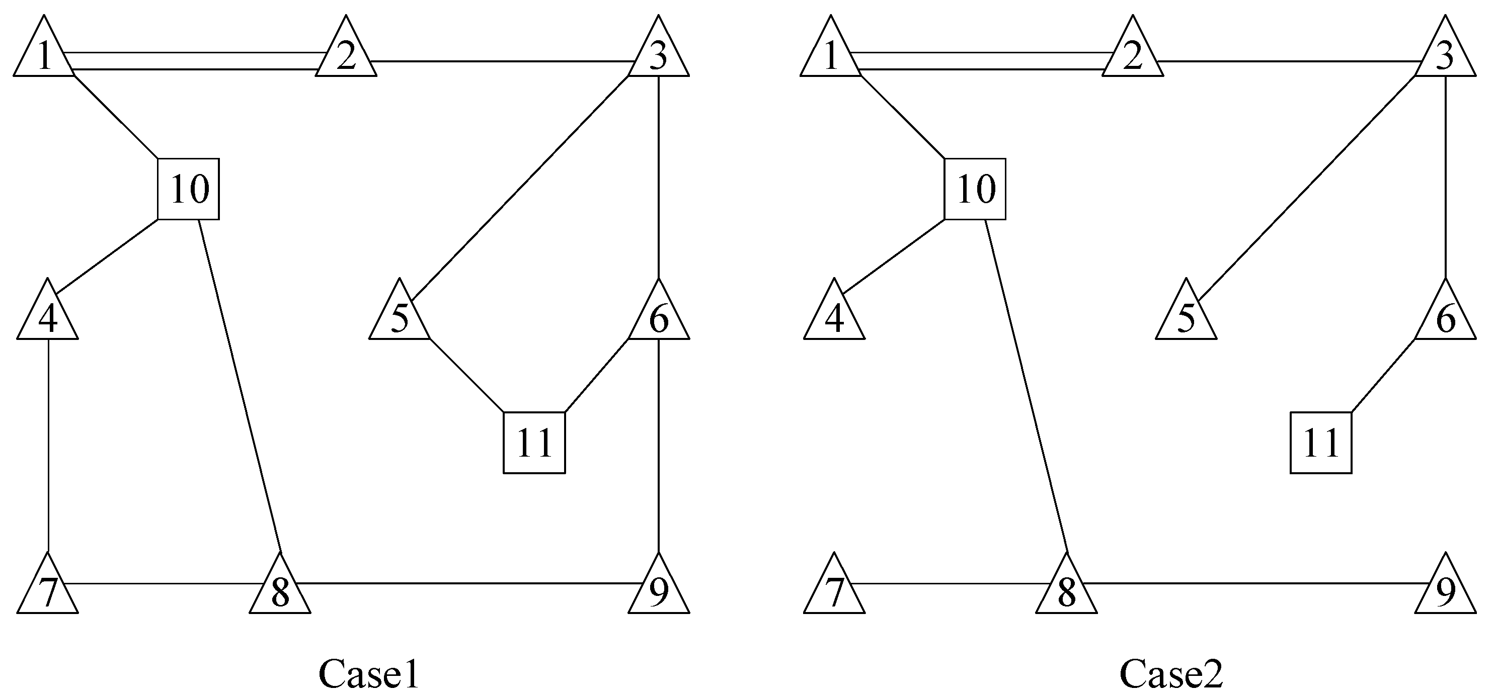
(3) Cost analysis of gas pipeline network

In addition to the same natural gas load supplied by the CCHP and SP systems, gas turbines and gas-fired boilers in CCHP also consume natural gas and supply electric, cold and heat loads. In SP, only gas-fired boilers consume natural gas and only supply heat load. Therefore, the natural gas flow of the Case1 is larger, and the selected gas pipeline price is also higher. The two cases of third stage pipeline planning results are shown in Figure 11.

(4) Cost of CCHP or SP

There are more internal devices in CCHP, and the construction operation cost under the same capacity is higher than that of SP. At the same time, it is considered that the electric air conditioner built by the user side can supply cold and heat load. Some nodes in the SP system do not have to build the gas boiler for heating. The CCHP system has the high efficiency of comprehensive energy use. compared with the electric air conditioner, the cost of cold and heat load in CCHP is low, so most of the nodes will build a combined cooling heating and power system. Thus, the construction and operation cost of the CCHP system will be higher than that of the SP system.

(5) Cost of purchasing electricity and natural gas

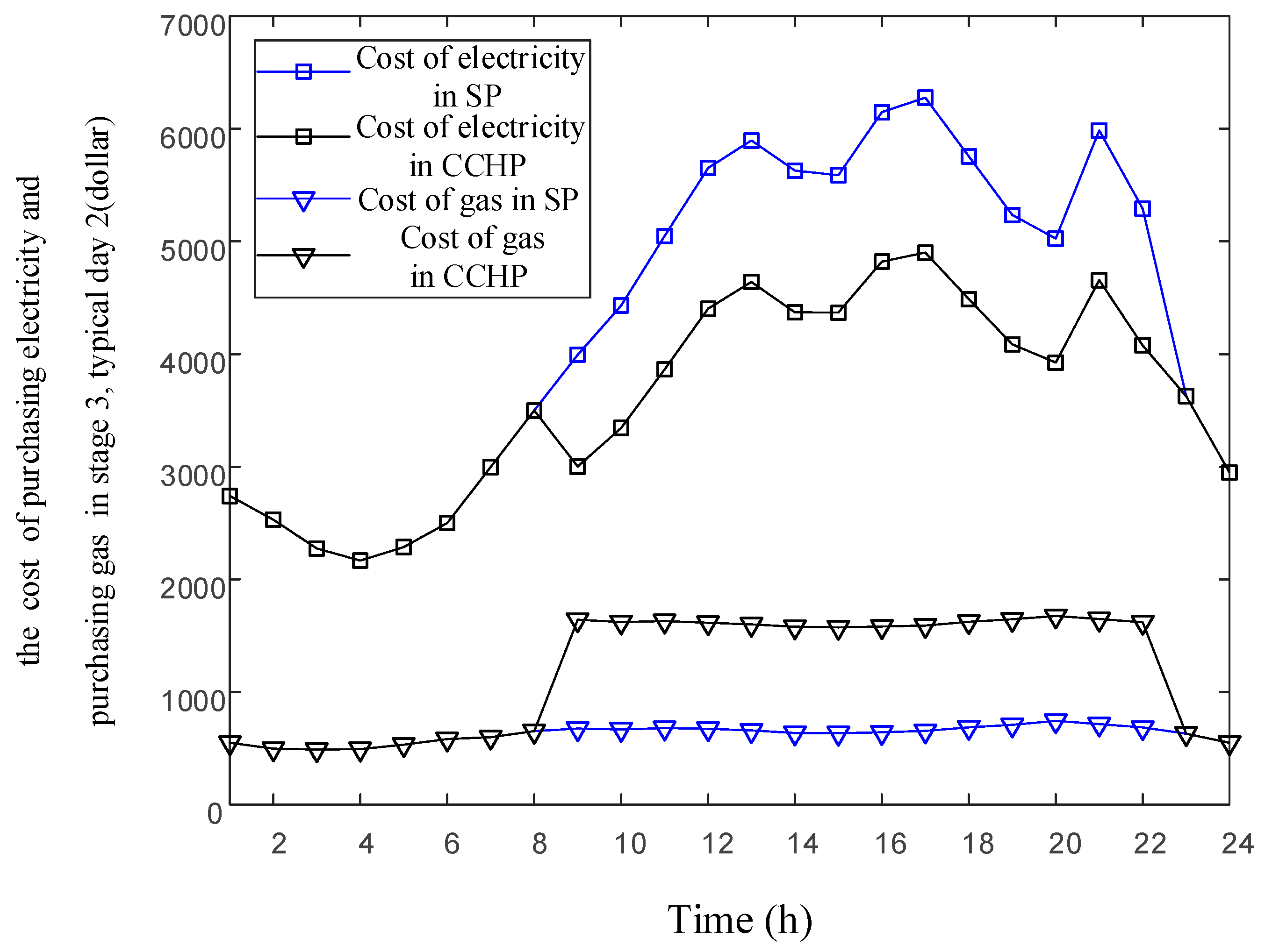
On the one hand, the gas turbine in CCHP can use waste heat to supply cold and heat load, on the other hand, the gas turbine generation can supply electricity load. Although more natural gas is used, the cost of gas purchase will be improved. The cost of electricity purchase will be greatly reduced, and the total cost will be reduced.

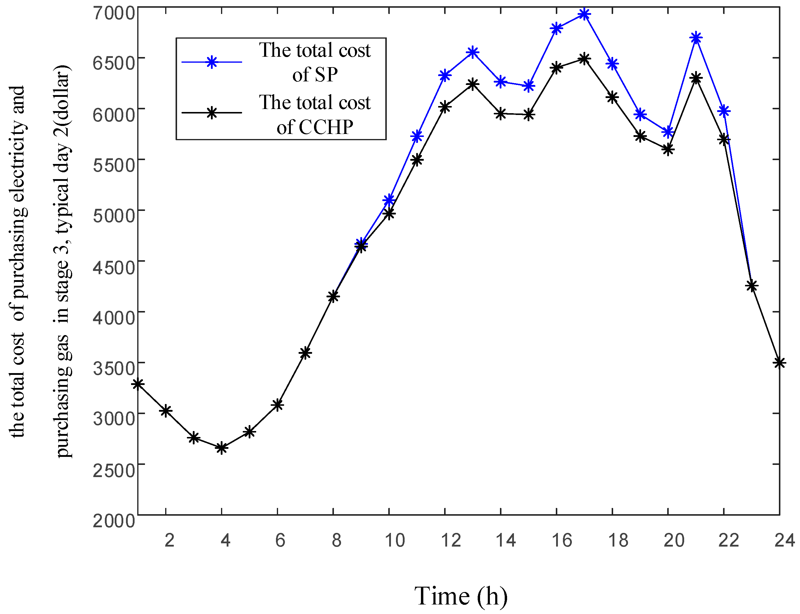
The cost of purchasing electricity from the power grid and the cost of purchasing gas from the natural gas network in stage 3, typical day 2 of the two cases are shown in Figure 12. The total cost of purchasing electricity and purchasing natural gas in stage 3, typical day 2 of the two cases is shown in Figure 13. From 23 h to 8 h, the cost of purchasing electricity and the cost of purchasing gas in Case1 and Case2 are the same, which indicates that the gas turbine and auxiliary boilers in the CCHP system are not working at this time, and the gas boilers in the SP system are not working. It shows that the electricity price is low, and the cold and heat load are provided by the electric air conditioner. From 9 h to 22 h, the cost of purchasing electricity in the SP system is greater than that of CCHP system and the cost of gas in the SP system is less than that of CCHP system. It indicates that the electricity price is higher, and the absorption chiller and the heat recovery device in the CCHP system begin to supply cool and heat load.

This paper does not give unnecessary details on the specific replacing and adding schemes of power lines and gas pipelines, the optimal location and capacity of CCHP.

From the above discussion, it can be concluded that the case without coupled CCHP reveals higher economic costs. Although the cost of electricity is lower, the cost of gas is higher. Therefore, the total investment cost is higher. Obviously, the planning with CCHP as coupled hub attains higher comprehensive use rate of energy and promotes energy conservation and environmental protection.

In view of too many parameters in the model, the computation speed is slow. Thus, we consider adopting the Benders decomposition algorithm to simplify the presented MILP into a two-level optimization framework including master and sub problems.

4.2. Impact Analysis of Price Factors

It is known from the previous section that the cost of purchasing electricity and gas are the most in the total cost of CCHP. Under the condition of constant electric, gas, cold and heat load, the electricity price, and natural gas price will affect the cost of purchasing electricity and the cost of purchasing gas. At the same time, because CCHP is the coupled hub, the relationship between the electricity price and the natural gas price will directly affect the relationship between the quantity of purchasing electricity and the quantity of purchasing gas.

For the specific typical day, the time price curve of electricity price and gas price will affect the quantity of purchasing electricity and gas. For any hour of the typical day, if the electricity price is higher and the gas price is lower, the price of the gas turbine generation will be low. If the price is lower than the purchasing electricity price, the gas turbine will generate. If the electricity price is lower and the gas price is higher, the price of gas turbine generation is higher. If the price is higher than the purchasing electricity price, the gas turbine will not generate.

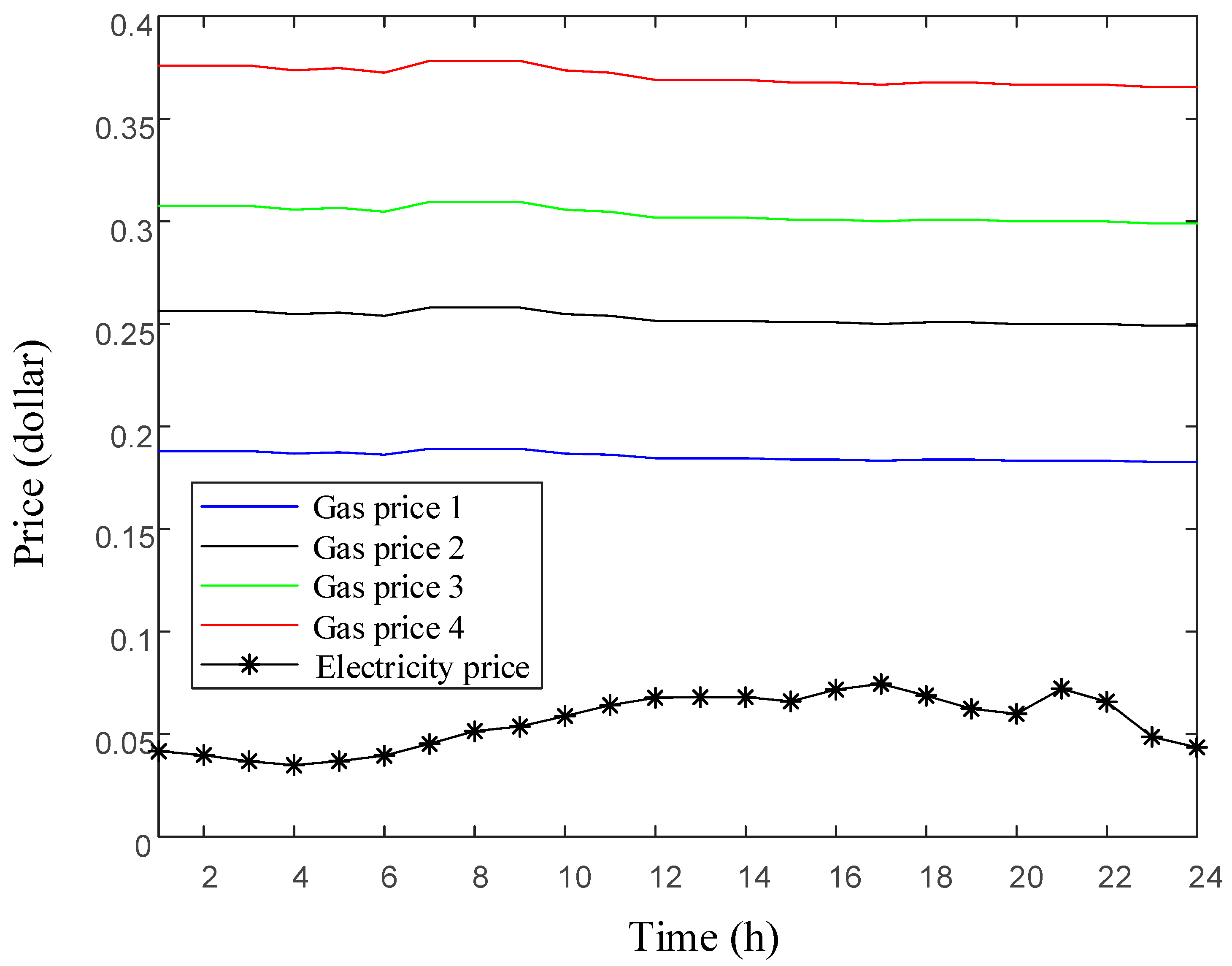
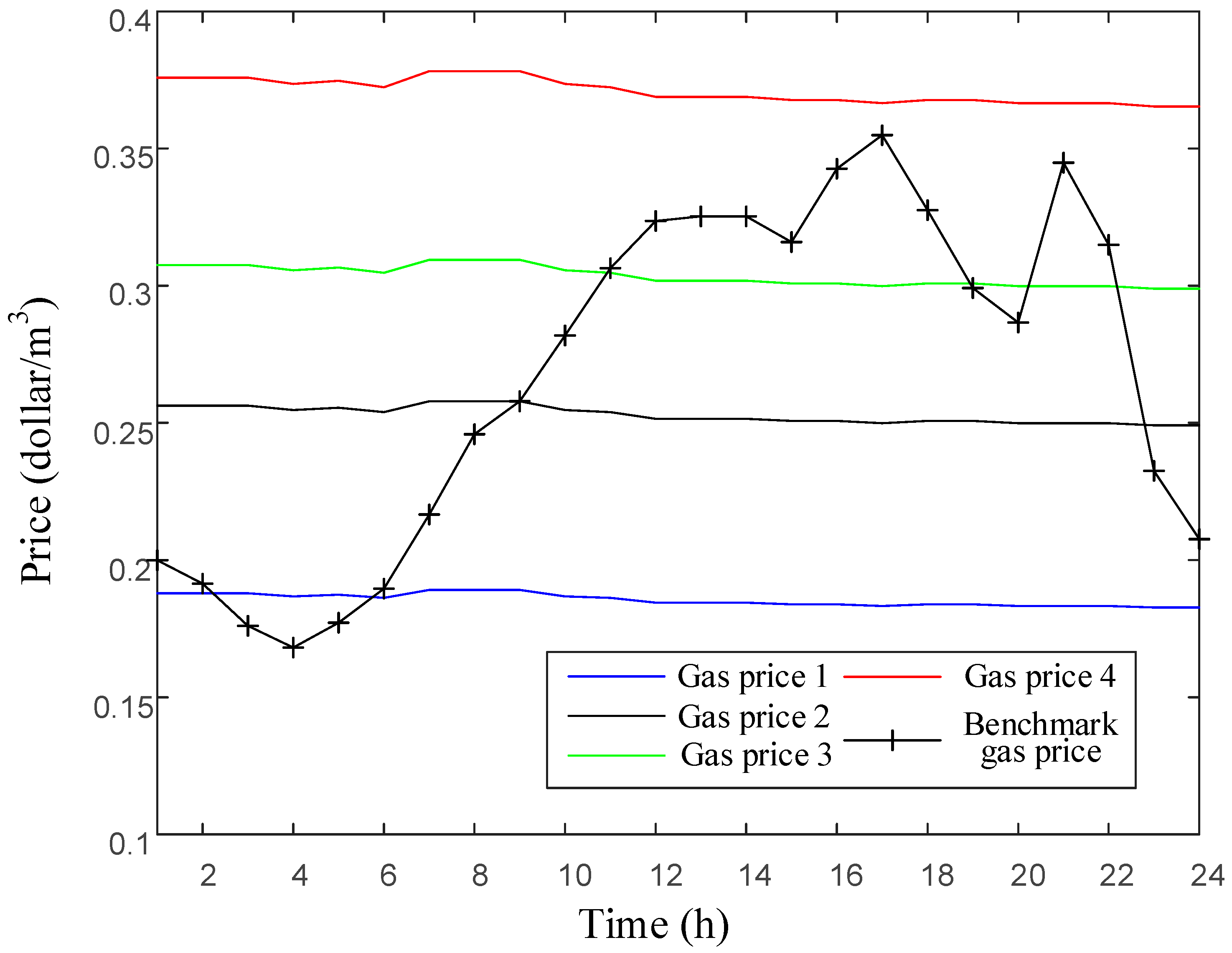
Different natural gas prices and fixed electricity price in the stage 3, typical day 2 are shown in Figure 14. The electricity price is the electricity price in the upper section case. The gas price 2 is the gas price in the upper section case. The gas price 1, the gas price 3, and the gas price 4 are 0.73 times, 1.2 times and 1.47 times of the gas price 2, respectively. The electricity price of 4 h is the low, and the electricity price of 17 h and 21 h is high. Compared with electricity price, the price of gas fluctuates less in the whole day.

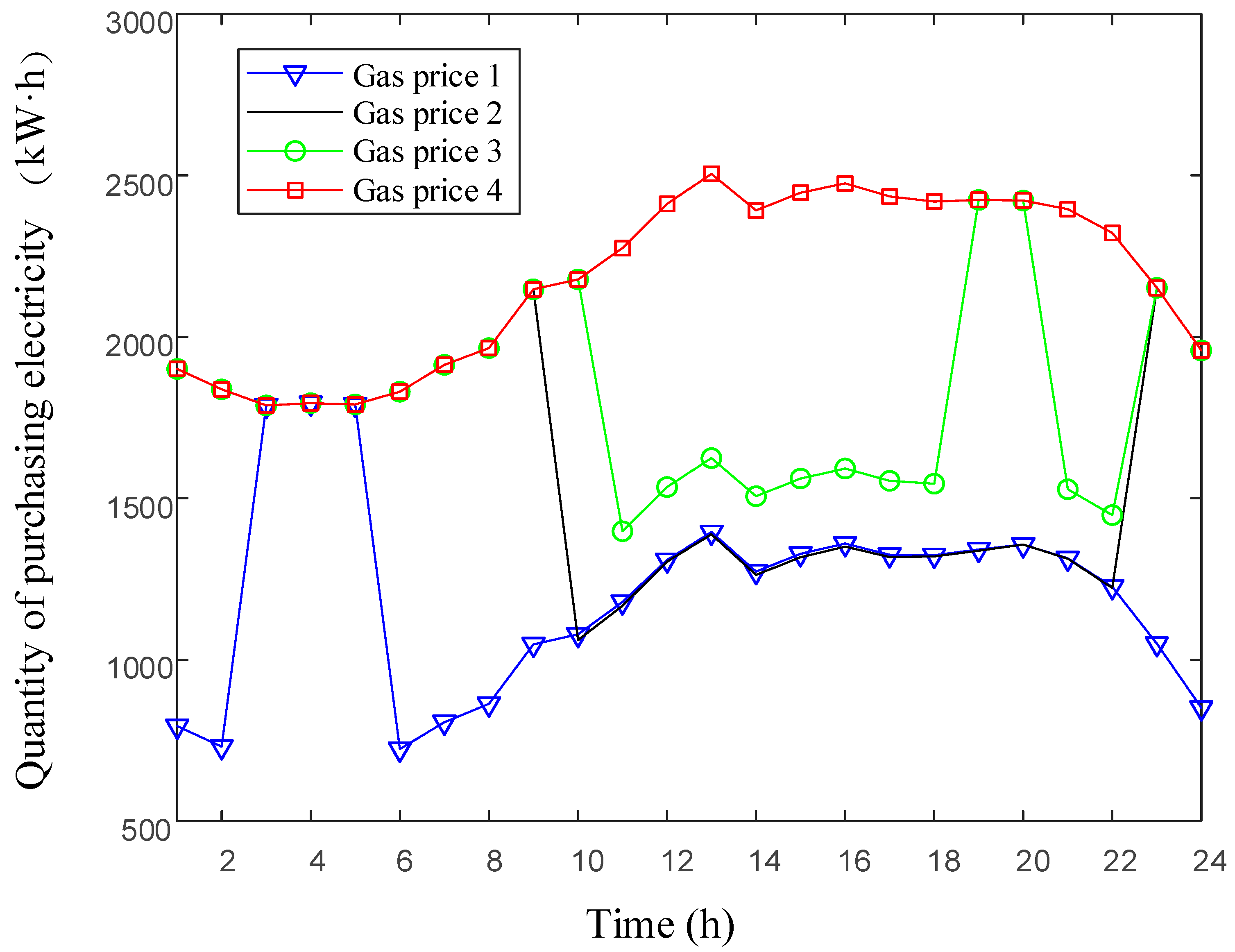
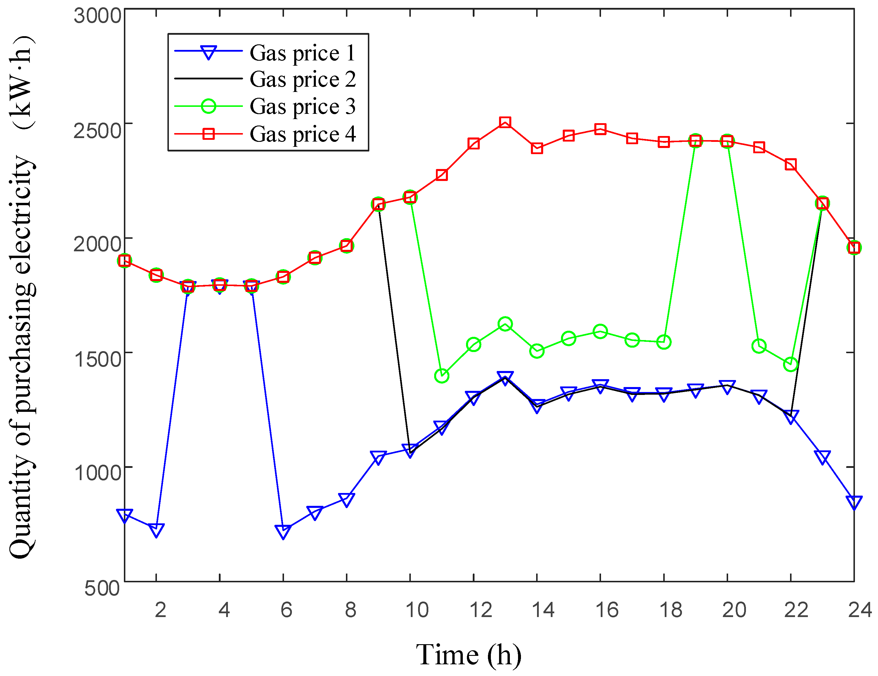
The quantity of purchasing electricity for different gas prices in stage 3, typical day 2 is shown in Figure 15. The quantity of purchasing gas for different gas prices in stage 3, typical day 2 is shown in Figure 16.

Different gas prices and benchmark gas price in stage 3, typical day 2 are shown in Figure 17. The benchmark natural gas price is the natural gas price that matches the given electricity price, which is, based on the electricity price at every moment, the price of the critical natural gas for the gas turbine to choose power generation at this time. When the actual gas price is higher than benchmark gas price, the gas turbine does not generate, and when the actual natural gas price is lower than the price, the gas turbine starts to generate.

From the gas price 1 curve and the benchmark natural gas price curve of Figure 17, the gas price 1 is higher than the benchmark natural gas price during 3 h to 5 h, indicating that the actual gas price is higher, and the gas turbine does not generate at this time. Therefore, the quantity of purchasing electricity of gas price 1 in Figure 15 is the largest, and the quantity of purchasing gas of gas price 1 in Figure 16 is the smallest. For other moments, gas price 1 is lower than the benchmark natural gas price, indicating that the actual gas price is lower and gas turbine generates at the time. Therefore, the quantity of purchasing electricity of gas price 1 in Figure 15 reaches the minimum, and the quantity of purchasing gas of gas price 1 in Figure 16 reaches the maximum. In addition to the fixed electricity load supplied by the gas turbine, all the other electricity loads come from the upper power grid. Thus, the quantity of purchasing electricity fluctuates with the electricity load curve.

From the gas price 2 curve and the benchmark natural gas price curve of Figure 17, the gas price 2 is lower than the benchmark natural gas price during 10 h to 22 h, indicating that the actual gas price is lower, and the gas turbine generates at this time. Therefore, the quantity of purchasing electricity of gas price 2 in Figure 15 reaches the minimum, and the quantity of purchasing gas of gas price 2 in Figure 16 reaches the maximum. For other moments, gas price 2 is higher than the benchmark natural gas price, indicating that the actual gas price is higher, and the gas turbine does not generate at this time. Therefore, the quantity of purchasing electricity of gas price 2 in Figure 15 reaches the maximum, and the quantity of purchasing gas of gas price 2 in Figure 16 reaches the minimum, which only meets the basic gas load.

From the gas price 3 curve and the benchmark natural gas price curve of Figure 17, the gas price 3 is lower than the benchmark natural gas price during 11 h to 18 h and 21 h to 22 h, indicating that the actual gas price is lower, and the gas turbine generates at this time. Therefore, the quantity of purchasing electricity of gas price 3 in Figure 15 reaches the minimum, and the quantity of purchasing gas of gas price 3 in Figure 16 reaches the maximum. However, the quantity of purchasing electricity is not the lowest, and the quantity of purchasing gas is not the highest. Because the benchmark gas price is only a measure of whether the gas turbine is generating. When the gas turbine chooses to generate, the proportion of the actual generation capacity to the rated power generation is related to the actual natural gas price. According to the simulation analysis, when the actual gas price is not higher than the gas price 2, the actual generation capacity reaches the rated power generation. When the actual gas price is higher than the gas price 2, the actual power generation is lower than the rated power generation, and the higher the actual natural gas price is, the lower the proportion of the actual power generation is. For other moments, gas price 3 is higher than the benchmark natural gas price, indicating that the actual gas price is higher, and the gas turbine does not generate at this time. Therefore, the quantity of purchasing electricity of gas price 3 in Figure 15 reaches the maximum, and the quantity of purchasing gas of gas price 3 in Figure 16 reaches the minimum.

From the gas price 4 curve and the benchmark natural gas price curve of Figure 17, the gas price 4 is higher than the benchmark natural gas price at any time, indicating that the gas turbine does not generate. Therefore, the quantity of purchasing electricity of gas price 4 in Figure 15 reaches the maximum, and the quantity of purchasing gas of gas price 4 in Figure 16 reaches the minimum.

5. Conclusions

In this paper, an optimal planning model of an electricity-gas IES based on coupled CCHP is proposed. The distribution lines expansion and construction scheme, gas pipelines expansion and construction scheme, CCHP construction and selection scheme are obtained through case analysis, which verifies the validity of the model.

The optimization model proposed in this paper is to consider how to plan and run IES rationally from the perspective of regional energy suppliers. In addition, the planning results bring many effective suggestions to regional energy suppliers on system planning and operation schedule. With the continuous deepening of the electric power system reform and the continuous development of IES, the role of regional energy suppliers is bound to appear. How to run IES rationally and efficiently will become a research focus in the future.

References

- U.S. Energy Information Administration, Monthly Energy Review. Available online: https://www.eia.gov/totalenergy/data/monthly/ (accessed on 15 June 2018).
- Liu, X.; Mancarella, P. Modelling, assessment and Sankey diagrams of integrated electricity-heat-gas networks in multi-vector district energy systems. Appl. Energy 2016, 167, 336–352. [Google Scholar] [CrossRef]
- Hibbard, P.J.; Schatzki, T. The interdependence of electricity and natural gas: Current factors and future prospects. Electr. J. 2012, 25, 6–17. [Google Scholar] [CrossRef]
- Quelhas, A.; Gil, E.; Mccalley, J.D.; Ryan, S.M. A Multiperiod generalized network flow model of the U.S. integrated energy system: Part I—Model description. IEEE Trans. Power Syst. 2007, 22, 829–836. [Google Scholar] [CrossRef]
- Chen, S.; Wei, Z.; Sun, G.; Cheung, K.W.; Sun, Y. Multi-linear probabilistic energy flow analysis of integrated electrical and natural-gas systems. IEEE Trans. Power Syst. 2017, 32, 1970–1979. [Google Scholar] [CrossRef]
- Wu, J.; Yan, J.; Jia, H.; Hatziargyriou, N.; Djilali, N.; Sun, H. Integrated Energy Systems. Appl. Energy 2016, 167, 155–157. [Google Scholar] [CrossRef]
- Shao, C.; Wang, X.; Shahidehpour, M.; Wang, X.; Wang, B. An MILP-Based optimal power flow in multicarrier energy systems. IEEE Trans. Sustain. Energy 2017, 8, 239–248. [Google Scholar] [CrossRef]
- Qu, K.; Yu, T.; Huang, L.; Yang, B.; Zhang, X. Decentralized optimal multi-energy flow of large-scale integrated energy systems in a carbon trading market. Energy 2018, 149, 779–791. [Google Scholar] [CrossRef]
- Martinez-Mares, A.; Fuerte-Esquivel, C.R. A Unified Gas and Power Flow Analysis in Natural Gas and Electricity Coupled Networks. IEEE Trans. Power Syst. 2012, 27, 2156–2166. [Google Scholar] [CrossRef]
- Geidl, M.; Andersson, G. Optimal Power Flow of Multiple Energy Carriers. IEEE Trans. Power Syst. 2007, 22, 145–155. [Google Scholar] [CrossRef] [Green Version]
- Moeini-Aghtaie, M.; Abbaspour, A.; Fotuhi-Firuzabad, M.; Hajipour, E. A decomposed solution to multiple-energy carriers optimal power flow. IEEE Trans. Power Syst. 2014, 29, 707–716. [Google Scholar] [CrossRef]
- Lei, Y.; Hou, K.; Wang, Y.; Jia, H.; Zhang, P.; Mu, Y.; Jin, X.; Sui, B. A new reliability assessment approach for integrated energy systems: Using hierarchical decoupling optimization framework and impact-increment based state enumeration method. Appl. Energy 2018, 210, 1237–1250. [Google Scholar] [CrossRef]
- Clegg, S.; Mancarella, P. Integrated Electrical and Gas Network Flexibility Assessment in Low-Carbon Multi-Energy Systems. IEEE Trans. Sustain. Energy 2016, 7, 718–731. [Google Scholar] [CrossRef]
- Clegg, S.; Mancarella, P. Integrated Electricity-Heat-Gas Modelling and Assessment, with Applications to the Great Britain System. Part I: High-Resolution Spatial and Temporal Heat Demand Modelling. Energy 2018. [Google Scholar] [CrossRef]
- Chen, X.; Mcelroy, M.B.; Kang, C. Integrated Energy Systems for Higher Wind Penetration in China: Formulation, Implementation and Impacts. IEEE Trans. Power Syst. 2018, 33, 1309–1319. [Google Scholar] [CrossRef]
- Shao, C.; Shahidehpour, M.; Wang, X.; Wang, X.; Wang, B. Integrated Planning of Electricity and Natural Gas Transportation Systems for Enhancing the Power Grid Resilience. IEEE Trans. Power Syst. 2017, 32, 4418–4429. [Google Scholar] [CrossRef]
- Wu, L.; He, C.; Dai, C.; Liu, T. Robust Network Hardening Strategy for Enhancing Resilience of Integrated Electricity and Natural Gas Distribution Systems Against Natural Disasters. IEEE Trans. Power Syst. 2018, 33, 5787–5798. [Google Scholar]
- Li, G.; Bie, Z.; Kou, Y.; Jiang, J.; Bettinelli, M. Reliability evaluation of integrated energy systems based on smart agent communication. Appl. Energy 2016, 167, 397–406. [Google Scholar] [CrossRef]
- Pambour, K.A.; Erdener, B.C.; Bolado-Lavin, R.; Dijkema, G.P. SAInt—A novel quasi-dynamic model for assessing security of supply in coupled gas and electricity transmission networks. Appl. Energy 2017, 203, 829–857. [Google Scholar] [CrossRef]
- Saldarriaga, C.A.; Hincapié, R.A.; Salazar, H. A Holistic Approach for Planning Natural Gas and Electricity Distribution Networks. IEEE Trans. Power Syst. 2013, 28, 4052–4063. [Google Scholar] [CrossRef]
- Odetayo, B.; Maccormack, J.; Rosehart, W.D.; Zareipour, H. A sequential planning approach for Distributed generation and natural gas networks. Energy 2017, 127, 428–437. [Google Scholar] [CrossRef]
- Zhao, B.; Conejo, A.J.; Sioshansi, R. Coordinated Expansion Planning of Natural Gas and Electric Power Systems. IEEE Trans. Power Syst. 2018, 33, 3064–3075. [Google Scholar] [CrossRef]
- Zhang, X.; Che, L.; Shahidehpour, M.; Ahmed, A.; Abdullah, A. Electricity-Natural Gas Operation Planning with Hourly Demand Response for Deployment of Flexible Ramp. IEEE Trans. Sustain. Energy 2016, 7, 996–1004. [Google Scholar] [CrossRef]
- Ceseña, E.A.M.; Capuder, T.; Mancarella, P. Flexible Distributed Multienergy Generation System Expansion Planning Under Uncertainty. IEEE Trans. Smart Grid 2015, 7, 348–357. [Google Scholar] [CrossRef]
- He, C.; Wu, L.; Liu, T.; Bei, Z. Robust Co-optimization Planning of Interdependent Electricity and Natural Gas Systems with a Joint N-1 and Probabilistic Reliability Criterion. IEEE Trans. Power Syst. 2017, 33, 2140–2154. [Google Scholar] [CrossRef]
- Unsihuay-Vila, C.; Marangon-Lima, J.W.; de Souza, A.Z.; Perez-Arriaga, I.J.; Balestrassi, P.P. A Model to Long-Term, Multiarea, Multistage, and Integrated Expansion Planning of Electricity and Natural Gas Systems. IEEE Trans. Power Syst. 2010, 25, 1154–1168. [Google Scholar] [CrossRef]
- Qiu, J.; Dong, Z.Y.; Zhao, J.H.; Xu, Y.; Zheng, Y.; Li, C.; Wong, K.P. Multi-Stage Flexible Expansion Co-Planning Under Uncertainties in a Combined Electricity and Gas Market. IEEE Trans. Power Syst. 2015, 30, 2119–2129. [Google Scholar] [CrossRef]
- Sadeghian, H.R.; Ardehali, M.M. A novel approach for optimal economic dispatch scheduling of integrated combined heat and power systems for maximum economic profit and minimum environmental emissions based on Benders decomposition. Energy 2016, 102, 10–23. [Google Scholar] [CrossRef]
- Jiang, Y.; Xu, J.; Sun, Y.; Wei, C.; Wang, J.; Liao, S. Coordinated operation of gas-electricity integrated distribution system with multi-CCHP and distributed renewable energy sources. Appl. Energy 2018, 211, 237–248. [Google Scholar] [CrossRef]
- Pazouki, S.; Mohsenzadeh, A.; Ardalan, S.; Haghifam, M.R. Optimal place, size, and operation of combined heat and power in multi carrier energy networks considering network reliability, power loss, and voltage profile. IET Gen. Transm. Distrib. 2016, 10, 1615–1621. [Google Scholar] [CrossRef]
- Bao, Z.; Zhou, Q.; Yang, Z.; Yang, Q.; Xu, L.; Wu, T. A Multi Energy-Type Coordinated Microgrid Scheduling Solution—Part I: Model and Methodology. IEEE Trans. Power Syst. 2015, 30, 2257–2266. [Google Scholar] [CrossRef]
- Bao, Z.; Zhou, Q.; Yang, Z.; Xu, L.; Wu, T. A Multi Time-Scale and Multi Energy-Type Coordinated Microgrid Scheduling Solution—Part II: Optimization Algorithm and Case Studies. IEEE Trans. Power Syst. 2015, 30, 2267–2277. [Google Scholar] [CrossRef]
- Li, G.; Zhang, R.; Jiang, T.; Chen, H.; Bai, L.; Cui, H. Optimal dispatch strategy for integrated energy systems with CCHP and wind power. Appl. Energy 2016, 192, 408–419. [Google Scholar] [CrossRef]
- Fang, F.; Wang, Q.H.; Shi, Y. A Novel Optimal Operational Strategy for the CCHP System Based on Two Operating Modes. IEEE Trans. Power Syst. 2012, 27, 1032–1041. [Google Scholar] [CrossRef]
- Wu, D.W.; Wang, R.Z. Combined cooling, heating and power: A review. Prog. Energy Combust. Sci. 2006, 32, 459–495. [Google Scholar] [CrossRef]
- Wall, D.L.; Thompson, G.L.; Northcote-Green, J.E.D. An Optimization Model for Planning Radial Distribution Networks. IEEE Trans. Power Appar. Syst. 1979, PAS-98, 1061–1068. [Google Scholar] [CrossRef]
- Shen, X.; Shahidehpour, M.; Zhu, S.; Han, Y.; Zheng, J. Multi-stage Planning of Active Distribution Networks Considering the Co-optimization of Operation Strategies. IEEE Trans. Smart Grid 2018, 9, 1425–1433. [Google Scholar] [CrossRef]
- Chen, J.; Lv, L.; Xu, X. The distribution network reconfiguration based on spanning tree. In Proceedings of the 2nd International Conference on Information Science and Engineering, Hangzhou, China, 4–6 December 2010; pp. 7017–7020. [Google Scholar]
Figure 1.
IES Physical planning model.
Figure 2.
CCHP Physical planning model.
Figure 3.
IES optimization planning model.
Figure 4.
Linearized schematic diagram of relationship between natural gas flow and pressure.
Figure 5.
Output curve of wind turbine.
Figure 6.
Output curve of photovoltaic.
Figure 7.
Topology of IES network.
Figure 8.
The corresponding graph of natural gas load node and electric load node.
Figure 9.
SP physical planning model.
Figure 10.
Power lines planning topologies of different cases in stage 3.
Figure 11.
Gas pipelines planning topologies of different cases in stage 3.
Figure 12.
Cost curves of purchasing electricity and purchasing gas for different cases in stage 3, typical day 2.
Figure 13.
Total cost curves of purchasing electricity and purchasing gas for different cases in stage 3, typical day 2.
Figure 14.
Different gas prices and electricity price in stage 3, typical day 2.
Figure 15.
Quantity of purchasing electricity for different gas prices in stage 3, typical day 2.
Figure 16.
Quantity of purchasing gas for different gas prices in stage 3, typical day 2.