Simulation and Exergy Analysis of Energy Conversion Processes Using a Free and Open-Source Framework—Python-Based Object-Oriented Programming for Gas- and Steam Turbine Cycles

Abstract

State-of-the-art thermodynamic simulation of energy conversion processes requires proprietary software. This article is an attempt to refute this statement. Based on object-oriented programming a simulation and exergy analysis of a combined cycle gas turbine is carried out in a free and open-source framework. Relevant basics of a thermodynamic analysis with exergy-based methods and necessary fluid property models are explained. Thermodynamic models describe the component groups of a combined heat and power system. The procedure to transform a physical model into a Python-based simulation program is shown. The article contains a solving algorithm for a precise gas turbine model with sophisticated equations of state. As an example, a system analysis of a combined cycle gas turbine with district heating is presented. Herein, the gas turbine model is validated based on literature data. The exergy analysis identifies the thermodynamic inefficiencies. The results are graphically presented in a Grassmann chart. With a sensitivity analysis a thermodynamic optimization of the district heating system is discussed. Using the exergy destruction rate in heating condensers or the overall efficiency as the objective function yields to different results.

1. Introduction

We prefer lectures and exercises in which students may bring their own device, also known as bring your own device (BYOD) policy, cp. Reference [1] pp. 36–37, and are able to use several software for the simulation and optimization of energy conversion processes. A lot of professional software contributers have an academical license program. Unfortunately, these volume licenses are becoming more expensive for colleges or its use is restricted to computers in departments only. For example F-Chart Software announced a renewal agreement for the Engineering Equation Solver (EES) academic license in May 2017. In consequence, the simulation tool EES “may not be installed on personal computers. It may only be installed on computers owned or controlled by the adopting department.” [2] Instead of using an application virtualization we decided to run simple plots, parameter studies or elementary process models using Python. However, the question is immediately raised as to whether it is also possible to run a more complex simulation like a state-of-the-art combined cycle using a more precise gas turbine model and sophisticated equations of state in a complete open-source framework.

For fundamental publications on gas turbine technology we refer to the books of the following authors: Bathie [3] presents the fundamentals of a gas turbine system including the components. Giampaolos’ [4] gas turbine handbook faces principles and practice by confronting the theory with questions such as gas turbine control, inlet and exhaust treatment or detectable problems. Traupel [5,6] extensively discusses the thermodynamics of turbomachinery, while Lefebvre and Ballal [7] focus on gas turbine combustion. Lechner and Seume [8] especially discuss stationary gas turbines and Kehlhofer et al. [9] in particular combined-cycle gas and steam turbine power plants. In the field of advanced gas turbine cycles, Horlock [10] gives a comprehensive overview.

Due to the numerous publications on current and future developments regarding gas turbines (GT) and combined cycle gas turbines (CCGT), some reviews are principally mentioned here. Poullikkas [11] describes and compares current and future sustainable gas turbine technologies. González-Salazar [12] presents a technical analysis of carbon dioxide capture technologies for gas turbine power generation based on a literature review. Ibrahim et al. [13] perform a literature review in the field of the optimum performance of a combined cycle power plant, carry out a parametric analysis, and present simulation models to improve the efficiency of such power plants. Due to the expected higher share of fluctuating renewable energy sources in the future, González-Salazar et al. [14] review the operational flexibility of gas- and coal-fired power plants. The authors collect current and expected future values describing the flexibility, e.g., the number of starts, start time, ramp-rate or minimum downtime. With a closed-cycle or externally fired gas turbine other energy sources than natural gas such as solid or liquid fossil fuels, concentrated solar power, nuclear, biomass, and waste heat can be used. Olumayegun et al. [15] present an overview of the historical development and fundamental aspects of these systems. Alternative heat sources, working fluids, heat exchangers, and process designs are introduced by the authors. Al-attab and Zainal [16] also review the externally-fired gas turbine technology. Their focus is on the gas turbine itself and the different high-temperature heat-exchanger materials and designs. In a low-carbon future, hydrogen blends and syngas represent alternative fuels to natural gas. Taamallah et al. [17] review the progress of gas turbine combustion for hydrogen-rich synthetic gas (syngas) mixtures. The technology of flameless combustion enables the reduction of pollutant emissions without influence on the efficiency of the gas turbine system. Rather, homogeneous temperature distribution is achieved as well as noise and thermal stress are reduced. Khidr et al. [18] and Xing et al. [19] review this approach.

A further increase of the efficiency of gas turbine systems is strongly connected with the thermodynamics of combustion. Recent progress in the field of constant volume combustion is expected by using shockless explosion combustion. Bobusch et al. [20] stated that the disadvantages of the pulsed detonation combustion, “such as sharp pressure transitions, entropy generation due to shock waves, and exergy losses due to kinetic energy”, do not occur when using shockless explosion combustion. Berndt and Klein [21] document recent findings regarding the modeling of the kinetics and Rähse et al. [22] regarding the gas dynamic simulation.

The procedures of analyses using exergy-based methods are described in the textbooks of Szargut [23], Kotas [24], Fratzscher et al. [25], and Bejan et al. [26]. There are a large number of system analyses using these methods. Kumar [27] and Kauschik et al. [28] collect the current contributions with a focus on thermal power plants in comprehensive reviews. Ibrahim et al. [29] only consider this for combined cycle power plants. Nowadays, the advanced exergy-based analyses are being further developed. This approach is useful for a better understanding of the avoidable inefficiencies, see References [30,31], and of the thermodynamic interactions between components of a system, see References [32,33,34]. Penkuhn and Tsatsaronis [35] discuss the calculation of endogenous and exogenous exergy destruction.

Several authors carry out analyses of detailed gas turbine systems using exergy-based methods and commercial software. Blumberg et al. [36] carry out an exergoeconomic evaluation of state-of-the-art CCGT. The software Ebsilon Professional is used for the simulation of the process. The gas turbine system is modeled as a simple cycle without consideration of cooling air flows. Sorgenfrei and Tsatsaronis [37] describe the exergy-based evaluation of gas turbine systems. The detailed model of the process considers cooling and sealing air flows as well as excess air. Natural gas and syngas are possible fuels. The process is modeled using the software Aspen Plus. 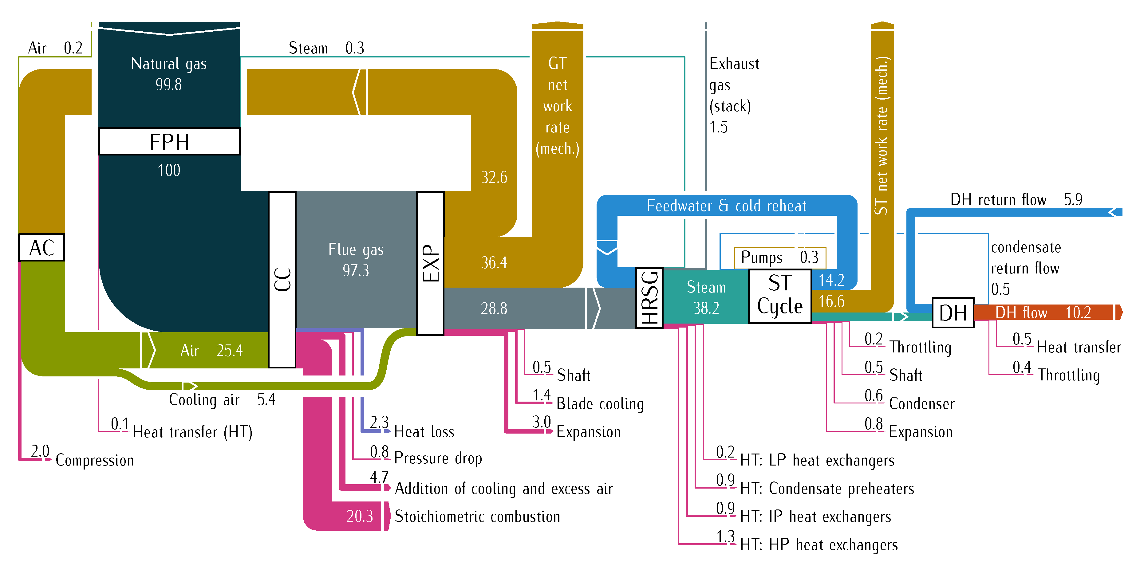Grassmann diagrams, see Reference [38], visualize the exergy destruction based on compression, stoichiometric combustion, addition of excess air, convective cooling, pressure drop, expansion, mixing at different pressures, temperatures and compositions, heat loss, transport of shaft work as well as conversion of mechanical into electrical energy.

Giglmayr [39] lists and discusses commercial software tools for steady state and dynamic simulation in the field of energy and process engineering. As mentioned, we would like to use a complete open-source framework for the thermodynamic simulation of energy conversion processes. In recent years, several developments were published. The Cantera framework, see Reference [40], which can be used from Python represents an open-source tool in the field of thermodynamics with a focus on reaction kinetics. Unfortunately, multiparameter equations of state for a wide range of fluids are not implemented. For properties of substances used in thermal power plants, Bell et al. [41] present an open-source framework called CoolProp which is based on multiparameter equations of state. This library is used by the applications DWSIM, see Reference [42], and ThermoCycle, see Reference [43]. DWSIM is an independently executable software useful for the simulation of chemical processes. Typical unit operations of process engineering such as reactors, columns, pumps, compressors, mixers, heat exchangers, etc., are implemented in the program. Furthermore, thermodynamic models of several equations of state for the properties of substances as well as a binary-mixture equilibrium-data regression can be used in simulations. ThermoCycle is a library within the Modelica modeling environment. Quoilin et al. [43] argue that the application was developed primarily for the simulation of thermal power plants. The focus is on systems with lower rated capacity and in particular on systems with organic working fluids. To avoid possible limitations of the mentioned applications, we decided to develop an open-source framework in Python using the library CoolProp to perform a simulation and exergy analysis of a combined cycle gas turbine.

The paper consists of the following five sections. Section 2 describes the methodology of thermodynamic modeling, including basics, exergy analysis, and models for fluid properties. Furthermore, it outlines the main component groups from a thermodynamic point of view. The methodology of programming, simulation, and calculation is summarized in Section 3. As an example of the approach shown in this paper, Section 4 consists of a description and depiction of a combined cycle gas turbine power plant as well as assumptions and given parameters. Section 5 reports the results of the validation, the exergy analysis as well as a sensitivity analysis. Conclusions are given in Section 6.

2. Thermodynamic Modeling

A combined cycle gas turbine is under investigation from a thermodynamic point of view. This chapter summarizes fundamental assumptions, the basics for the thermodynamic and exergy-based analysis as well as models for the fluid properties. Additionally, the system is described along its three main component groups, namely the gas turbine, the heat recovery steam generator (HRSG) together with the steam turbines, and the district heating system.

2.1. Basics

The model is used for a design case simulation, to calculate full-load operation at steady state conditions. As a result of the simulation, heat transfer surfaces are known. Therefore a further improvement of the model for the calculation of part load operations is possible. For all components of the systems we assume that:

• Changes in kinetic and potential energies and exergies are negligible.
• Heat losses over the surface of components are neglected, except for combustion chambers.
• Pressure drops are possible in all components, except mixers and splitters.

The process consists of a given number of components k and states j. Every state represents a stream of matter $\dot{H}$, mechanical or electrical power $\dot{W}$, or a heat rate $\dot{Q}$. A component is characterized by functions that could affect the states. For all components the balances of mass, energy, and exergy are given. In these i represents streams at the inlet, e streams at the outlet of a component, and r heat rates over the surface at temperature $T_r$.

$$\sum _i{\dot{m}}_{\mathrm{in},i}=\sum _e{\dot{m}}_{\mathrm{out},e}$$

(1)

$$0=\sum _r{\dot{Q}}_r+\dot{W}+\sum _i{\left(\dot{m}h\right)}_{\mathrm{in},i}-\sum _e{\left(\dot{m}h\right)}_{\mathrm{out},e}$$

(2)

$$0=\sum _r\underset{{\dot{E}}_{\mathrm{q},r}}{\underbrace{\left(1-\frac{T_0}{T_r}\right){\dot{Q}}_r}}+\dot{W}+\sum _i{\dot{E}}_{\mathrm{in},i}-\sum _e{\dot{E}}_{\mathrm{out},e}-{\dot{E}}_{\mathrm{D},k}$$

(3)

In addition to the parameters of the environment state, the absolute pressures of all states are given parameters. As such, they either have to be set explicitly or defined implicitly with pressure drops over the components. Parameters related to the function of a component, for example isentropic efficiencies or heat transfer coefficients, are usually given. The same holds for critical design data which includes, among others, the gas turbine inlet temperature or live and reheat steam temperatures.

2.2. Exergy Analysis

Since an energy analysis does not reveal the real inefficiencies in a process, an exergy analysis based on the simulation results for each state is included in the program. To carry out the analysis, it is necessary to define the exergetic fuel and product of the total process and the examined components. The exergetic loss rate is assigned to the total process. Equation (3) becomes then

$${\dot{E}}_{\mathrm{F},\mathrm{tot}}={\dot{E}}_{\mathrm{P},\mathrm{tot}}+{\dot{E}}_{\mathrm{D},\mathrm{tot}}+{\dot{E}}_{\mathrm{L},\mathrm{tot}}$$

(4)

for the total process and

$${\dot{E}}_{\mathrm{F},k}={\dot{E}}_{\mathrm{P},k}+{\dot{E}}_{\mathrm{D},k}$$

(5)

for a component. For the definition of fuel and product of the components we refer to References [44,45]. For a combined cycle heat and power system, the exergetic product is the sum of the net work rate and the total exergy rate of the heat transfered to the district heating system. The natural gas which enters the gas turbine represents the exergetic fuel. The exergetic efficiency of the total process can be defined.

$${\epsilon }_{\mathrm{chp}}=\frac{{\dot{W}}_{\mathrm{net}}+{\dot{E}}_{\mathrm{q},\mathrm{DH}}}{{\dot{m}}_{\mathrm{fuel}}·e_{\mathrm{fuel}}^{\mathrm{CH}}}$$

(6)

Furthermore, the exergy analysis is used to evaluate the exergetic efficiency of the components,

$${\epsilon }_k=\frac{{\dot{E}}_{\mathrm{P},k}}{{\dot{E}}_{\mathrm{F},k}}$$

(7)

the share of the total fuel exergy ${\dot{E}}_{\mathrm{F},\mathrm{tot}}$ destroyed in each component

$$y_{\mathrm{D},k}=\frac{{\dot{E}}_{\mathrm{D},k}}{{\dot{E}}_{\mathrm{F},\mathrm{tot}}}$$

(8)

and fuel exergy lost by heat or matter transfers to the environment.

$$y_{{}_{\mathrm{L}}}=\frac{{\dot{E}}_{\mathrm{L}}}{{\dot{E}}_{\mathrm{F},\mathrm{tot}}}$$

(9)

It is important to notice that the condenser is regarded as a dissipative component because the remaining steam exergy after the turbine is discarded by heat transfer to the cooling water.

2.3. Fluid Properties

The streams of matter are modeled using different equations of state. While the use of the IAPWS (International Association for the Properties of Water and Steam) 1995 formulation for water, see Reference [46], is standard practice, the gaseous mixtures included in the model, namely air, natural gas and flue gases, are represented by the GERG (Groupe Européen de Recherches Gaziéres) 2008 formulation, see Reference [47]. This equation of state is applicable to arbitrary compositions of 21 chemical components typically found in natural gas and its (stochiometric) combustion products. Its great advantage is the representation of real gas behavior compared to most equations of state that emanate from the assumption of ideal gas behavior using reference states. Instead, the GERG equations are based on the free enthalpy of each component and also include the excess enthalpy of every possible component pair in the given mixture.

2.4. Gas Turbine Model

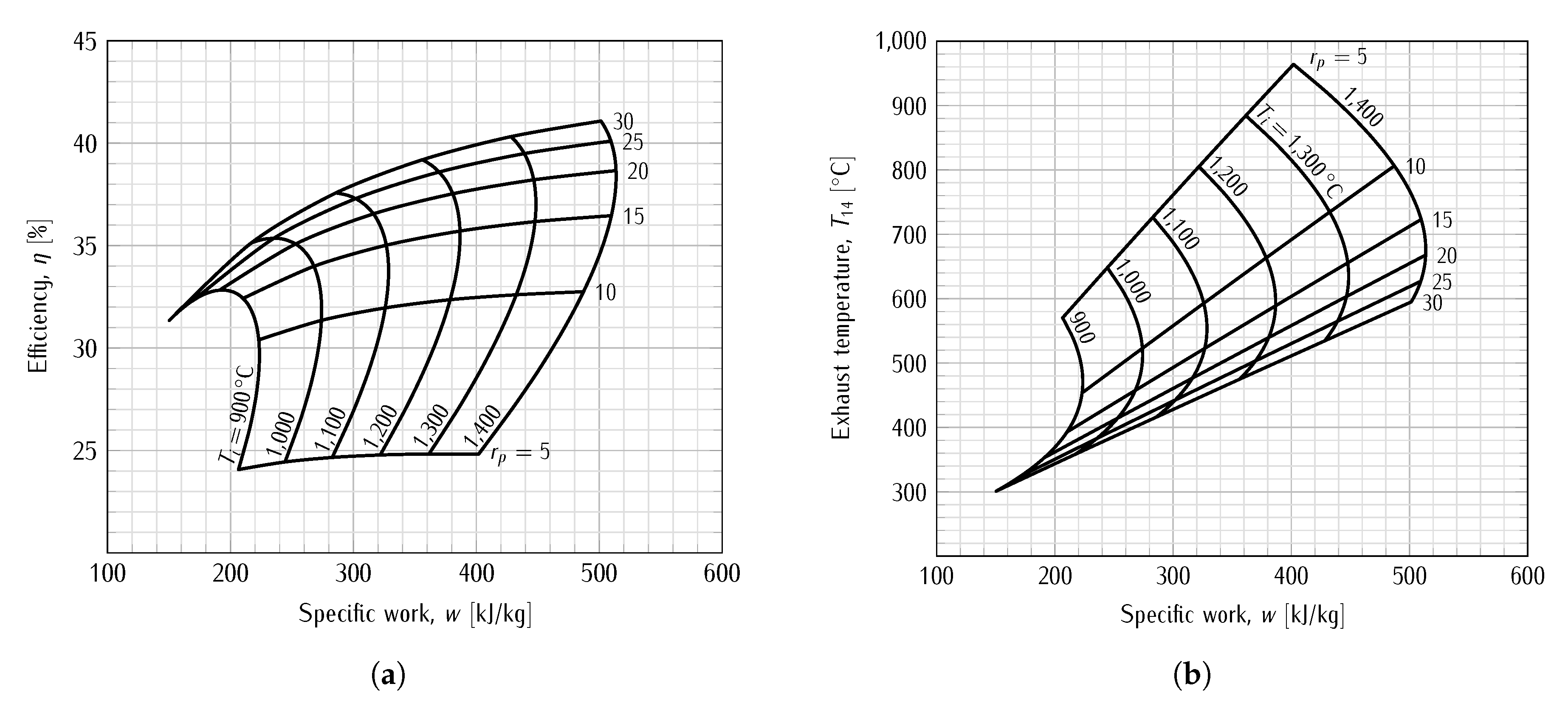
A standard gas turbine model consists of the following three components: air compressor, combustion chamber, and expander. It is defined by three design parameters: turbine inlet temperature (TIT), pressure ratio, and net power output. Even though the three-component standard design is often used for energy system analyses, its primary flaw is that the share of combustion in the total exergy destruction ratio is generally overstated because the exergy destruction caused by the mixing of cooling air, both in the combustion chamber itself and the expander, is not calculated separately. Sorgenfrei [37] presents an advanced GT model with three extractions from the compressor, providing cooling air for the combustion chamber and four turbine blade rows. With reference to this principle, a gas turbine model with a minimum of two cooling streams as seen in Figure 1 is presented in this paper. The $\lambda$-Mixer represents the cooling and excess air streams led into the combustion chamber with a given ratio. Rather than adding a physical component to the system, the mixer serves as a logical separator between two different processes taking place in the actual combustion chamber (CC), which is therefore represented as a whole by the gray-highlighted box. In the following, the term SC refers to the stoichiometric combustion process, modeled as a complete oxidation with the option of defining a relative heat loss that affects the outlet temperature of the combustion chamber (COT).

A similar principle applies to the second mixer added. The TIT-mixer subsumes the cooling air streams for the turbine blades according to the ISO 2314 standard. This norm describes a theoretical TIT as the result of an energy balance over the turbine inlets and outlets, including cooling air streams, see Reference [8] pp. 900–909. In this model, the TIT as a design basis parameter is given by the user while the corresponding mixing ratio and enthalpy are computed taking into account the chemical compositions of the cooling air and the exhaust gas. Absolute mass flows are then derived as a function of the second design-relevant parameter, the preset net GT power output. Exergy destructions caused by mixing hot exhaust gas with cooling air are evident in the difference between COT and TIT, which must be positive. The expansion process in the turbine is calculated with constant isentropic efficiencies. The same holds for the compressor which additionally uses the pressure ratio as the third design parameter set by the user.

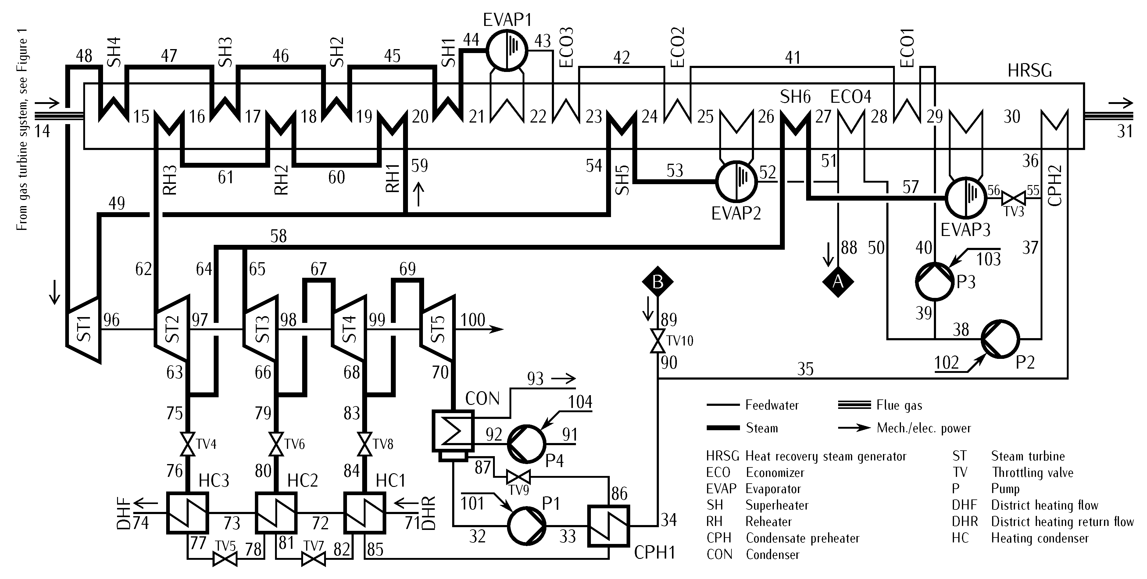
2.5. Heat Recovery Steam Generator and Steam Turbine

The gas turbine simulation can be expanded to a combined cycle process adding a water-steam-cycle heated by the exhaust gases. Required heat recovery steam generators can be assembled by arbitrary combination of the components evaporator and gas-water heat exchanger. They are modeled with energy balances over the cold and the hot fluid stream connected by the heat flow. Relative pressure losses must be set by the user.

Heat recovery steam generators with several pressure levels can be implemented. This can be achieved by arranging several steam turbine stages and assigning an inlet pressure to each. Pressure levels are then calculated upstream by means of the given pressure losses. Steam extractions are modeled with the division of one steam turbine into two stages with a splitter placed in between. The pressure of the steam extraction is given implicitly by the entering pressure of the following turbine stage.

Phase changes could occur in components like evaporators, condensers and low pressure steam turbines. Enthalpies and entropies for states in the wet steam region are calculated–if necessary–using the steam quality x as well as the enthalpy and entropy of saturated liquid and vapor.

2.6. District Heating

The component library includes heating condensers that enable the user to add a district heating system that uses extracted steam as a heat source. They can either be implemented individually or in a concatenated configuration, where the condensate of the heating condenser with the higher working pressure is throttled and led into the following one. The heating-circuit water mass flow is determined by the values of its target temperature and the total heat rate, both of which have to be preset by the user. As the individual target temperature behind each condenser depends on its user-defined percentage share of the total heat rate, the corresponding steam condensing pressure is variable. However, the extraction steam pressure is defined in the latter turbine stage, as it is assumed that simulations of plants with district heating systems should depart from a fixed steam turbine design in order to ensure comparability of different configurations or load cases. Consequently, a throttling valve (TV) has to be placed between turbine stage and heating condenser. For the phase changes in the heating condensers the statement given in Section 2.5 applies analogously.

3. Programming, Simulation and Calculation

This section outlines the procedure how a physical model is transformed into a running program to simulate a given process as described in general in Section 2 and in particular in Section 4. The source code examples that occur in this article are formulated according to the syntax of Python, see Reference [48]. It is an object-oriented programming language that allows global definitions to be used by various objects. Theoretically any other object-oriented programming language could be used. In this case it is necessary to verify whether it has the ability to import IAWPS and GERG libraries as well as a solver which operates similarly to fsolve. Within Python this nonlinear system solver is provided by SciPy, which is a Python-based system of open-source software for mathematics, science, and engineering, see Reference [49]. The solving algorithm is based on the software MINPACK. This is a numerical library which comprises various methods for solving systems of linear and nonlinear equations, see Reference [50].

The physical plant consists of components and the connections between them, the pipes. In a steady-state investigation the properties of the fluid in the pipes are constant. Each component and each state is reproduced as an object with different attributes and calculation methods. A structure matrix sets the connections between components. It serves as a basis of an equation system. This system consists of equations which are defined in the definition of the objects and, therefore, the classes. After iterative solving of the system of equations, all attributes of the components and states are determined and, therefore, the modeling is accomplished. In the following, the two major parts, the implementation of components and states as well as the solving algorithm are described in detail.

3.1. Implementation of Components and States

As introduced, the thermodynamic system is mainly characterized by its components, the links between them, the used working fluid(-s) and its operation mode. This subsection focuses on the implementation of components and states.

A class is an object which consists of attributes. Subclasses inherit the attributes from their primary class and also have new attributes. Therefore, the same definitions of attributes and equations are not required to be rewritten for every single object. Subclasses are created for every component and fluid (state) of the system. Here, two primary classes are fundamental: state and component. Initial and boundary conditions are set within subclasses. More specifically, the thermodynamic system consists of a large number of components. However, the number of component types is limited to only a few. Most of the attributes and calculation methods for different components equal each other. Therefore it seems to be beneficial to undertake definitions of attributes and calculation methods only once. General definitions are positioned in the superior class component. More detailed definitions may be defined in classes of the exact component types. At the lowest level, there could also be component-specific definitions.

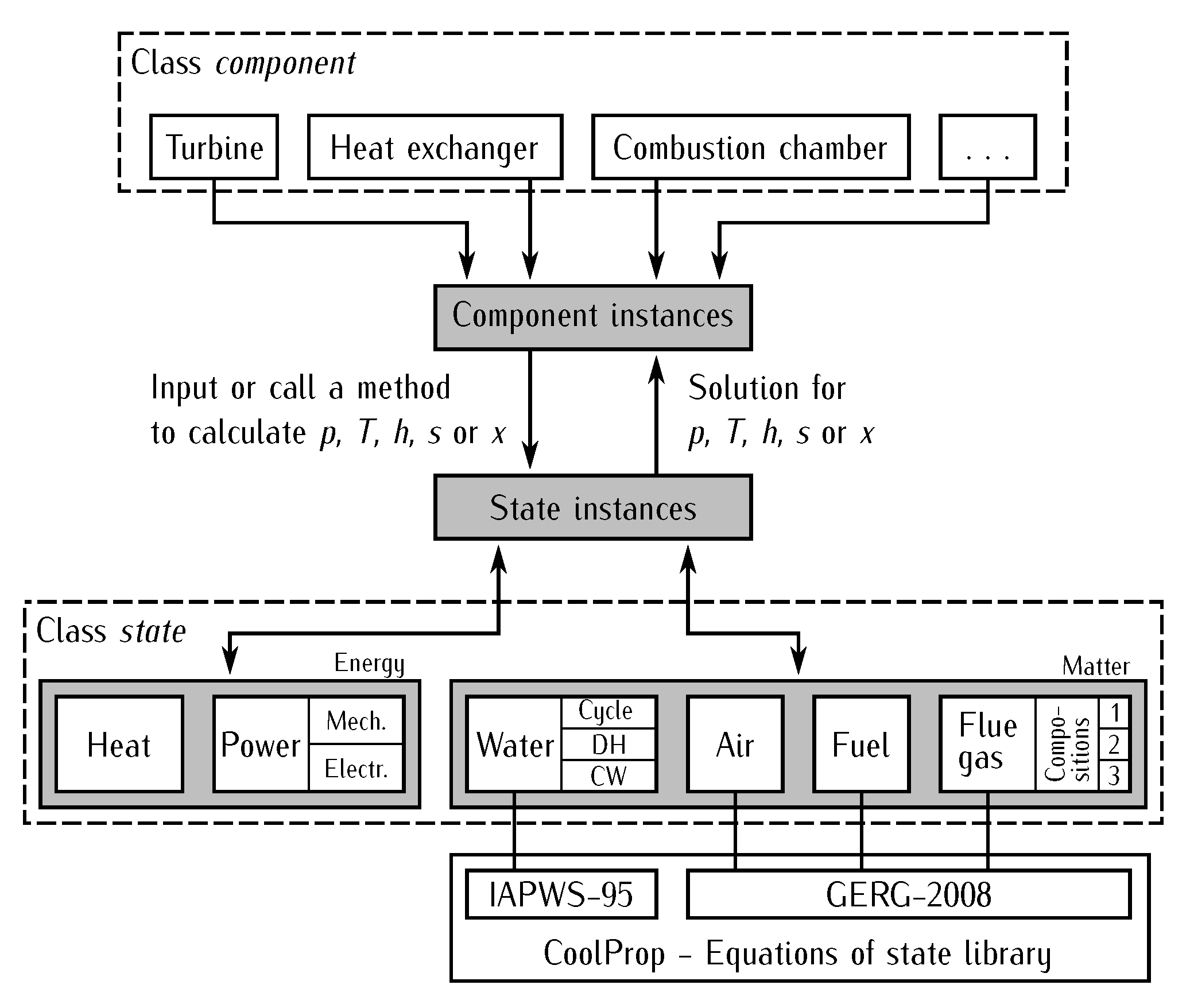
Figure 2 shows the principle of interaction between instances of state and component classes in a simplified way. In the following, the classes are described in particular. The connection between components can be work rates, heat rates or material streams. As described above, in a steady-state investigation the properties for material streams are called states and stay constant over time. Variables which characterize fluids are pressure, temperature, enthalpy, entropy, and chemical composition. Within subclasses of components an access on these subclasses of states takes place. There are various types of subclasses defined such as water, air, fuel, flue gas, heat and mechanical as well as electrical power. The fuel subclass allows the calculation of a stoichiometric demand of oxidizer required, based on the chemical composition of the fuel. The air subclass calculates the composition of air with respect to air humidity. Due to the fact that there are two feed-ins of cooling air, the flue gas exists in three different compositions. Hence, also three subclasses for flue gas are defined. In a similar way there are three different subclasses for water defined; cycle water, water for district heating, and cooling water. They are all considered to be pure fluids. Possible missing properties are calculated with equations of state as mentioned in Section 2.3 and then overwritten in the specific subclass. Apart from their chemical composition, two properties of state are required to calculate the remaining properties.

Equations required for the physical modeling of components are implemented in the related subclasses. These subclasses inherit the attributes and methods of the superior class component. These are names of components, lists of inlet and outlet streams, and various exergetic values and ratios. For instance, isentropic efficiencies will be added in the specific subclass. The defined equations in the subclasses are accessed by the system of equations. Component specific equations determine the impact a component has on its inlet or outlet streams. These methods are sorted into different categories which are discussed later.

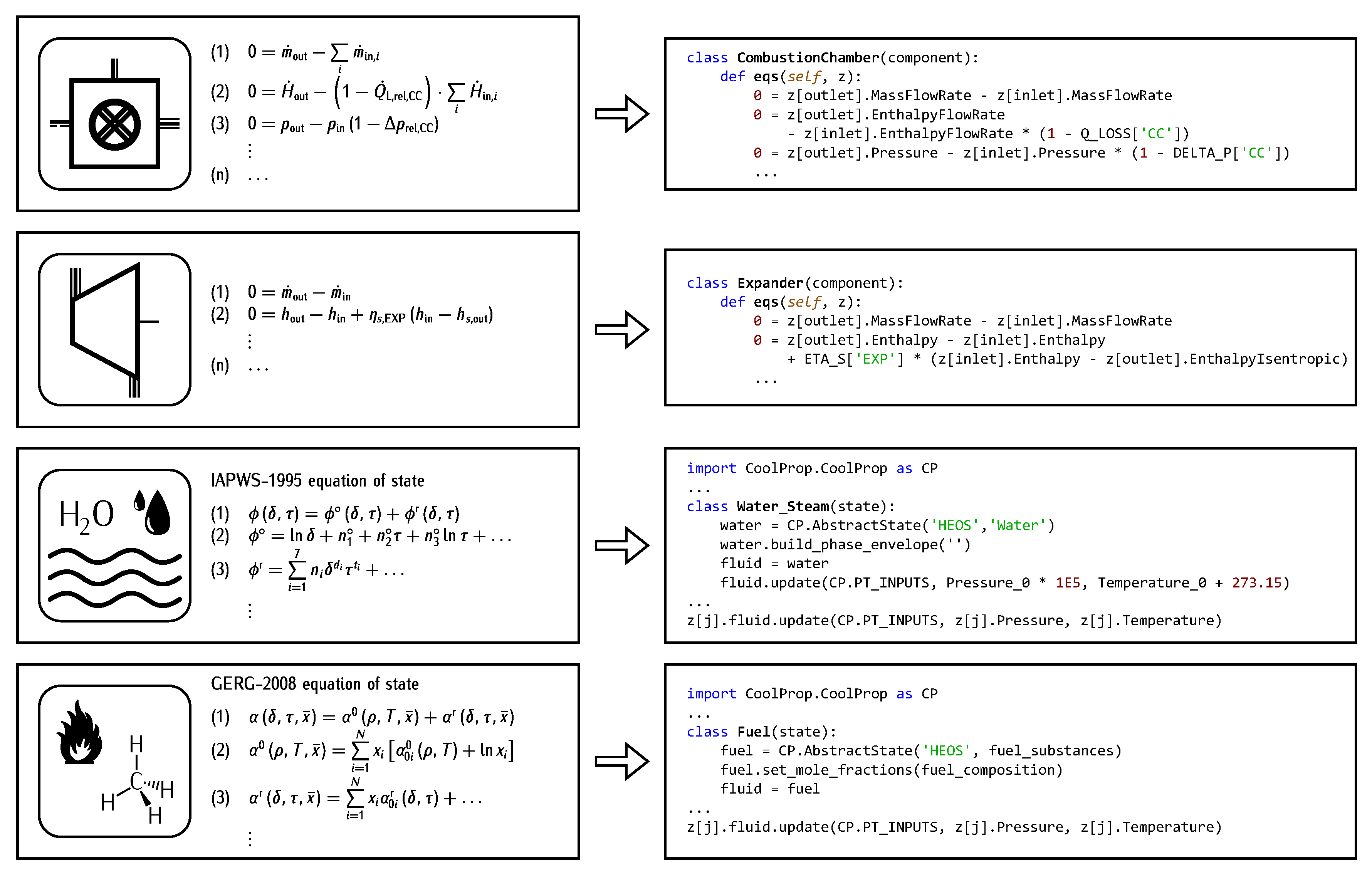
Figure 3 shows a few simplified examples on how the physical model for components and states is translated into Python code. The variable z represents all states. With square brackets containing inlet or outlet stream numbers and dot with called attribute or method afterwards, a property of a specific state is retrieved.

3.2. Solving Algorithm

In general, a simulation is the creation of an equation system and its solution. It represents a simplified reflection of a real power plant. More precise, the focus here lies on the steady-state thermodynamic process. Hence, the equations are based on the modeling of the process. In fact, at first components must be modeled and structured in order to determine the plant’s behavior. To assign equations to components and states, it is crucial that they are numbered, see Reference [51] pp. 588–604.

Basically, steady-state processes can be solved in two ways. Intuitively, a sequential modular approach seems straightforward. Unfortunately, a disadvantage is that the output is a function of the input and that inputs often depend on components that follow the current considered component. Thus, explicit iterations loops are required which can be excessively complex for processes with a large number of connected components and recirculating streams, cp.Reference [52] pp. 88–91.

In contrast to the method described above, a simultaneous modular approach is more advantageous in terms of implementation for this setting of a power plant process. The system of equations is solved simultaneously under the condition that dependencies between inputs and outputs for components are defined. In that way an input is also a function of the output. However, simultaneous iterative calculations with nonlinear equations for processes with a large number of components result in an excessive computing effort. This is also true for the applied solving algorithm fsolve, which is not able to compute all equations at once. As a consequence, the system of equations is split into different modules which are solved sequentially. Within one module the solution is determined simultaneously. The fragmentations consist of component groups and energy and mass balances. A disadvantage for this approach is the difficulty of localizing possible upcoming convergence errors, see Reference [52] pp. 92–94. Simultaneous solutions of nonlinear equation systems are based on Newton’s method. In principle it is about finding the root of a continuous function carried out using the tangent method.

As introduced, the simulation is split into four parts. First, inlet pressures and losses are given within certain states and components, respectively. In that way, all other pressure levels can be determined and, if possible, temperatures of evaporation processes, too. Second, enthalpies and entropies are determined by calculated pressures and given temperatures, with the exception of enthalpies and entropies which depend on mass flow ratios such as mixing of streams or heat transfer. Third, almost every mass flow rate for the process is determined. The focus is on the calculation for the air and flue gas mass flow in the gas turbine. Fourth, remaining mass flow rates are determined for steam turbines and district heating condensers. The heat transfer areas for heat exchangers and steam qualities are also calculated. After the execution of these four steps an exergy analysis takes place. It is not part of the equation system. This is due to the fact that exergy is not part of the modeling of the process but rather serves for its evaluation. For each part an encompassing array is created with particular equations for each component as entries. The nonlinear system solver is used with reasonable start values.

A structure matrix indicates in which order and by what matter components are connected. Based on this process, characteristic instances of classes are created for components and states. This is a replacement for a graphical flowsheet. For state variables which are unknown, a certain negative value A is assigned. This serves as a placeholder for further calculations. At some point of the calculation the value A of the state variable is required to calculate another value B. Before this happens, it is required to check whether value A has been changed to a positive value by another method. If yes, value A can be used by a method to calculate value B. If not, both values can only be determined by a method later in the calculation. The given parameters for the components are saved in the particular component. Parameters in conjunction with states are saved directly in vector z. With queries it can be ensured that solely parameters and guessed values are used to calculate the solution of the equation system.

As mentioned in Section 1, CoolProp is used to calculate state variables of a fluid as a function of two other state variables. Numerical calculation methods of gas mixtures are more complex in comparison to pure fluids. Therefore the only state variables which can be given as input are temperature, pressure, and steam quality. Since energy balances are widely used to describe the thermodynamic process, many equations contain enthalpies and entropies. To use these state variables as input for CoolProp, an aid method is implemented. In principle, this method iteratively determines a temperature as a function of pressure and enthalpy or entropy. Therefore, again fsolve is used. Thereby, the limitation of CoolProp is bypassed.

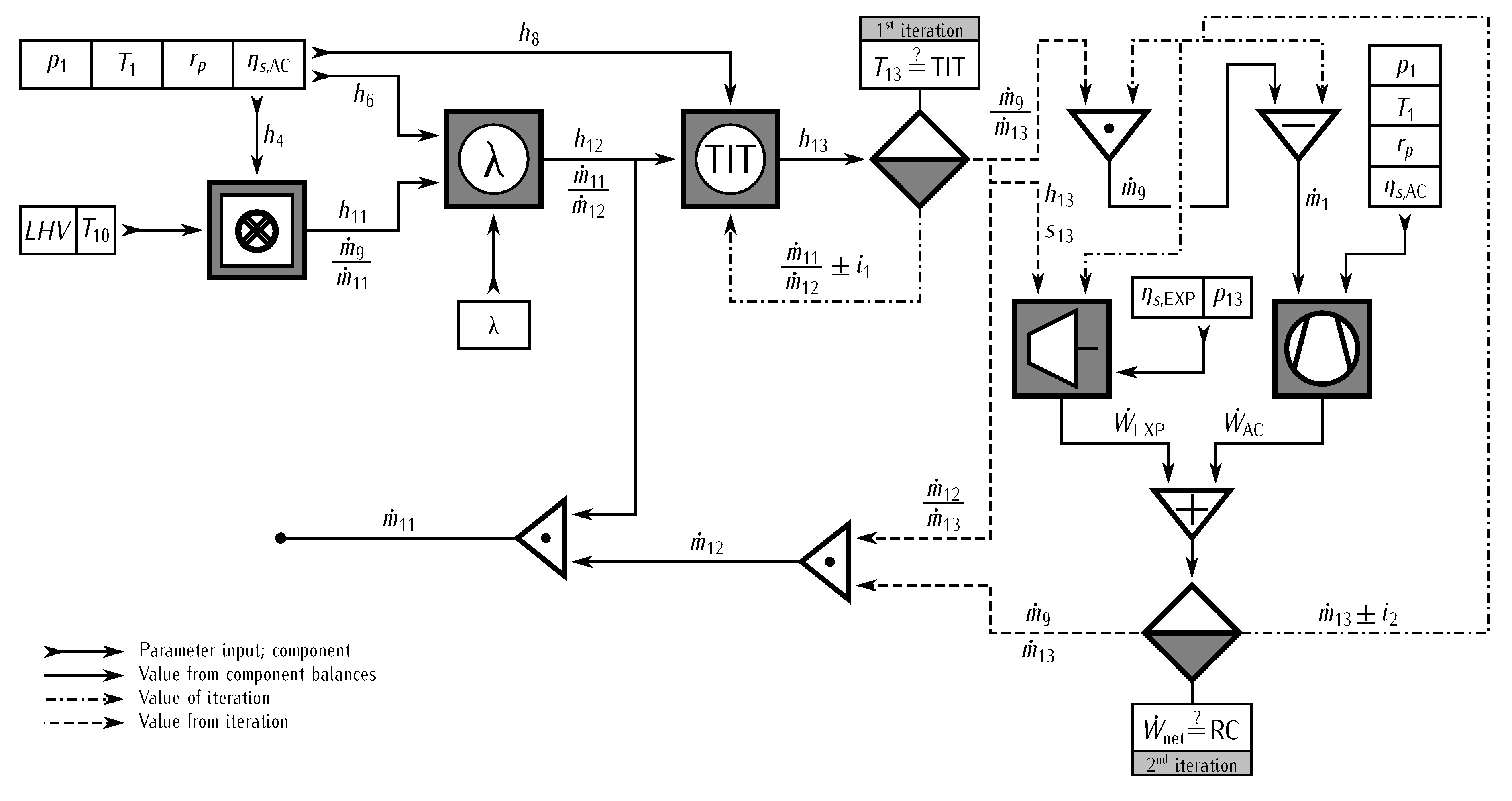
Similarly to the example above, certain methods are required in order to model the system. This example showcases the correlation between different variables and parameters. These correlations are not always trivial. Therefore the calculation time is decreased by implementing a specific control scheme which includes the indirect method as described above. The turbine inlet temperature is one of the major characteristics of the gas turbine as described in Section 2.4. The real TIT is not explicitly measurable. According to ISO 2314 standard, it is rather defined as a temperature which represents a theoretical TIT. It would arise as a mixture of flue gas at the outlet of the combustion chamber and entire cooling air at once. In this case, TIT and the net power output are parameters given externally. The required mixture ratio of mass flow rates 8 and 11 is determined according to Figure 4. It represents the iterative method of the calculation of variables based on given parameters. The two connected iterations end if the computed TIT equals the given input and the sum of the power of expander and compressor equals the given net power.

4. System Analysis of Model Case

The simulation presented in this paper is based on models of the main components that constitute a simple or combined cycle gas turbine power plant (CCGT). Therefore, CCGTs can be assembled and simulated in different configurations. The analysis in this paper is mainly conducted on the basis of a model case CCGT with a three-pressure HRSG and a district heating system, as illustrated in Figure 1 and Figure 5. The gas turbine system includes two bypass flows which represent the combustion chamber and turbine blade cooling streams as well as a fuel preheater (FPH) working with extracted intermediate-pressure steam. For assessments of a simple cycle GT, the FPH has to be omitted. To ensure an efficient adaption to the flue gas temperature curve with low temperature differences, the economizer and superheater sections of the high-pressure and the reheat stage are divided into several heat exchanger segments. Besides the evaporator (EVAP1), the high-pressure stage consists of three economizers (ECO1 to ECO3) and four superheaters (SH1 to SH4), while the intermediate-pressure stage includes one economizer (ECO4), an evaporator (EVAP2) and a superheater (SH4), respectively. Intermediate-pressure steam is mixed with cold reheat steam and passes three reheaters (RH1 to RH3). Additionally, there is a low-pressure stage consisting of an evaporator (EVAP3) and a superheater (SH6). The superheated steam is mixed with the main steam flow before entering the low-pressure steam turbine (ST3 to ST5). The turbine train is completed by the high-pressure (ST1) and the intermediate-pressure turbine (ST2). The district heating system raises the heating-circuit water to the target temperature using three heating condensers (HC1 to HC3) which are fed by steam turbine extractions on successive pressure levels.

Parameters used for the system analysis are listed in

Table 1. Assumptions and given parameters.

Ambient conditions
Air state	$T_0=5{}^{\circ }$C, $p_0=1.013\mathrm{bar}$, $\phi =75\%$
Composition of dry air	78.09% N2, 20.95% O2, 0.03% CO2, 0.93% Ar
Cooling water	$T_{91}=8{}^{\circ }\mathrm{C}$, $\Delta T_{\mathrm{CON},\max }=6\mathrm{K}$
Gas turbine system
Design parameters	${\dot{W}}_{\mathrm{net}}=400\mathrm{MW}$, $TI{T}_{\mathrm{iso}}=1340{}^{\circ }\mathrm{C}$, $r_p=19$
Efficiencies	${\eta }_{s,\mathrm{EXP}}=0.89$, ${\eta }_{s,\mathrm{AC}}=0.875$, ${\eta }_{\mathrm{mech}}=0.995$, ${\eta }_{\mathrm{vol}}=0.995$
Combustion	$\lambda =1.9$, $\Delta p_{\mathrm{rel}}=5\%$, ${\dot{Q}}_{\mathrm{L},\mathrm{rel}}=2\%$
Lower heating value of fuel	$LHV=39.89\mathrm{MJ}/\mathrm{kg}$
Composition of fuel	83.38% CH4, 10.3% N2, 3.6% C2H6, 1.8% CO2,
	0.6% C3H8, 0.2% C4H10, 0.07% C6H14, 0.05% C5H12
Fuel preheating	$\Delta T_{\mathrm{FPH}}=190\mathrm{K}$
Bottoming cycle
Water live (reheated) steam	$p=170\mathrm{bar}\left(34\mathrm{bar}\right)$, $T=600{}^{\circ }\mathrm{C}\left(600{}^{\circ }\mathrm{C}\right)$
Turbine inlet pressures	$p_{\mathrm{ST}3}=4.5\mathrm{bar}$, $p_{\mathrm{ST}4}=2\mathrm{bar}$, $p_{\mathrm{ST}5}=1\mathrm{bar}$
Efficiencies	${\eta }_{s,\mathrm{ST}}={\eta }_{s,\mathrm{P}}=0.9$, ${\eta }_{\mathrm{mech}}=0.995$, ${\eta }_{\mathrm{vol}}=0.995$
Heat exchangers (general)	$\Delta p_{\mathrm{water},\mathrm{rel}}=1.0\%$, $\Delta p_{\mathrm{fg},\mathrm{rel}}=0.2\%$, $\Delta T_{\min }=10\mathrm{K}$
Evaporators	$\Delta p_{\mathrm{water},\mathrm{rel}}=3.0\%$, $\Delta p_{\mathrm{fg},\mathrm{rel}}=0.3\%$, $\Delta T_{\min }=15\mathrm{K}$

. Net power output, TIT, and pressure ratio, as the three main design parameters of the GT, are particularly important because they define the plant dimension. It is assumed that all components except SC are adiabatic. The condenser is assumed to be a dissipative component.

5. Results from Model Case

Besides the validation of the GT model, this section contains an exergy analysis of the model case process presented above with a focus on the GT components. A sensitivity analysis concerning the impact of heating load distribution between the HCs on exergetic efficiency follows.

5.1. Validation

The GT model without fuel preheater is validated by plotting the simulated net efficiency and the exhaust gas temperature against the specific work for different turbine inlet temperatures and pressure ratios. Figure 6 shows the resulting characteristic maps which manifest high qualitative and quantitative conformity with literature data, cp. Reference [8] p. 30. The curves for a constant TIT with varying pressures show a parabolic path with diminishing positive correlation between pressure ratio and efficiency growth. Lower TIT curves clearly show a decrease in efficiency after having reached its maximum value, which for increasing temperatures lies at much higher pressure ratios than those simulated. For a simulated TIT of 1400 ${}^{\circ }$C, which is a value consistent with state-of-the-art GT technology, the resulting simple-cycle energetic efficiency for usual pressure ratios lies in the range of 38–41%. For higher temperature levels with significant blade cooling, the theoretical TIT calculated with ISO 2314 is 150–200 ${}^{\circ }$C lower than the COT, see Reference [53].

5.2. Exergy Analysis

A common result of the exergy analysis within scientific literature is that the main exergy destruction occurs during combustion in energy conversion processes. Due to the smaller role of heat transfer compared to steam power plants, this is especially valid for gas turbine processes. Ganjehkaviri and Jaafar [54], Khaldi and Adouane [55] as well as Song et al. [56] execute exergy analyses of open-cycle GTs operating at full-load in the net output range of 107–150 MW and come to the conclusion that the CC is accountable for 78–85% of the total exergy destruction in the system, values that coincide with the simulation result of 78.6% for the open-cycle GT simulation with a rated capacity of 400 MW. These values, however, do not offer conclusions about the shares of the different processes contributing to the exergy destruction in this component; Seen individually, they can lead to the misinterpretation that the combustion reaction alone is responsible for this amount of exergy destruction. Tsatsaronis et al. [57] present an exergy-based concept of dividing the inefficiencies in combustion processes into their respective causes, namely friction, mixing at different temperatures, and chemical reaction. Additionally, an exergy loss of 2% (heat transfer to the environment) was considered in the present case. The split of the CC into different components described in the system analysis follows the logical differentiation of the causes for exergy destruction. Consequently, the Grassmann diagram, which is derived from our exergy analysis and presented in Figure 7, shows that even if the stochiometric combustion reaction is in fact the most important inefficiency with a share of 79% of total exergy destruction in the combustion process, the mixing of excess and cooling air and the pressure drop caused by friction also contribute with respective shares of 18% and 3%.

The differentiation between two different sources of exergy destruction in the turbine, polytropic expansion and mixing at different temperatures, follows the same pattern with the latter source being caused by the addition of blade cooling air. In this way, Song et al. [56] examine the exergy destruction caused by the cooling of the turbine’s blade rows. In the present paper, the blade cooling air streams are aggregated to one and integrated with the TIT-mixer following the aforementioned ISO 2314 standard. The results show that almost one third of the exergy destruction in the turbine is caused by mixing the hot combustion gas with the induced cooling air.

Compared to an open cycle configuration, the exergy analysis of the GT system only changes slightly for the CCGT process depicted in Figure 5. First, due to pressure losses in the HRSG, the expansion does not end at ambient pressure. Therefore, a higher air mass flow is required for a constant net power output of the GT. Second, fuel preheating with intermediate-pressure water is implemented, which on account of a lower temperature difference between air and fuel lowers the exergy destruction during combustion by almost 3% (approx. 10 MW). While 36% of the total fuel exergy are converted to shaft work in the GT system, 33% are destroyed and 2% lost to the environment, only 29% remain in the exhaust gas. As stated by Kail [58] in his assessment of three-pressure CCGTs, the exergy flow in a process decreases much faster than the energy flow, because exergy destruction occurs in each component, whereas energy loss is only identifiable in flows to the environment. Almost three quarters of the exergy remaining in the exhaust gas are converted to shaft work in the steam turbine via HRSG and water-steam-cycle or to heat output in the district heating system, while about 5% are lost in the exhaust gas led to the stack. From this follows that the exergy destruction in the entire bottoming cycle only amounts to less than one fifth of the GT value. As visible in the Grassmann diagram, 30% of this exergy destruction originates from steam turbines including the condenser and 15% from district heating, while 55% are caused by heat transfer within the HRSG. Here, the contribution of CPH2, which lies in the same $y_D$-range as the high-pressure and the intermediate-pressure heat exchangers, is noteworthy. The disproportionate exergy destruction in this heat exchanger is caused by the low operating temperatures on both sides.

5.3. Sensitivity Analysis of the District Heating System

The three-stage district heating station included in the CCGT deserves a closer look. To achieve the most efficient use of the three extractions from the steam turbine, the optimal distribution of the heating load between the HCs has to be found. As stated in Section 2.6, the simulation of the HCs departs from the extraction pressures defined in the steam turbine section. For the district heating analysis, these pressure levels partly diverge from the parameters given in Section 4: They are set to 5, 2 and 1 bar, respectively. Furthermore, the supply temperature is lowered to 115 ${}^{\circ }$C.

Considering this target supply temperature, the minimal temperature difference of 3 K in the condensers, and the condensing temperature at the HC1 working pressure of 1 bar, it is apparent that this HC cannot sustain the heating load by itself. Its contribution to the heating supply is supposed to be limited to 60%, whereas the other HCs can each supply up to 100% of the heating load. The sensitivity analysis considers the total exergy destruction in the HCs and the exergetic efficiency of the CCGT plant, respectively. The possible heating supply distributions between the three HCs span a triangular array. A total of 56 load distributions within this array served as a basis for the sensitivity analysis. Departing from the simulations for these points, the results for every possible load distribution were interpolated. The results of the analysis are shown in Figure 8.

Figure 8a shows a circular display of increasing exergy destruction rates departing from the minimum point at a relatively even distribution of the heating load (40%, 30%, 30%) with a concentration of the supply to only one HC showing the highest exergy destruction rate. This result is caused by the correlation between exergy destruction and mean temperature difference of heat transfer, which reaches lower values for even distributions. In contrast, the concentration of the load to one HC increases its mean temperature difference. Nevertheless, the optimal distribution is not the perfect even one. The light offset of the circular display towards higher shares of HC1 shows that the corresponding increase in temperature difference within this HC is to some extent outweighed by the successive decrease in the following HCs. Still, the sensitivity analysis based on the combined exergy destruction of the HCs points to the conclusion that even distributions should be preferred.

However, if one takes a broader look at the system, this conclusion must be refuted. It is apparent in Figure 8b that the optimal working point for the entire system is reached where the capacity of the HCs with the lowest working pressures is exploited first. The lines of constant efficiency form a diagonal front descending from the optimum at a load distribution of 60%, 40%, 0% to lower values with a slope that is slightly tilted towards HC1. The reason for this trend is that extraction and required condensing pressure are significantly closer to each other for the HCs working on lower pressure levels. Consequently, exergy destruction caused by throttling extracted steam in the upstream TVs is much lower. This effect outweighs the increase in temperature difference by concentrating on one HC, which is observed on the specific component level. The district heating example shows that the comprehensive look on the entire system offered by the exergy analysis uncovers optima which would not be detected in a purely component-wise study.

6. Conclusions

The present paper motivates the use of an open-source framework for the simulation and exergy analysis of energy conversion processes. A literature review collects the recent developments in the field of gas turbines, exergy-based methods and open-source frameworks for the thermodynamic simulation of energy conversion processes. The basics of thermodynamic modeling and exergy analysis as well as the assumptions for fluid properties are mentioned. As an example of an energy conversion processes a combined cycle gas turbine is presented. The model of the system is described along its main component groups. Aspects of programming, simulation, and calculation are shown in principle and transferred to the model case. For the sophisticated gas turbine model, the iterative determination of the mass flow rates is shown in a calculation scheme. Based on the given assumptions, flow sheets, and parameters the validation and results are presented.

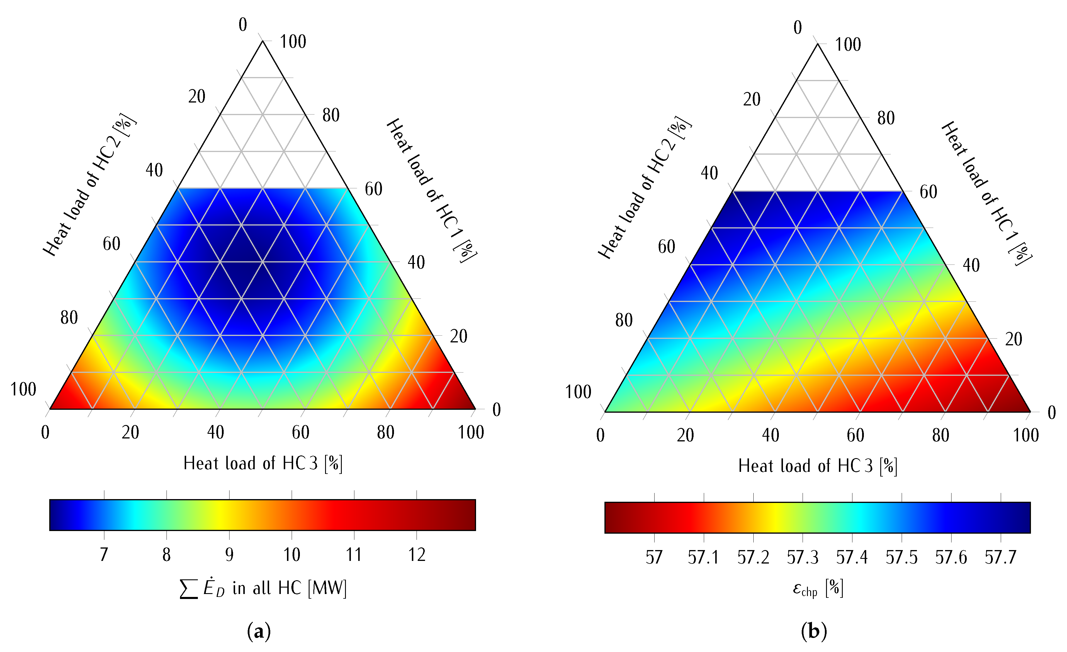
The study shows that simulations and exergy-based analyses of energy conversion systems are possible in an open-source framework. As an example this paper shows the solution of a state-of-the-art combined cycle using a more precise gas turbine model and sophisticated equations of state. The gas turbine model is validated with literature data. The results of the exergy analysis—shown in a Grassmann chart—represent the level of detail of the model. In particular, the causes of the exergy destruction rate in the combustion chamber can be quantified accurately and corresponds to the data published previously in literature. An exergy-based sensitivity analysis of the district heating system shows that minimizing the exergy destruction rate in the heating condensers does not necessarily lead to a better overall exergetic efficiency. The interactions between steam extractions and net power output have to be considered in a CHP plant. Finally, the analysis shows a high degree of agreement with already known results. The necessary extractions along the turbine shaft to fulfill the heat demand, should be done as late as possible.

In future research the open-source framework—shown in this paper—could be used for other energy conversion systems as well as part-load analysis. Furthermore, the approach will be extended to exergoeconomic and advanced exergy-based analysis. Since the thermodynamic model is available in an object-oriented formulation, not only a rapid expansion or changes of the components are possible, but also the transition from simulation to optimization is facilitated.