Decentralized Energy Management of Networked Microgrid Based on Alternating-Direction Multiplier Method

Abstract

With the ever-intensive utilization of distributed generators (DGs) and smart devices, distribution networks are evolving from a hierarchal structure to a distributed structure, which imposes significant challenges to network operators in system dispatch. A distributed energy-management method for a networked microgrid (NM) is proposed to coordinate a large number of DGs for maintaining secure and economic operations in the electricity-market environment. A second-order conic programming model is used to formulate the energy-management problem of an NM. Network decomposition was first carried out, and then a distributed solution for the established optimization model through invoking alternating-direction method of multipliers (ADMM). A modified IEEE 33-bus power system was finally utilized to demonstrate the performance of distributed energy management in an NM.

1. Introduction

1.1. Motivation

With ever-increasing installations of distributed generators (DGs) and the implementation of advanced metering/monitoring infrastructures, a distribution power system in general is undergoing a transition from a hierarchical structure to a distributed one [1]. Consequently, a networked microgrid (NM), an interconnection of multiple microgrids, has emerged as a new distributed paradigm. It has been shown that an NM can offer more reliable and economical energy supply with lower operational costs [2]. In addition, the NM could maximize the asset utilization of DGs and thereby reduce greenhouse gas emissions.

However, for a geographically dispersed NM including a variety of dispatchable DGs (e.g., wind turbines and diesel generators), the centralized approach requires significant investment for implementing the control center as well as communication infrastructures [3,4]. Furthermore, storing all data in one control center carries the risk of exposing the privacy of customers, as well as unavoidable single-point failures [3]. More importantly, the distributed method is more computationally efficient than the centralized one. Therefore, it is desirable to effectively coordinate NMs in a distributed manner for improving reliability and economics.

1.2. Literature Review

Conventionally, a distribution-level microgrid is centrally controlled by a central coordination center [5]. More specifically, the central coordination center collects relevant information from dispersed controllable devices and forecasting data to perform an optimal dispatch of distributed resources for the next period [6]. Centralized energy-management architecture has been widely studied in existing publications. Reference [7] proposed a two-layer energy-management model wherein the schedule level attains the economic-operation scheme based on forecasts, while the dispatch level dispatches controllable DGs based on real-time data. In Reference [8], a centralized scheduling algorithm was proposed for an electric vehicle-dominated microgrid to optimize the charging scheme considering the charging cost and convenience of microgrid users. In Reference [9], the centralized energy-management problem for a household-level microgrid was formulated as a utility-maximization problem, subject to capacity constraints. In Reference [10], a centralized energy-management optimization model was formulated for a residential-quarter microgrid including a concentrating solar-power unit with an objective of minimizing the involved operation costs. A two-stage stochastic demand-side management model for a commercial-building microgrid is formulated in Reference [11], considering the uncertainties in solar-generation outputs, loads, microgrid availabilities, and microgrid energy demands.

The fully distributed optimization method includes two broad categories, i.e., the Lagrangian relaxation-based and the optimality-condition decomposition-based category. The Lagrangian relaxation approach formulates the Lagrangian function and then solves the subsequent dual Lagrangian relaxation problem by two steps in an iterative process: (1) decomposition of the relaxed primal problem with given multipliers; and (2) update of multipliers. Note that the multiplier-update technique commonly includes the subgradient method, cutting-plane method, bundle methodm, and trust-region method. Readers can refer to Reference [12] (Chapter 5) for details. To enhance the convexity of the relaxed primal problem and improve the convergence, a quadratic penalty term is conventionally added in formulating an augmented Lagrangian function. The auxiliary problem principle is then employed to linearize the augmented Lagrangian function so as to decompose the relaxed primal problem into several subproblems, which is thus called as augmented Lagrangian decomposition [13,14]. In addition, similar to augmented Lagrangian decomposition, the analytical target-cascading method generally decomposed a system into a multilevel hierarchical structure through introducing penalty functions to model autonomous interdependencies [15]. The penalty function is usually modeled as an augmented Lagrangian block coordinate-descent formulation or exponential penalty function, which consequently brings many parameters to be tuned. The optimality condition decomposition-based approach is initially proposed for solving large-scale nonlinear and possible nonconvex problems in Reference [16]. Specifically, it solves the first-order Karush–Kuhn–Tucker conditions in a distributed manner. Similar to optimality-condition decomposition, a heterogeneous decomposition is presented in Reference [17] to solve the optimal power flow for transmission and distribution systems. Reference [18] improves the convergence of optimality-condition decomposition by adding a correction term in the update process. However, the convergence conditions of optimality-condition decomposition are still not easy to verify for practical applications.

As a version of the augmented Lagrangian decomposition algorithm, the alternating-direction multiplier method (ADMM) overcomes the poor convergence problem of conventional Lagrangian relaxation approaches with only one parameter (i.e., the step size of the penalty term) to be tuned, which is thus widely applied in power-system optimization problems and machine learning in computer science. Many publications are available on ADMM-based optimization methods. For example, an ADMM-based distributed optimization is proposed in Reference [19] to facilitate transactive energy trading in distribution networks. The work in Reference [20] provides a distributed energy-management scheme for multiple interconnected microgrids in a real-time market. In References [3,21], an ADMM-based decentralized method of voltage control is proposed by only using the self-information exchange with neighboring regions. In Reference [4], a distributed method is proposed to carry out tie-line scheduling, taking into account uncertainties, for example, wind-output power. The work in References [22,23] formulates the optimal power-flow problem as a semidefinite programming one.

As power-flow equations are quadratic of bus voltages, power-system-operation optimization problems are mostly nonconvex. The conic-relaxation technique is commonly used to relax and convexify the nonconvex equations into a second-order cone (SOC) form [24,25,26]. The work in Reference [23] verifies that there exists a very small gap between the conic relaxation-based results and nonconvex power-flow-based ones for most actual distribution networks. In Reference [3], the conic-relaxation technique is applied to transform a voltage-control model into an SOC-programming model. Reactive power control is cast as an optimal power-flow problem in Reference [25], and the obtained nonconvex problem is equivalently transformed into an SOC problem. The work in References [25,26] provides less restrictive but sufficient conditions to guarantee exact SOC relaxation.

Additionally, power-industry deregulation provides opportunities for microgrids to schedule power consumption and reduce operation costs by direct participation in electricity markets [27,28]. Note that market transactions are still handled by a central coordination center [5]. Two market mechanisms are proposed in Reference [29] to solve the energy-management problem of the low-voltage distribution-level microgrids. More specifically, the microgrid operator constructs a local market, whereby DGs and consumers could bid their production and consumption in the first market mode while the microgrid could sell/buy active/reactive power to the upstream distribution grid in the second market mode. In Reference [20], it is assumed that the microgrid operator can sell or purchase energy from neighboring microgrids and the upstream energy market to minimize operation costs of NMs. In Reference [30], the microgrid takes part in a pool market and actively responds to the electricity price so as to maximize its total profits through coordinating controllable resources. Similarly, it is assumed that the NM operator in this work could participate in the real-time electricity market and thereby it is demanded to determine the energy-procurement scheme according to the forecasts of the real-time electricity price.

1.3. Contributions

Given the above background, a distributed energy-management model is presented with an objective to minimize the total operation costs of NMs. More specifically, the interconnected microgrids are decoupled and, subsequently, an ADMM-based distributed algorithm is employed to solve a decentralized energy-management model that just requires exchanging limited information among neighboring microgrids. The presented model is capable of protecting the privacy of customers and robust against communication failures (e.g., packet drops).

The main contributions of this paper include two aspects:

(1)

The established optimization model is reformulated into a convex one by employing a second-order cone-relaxation technique. Additionally, an ADMM-based solution method is utilized to solve the presented optimization model in a fully distributed manner with limited information exchange among neighboring microgrids.

(2)

The method in this paper can effectively accommodate an arbitrary number of controllable devices given an ever-increasing penetration of distributed energy resources in a microgrid, and thus greatly explore the potential benefits of DG applications.

The remainder of this paper is organized as follows: An SOC programming formulation of the energy-management problem is presented in Section 2 through relaxing power-flow equations. An ADMM-based distributed solving method is presented in Section 3. Case studies are conducted in Section 4 to validate the established optimization model and the presented solving method. In Section 5, conclusions are drawn, and future research work is prospected.

2. Mathematical Formulation

Power-industry restructuring introduces different electricity-market structures. In some electricity markets, both day-ahead and balancing markets are included [20], while in other electricity markets, such as the National Electricity Market of Singapore, bids for energy and ancillary services are cleared in a real-time fashion. Here, it is assumed that each NM participates in an electricity market similar to a microgrid.

Note that all participants in a microgrid are allowed to change their bids up to 65 min before the market closure. The market is cleared hourly, and energy-price forecasts for the following 24 h are provided based on standing bids. Thus, it is assumed that energy prices in our model are taken from the forecasts and the energy-management problem of an NM can be solved in a rolling manner. Specifically, the operator of NMs runs optimization routines hourly and bids its power consumption in the real-time market. In practice, a rolling approach can effectively mitigate the impact of uncertainties by using the updated forecasts, and thereby reduce the operation cost of the NM.

2.1. Objective Function

Here, two types of DGs are considered, i.e., fuel-based DGs, such as diesel generators, and renewable-energy-resource (RES)-based DGs, such as wind turbines and photovoltaic arrays. Note that it is assumed that fuel-based DGs are owned by microgrids for simplicity. The objective in the proposed optimization model is to minimize the total operation costs, which comprises three parts: the fuel cost $f(P_{g,t}^{G,a})$ of fuel-based DGs, the cost of purchasing the energy from the main grid ${\lambda }_t^{}{P}_{a,t}^M$, and the cost of purchasing energy from RES-based DGs, formulated as:

$$\min {\displaystyle {\sum }_{a\in \mathbf{N}}{\displaystyle {\sum }_{t\in \mathbf{T}}\left[{\displaystyle {\sum }_{d\in {\mathbf{N}}_a^G}f(P_{d,t}^{G,a})}+{\lambda }_t^{}{P}_{a,t}^M+{\displaystyle {\sum }_{d\in {\mathbf{N}}_a^R}{\lambda }_t^{RES}{\overline{P}}_{d,t}^{RES}}\right]}}$$

(1)

The production cost of a fuel-based DG is approximated with a quadratic function as:

$$f(P_{d,t}^{G,a})={\alpha }_d\times {(P_{d,t}^{G,a})}^2+{\beta }_d\times P_{d,t}^{G,a}$$

(2)

It is assumed that RES-based DGs deployed in NMs are owned by a third party (e.g., an independent renewable-energy producer), which is common practice in Europe and the United States [31,32]. It is further assumed that microgrid operators and owners of RES-based DGs have contractual agreements called take-or-pay contracts or Power Purchase Agreements in some markets [31]. In this contract, it is defined that microgrid operators accept all available energy generated from wind farms/photovoltaic farms at fixed prices that are typically lower than energy prices in the wholesale electricity market. Although each microgrid operator may face uncertainties in available renewable energy, advantageous price conditions to purchase renewable energy are attained. Under these circumstances, the microgrid operator can adjust the power factor and implement curtailment of each RES-based DG.

2.2. Constraints

Constraints in the presented optimization model broadly comprise four categories: power-flow equations, limits on the power outputs of DGs, limits on nodal voltage magnitudes, and thermal limits of branches.

For brevity, two sets of artificial variables are introduced as:

$${\ell }_{ik,t}^a=\frac{{\left(P_{ik,t}^a\right)}^2+{\left(Q_{ik,t}^a\right)}^2}{v_{i,t}^a},\forall \left(ik\right)\in {\mathbf{N}}_a^E\forall t\in \mathbf{T}$$

(3)

$$v_{i,t}^a={\left(V_{i,t}^a\right)}^2,\forall i\in {\mathbf{N}}_a^B\forall t\in \mathbf{T}$$

(4)

Then, power-flow equations can be represented based on the branch-flow model [24] as follows:

$$\{\begin{array}{l}{P}_{ik,t}^a={\displaystyle \sum _{m:(m,i)\in {\mathbf{N}}_a^B}{P}_{im,t}^a+r_{ik}{\ell }_{ik,t}^a}-P_{i,t}^a\\ Q_{ik,t}^a={\displaystyle \sum _{m:(m,i)\in {\mathbf{N}}_a^B}{Q}_{im,t}^a+x_{ik}{\ell }_{ik,t}^a}-Q_{i,t}^a\\ v_{k,t}^a=v_{i,t}^a-2(r_{ik}{P}_{ik,t}^a+x_{ik}{Q}_{ik,t}^a)+(r_{ik}^2+x_{ik}^2){\ell }_{ik,t}^a\end{array}\forall \left(ik\right)\in {\mathbf{N}}_a^E\forall t\in \mathbf{T}$$

(5)

Next, the output power of each fuel-based DG is constrained by maximum/minimum power limits. For brevity, subscripts a and t are omitted hereinafter except noted. Thus, the power output of the fuel-based DG at bus i respects the following constraints:

$$\{\begin{array}{l}{\underset{\_}{P}}_d^G\le P_d^G\le {\overline{P}}_d^G\\ {\underset{\_}{Q}}_d^G\le Q_d^G\le {\overline{Q}}_d^G\end{array},\forall d\in {\mathbf{N}}_a^G$$

(6)

$$-{\gamma }^{G,\max }\le P_{d,t}^G-P_{d,t-1}^G\le -{\gamma }^{G,\max }\forall d\in {\mathbf{N}}_a^G$$

(7)

Constraint (7) imposes ramp-rate limits on the fuel-based DG’s output power. On the other hand, a RES-based DG is modeled as the RES coupled with an inverter. Here, two types of RES-based DGs, i.e., photovoltaic and wind turbine, are considered.

In the developed model it is assumed that a microgrid operator could adjust power factors or curtail active power outputs from RES-based DGs. Considering unavoidable prediction errors of the active power output from a wind turbine or a photovoltaic system, forecast value and zero are set as the upper limit ${\overline{P}}_d^{RES}$ and lower limit ${\underset{\_}{P}}_d^{RES}$ of the active power output, respectively. Reactive power is normally closely coupled with active power generation [33]. Take a doubly-fed induction wind turbine as an example. The maximum stator current in the steady-state model is taken into consideration when modeling reactive power constraints. Thus, the corresponding upper ${\overline{Q}}_d^{WT}$ and lower limits ${\underset{\_}{Q}}_d^{WT}$ for wind turbine $d$ are described as:

$${\overline{Q}}_d^{WT}=\sqrt{{\varphi }_{WT,d}^2-{(P_d^{WT})}^2}$$

(8)

$${\underset{\_}{Q}}_d^{WT}=Q_d^{\min }$$

(9)

The reactive power output of a photovoltaic system is mainly limited by the capacity of its inverter and harmonic distortion degree. Suppose $\gamma$ is the maximum power factor with harmonic distortions considered, then the upper limit ${\overline{Q}}_d^{PV}$ and lower limit ${\underset{\_}{Q}}_d^{PV}$ of the reactive power output are formulated as:

$${\overline{Q}}_d^{PV}=\min (\sqrt{{\varphi }_{PV,d}^2-{(P_d^{WT})}^2},P_d^{PV}\times \tan \gamma )$$

(10)

$${\underset{\_}{Q}}_d^{PV}=-{\overline{Q}}_d^{PV}$$

(11)

The nodal voltage magnitude is usually maintained within a prespecified statutory range, as described by:

$${\underset{\_}{V}}_i^2\le v_{i,t}^a\le {\overline{V}}_i^2,\forall i\in {\mathbf{N}}_a^B\forall t\in \mathbf{T}$$

(12)

where the limits are ${\underset{\_}{V}}_i^{}=(1-\epsilon )V^{ref}$ and ${\overline{V}}_i^{}=(1+\epsilon )V^{ref}$. According to Reference [34], $\epsilon$ is set as 0.05. In addition, branch current cannot exceed its maximum value, and can be expressed as:

$${\ell }_{ik,t}^a\le {\left(I_{ik}^{\max }\right)}^2,\forall \left(ik\right)\in {\mathbf{N}}_a^E\forall t\in \mathbf{T}$$

(13)

2.3. Second-Order Cone Relaxation

Now, the proposed model for the energy management of NMs includes objective Function (1) and Constraints (3)–(13), and is a nonconvex optimization model that is theoretically intractable for attaining a global optimum, especially for a large-scale problem with numerous decision variables resulting from extensive controllable devices in an NM. The SOC relaxation technique is employed to convexify the nonconvex power-flow equations [24] through relaxing Constraint (3) into an inequality, as stated by:

$$\frac{{\left(P_{ik,t}^a\right)}^2+{\left(Q_{ik,t}^a\right)}^2}{v_{i,t}^a}\le {\ell }_{ik,t}^a,\forall \left(ik\right)\in {\mathbf{N}}_a^E\forall t\in \mathbf{T}$$

(14)

which is further formulated in a standard form of SOC:

$${\Vert \begin{array}{c}{P}_{ik,t}^a\\ Q_{ik,t}^a\\ \left({\ell }_{ik,t}^a-v_{i,t}^a\right)/2\end{array}\Vert }_2\le \frac{{\ell }_{ik,t}^a+v_{i,t}^a}{2},\forall \left(ik\right)\in {\mathbf{N}}_a^E\forall t\in \mathbf{T}$$

(15)

where ${\Vert •\Vert }_2$ is the two-norm. Note that the above SOC relaxation is deemed exact for most actual power-distribution networks [3]. Accordingly, the original model is transformed into an SOC problem with objective Function (1) and Constraints (4)–(14).

3. Networked Decomposition and Alternating Direction Method of Multipliers (ADMM)-Based Solution Methodology

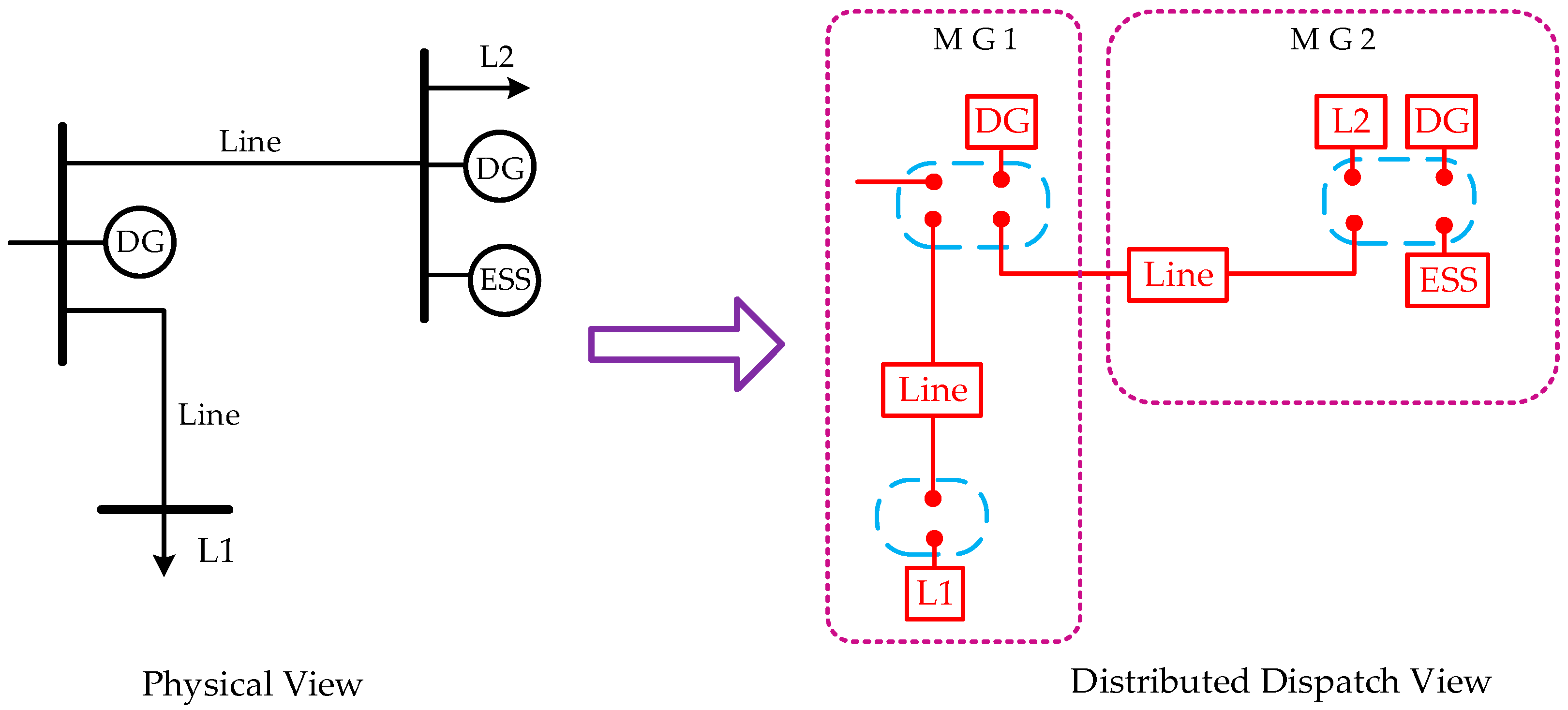
3.1. Decomposition of a Networked Microgrid (NM)

An NM can be seen as a variety of components with terminals that could be aggregated into multiple entities. As demonstrated in Figure 1, NMs are thus modeled as networked entities. A junction is made of a set of terminals associated with the same bus.

Define N as a finite set of microgrids, J as a finite set of coupled junctions, and M as a finite set of terminals, of which the cardinality is divided into subsets according to microgrid a or junction j. Each terminal represents an abstract electric variable, such as complex power or voltage magnitude. S_m and V_m, respectively, represent the complex power and voltage magnitude of terminal m. The set of complex power and voltage magnitude associated with microgrid a are represented by S_a = {S_m|m $\in$ a} and V_a = {V_m|m $\in$ a}, respectively. Here, if microgrid a has one terminal, then S_a is a vector and V_a is a scalar. By the same token, the set of complex power and voltage magnitude associated with junction j are respectively denoted by S_j = {S_m|m $\in$ j} and V_j = {V_m|m $\in$ j}.

During each time slot, the network must maintain power balance and voltage-magnitude consistency at each junction. Thereby, average net power imbalance ${\overline{S}}_m$ and voltage-magnitude residual are defined as:

$${\overline{S}}_m=\frac{1}{\left|j\right|}{\displaystyle \sum _{m\in j}{S}_m}$$

(16)

$${\tilde{V}}_m=V_m-\frac{1}{\left|j\right|}{\displaystyle \sum _{m\in j}{V}_m}=V_m-{\overline{V}}_m$$

(17)

Hence, the optimization model can be formulated as:

$$\left(\mathrm{F}1\right)\min {\displaystyle \sum _{a\in \mathrm{N}}{F}_a(S_a,V_a)}$$

(18)

$$s.t.\overline{S}=0,\tilde{V}=0$$

(19)

$$S\in \mathbf{S}\mathrm{and}V\in \mathbf{V}$$

(20)

where S and V, respectively, represent the decomposable constraints of S and V.

3.2. ADMM Algorithm

ADMM is attracting increasing attention from academic researchers primarily due to its decomposability along with superior convergence properties. Specifically, ADMM can solve a special form of optimization problems [35], as described by:

$$\min f(x)+g(z)$$

(21)

$$s.t.x-z=0$$

(22)

where $x$ belongs to a convex set and z is a dummy variable corresponding to x, and $g(z)$ is an indicator function. The augmented Lagrangian is formed as:

$$L_{\rho }(x,z,y)=f(x)+g(z)+y^T(x-z)+(\rho /2){\Vert x-z\Vert }_2^2$$

(23)

where $\rho$ is the step size. Next, a scale form of the augmented Lagrangian is derived, which gives a more concise formulation of the iteration process. Scaling multiplier $y$ to $u=y/\rho$ and combining linear and quadratic terms in the augmented Lagrangian function yield

$$y^T(x-z)+(\rho /2){\Vert x-z\Vert }_2^2=(\rho /2){\Vert x-z+y/\rho \Vert }_2^2-(1/2\rho ){\Vert y\Vert }_2^2=(\rho /2){\Vert x-z+u\Vert }_2^2-(1/2\rho ){\Vert y\Vert }_2^2$$

(24)

Using the scaled dual variables, ADMM comprises the following iterations:

$$\{\begin{array}{l}{x}^{k+1}:=\underset{x}{\arg \min }\left(f(x)+(\rho /2){\Vert x-z^k+u^k\Vert }_2^2\right)\\ z^{k+1}:=\underset{z}{\arg \min }\left(g(z)+(\rho /2){\Vert x^{k+1}-z+u^k\Vert }_2^2\right)\\ u^{k+1}:=u^k+x^{k+1}-z^{k+1}\end{array}$$

(25)

Accordingly, (F1) can be reformulated into the ADMM form as:

$$\left(\mathrm{F}2\right)\min {\displaystyle \sum _{a\in \mathbf{N}}{F}_a(S_a,V_a)}+{\displaystyle \sum _{j\in \mathbf{J}}[g_j({\eta }_j)+h_j({\zeta }_j)]}$$

(26)

$$S=\eta (y_P),V=\zeta (y_v)$$

(27)

$$S\in \mathbf{S}\mathrm{and}V\in \mathbf{V}$$

(28)

where $g_j({\eta }_j)$ and $h_j({\zeta }_j)$ are the indicator functions as defined below, while $\eta$ and $\zeta$ are dummy variables:

$$g_j({\eta }_j)=\{\begin{array}{ll}0& {\eta }_j\in \left\{{\eta }_j\right|{\overline{\eta }}_j=0\}\\ +\infty & {\eta }_j\notin \left\{{\eta }_j\right|{\overline{\eta }}_j=0\}\end{array}$$

(29)

$$h_j({\zeta }_j)=\{\begin{array}{ll}0& {\zeta }_j\in \left\{{\zeta }_j\right|{\tilde{\zeta }}_j=0\}\\ +\infty & {\zeta }_j\notin \left\{{\zeta }_j\right|{\tilde{\zeta }}_j=0\}\end{array}$$

(30)

Dual variables are scaled to $u=y_P/\rho$ and $u=y_v/\rho$. The augmented Lagrangian function for (F2) is then formulated as:

$$L_{\rho }^{F2}={\displaystyle \sum _{a\in \mathbf{N}}{F}_a(S_a,V_a)}+{\displaystyle \sum _{j\in \mathbf{J}}[g_j({\eta }_j)+h_j({\zeta }_j)]}+(\rho /2)({\Vert S-\eta +u\Vert }_2^2+{\Vert V-\zeta +n\Vert }_2^2)$$

(31)

Similarly, the iteration process comprises the following three steps:

$$(S_a^{k+1},V_a^{k+1}):=\underset{S_a,V_a}{\arg \min }(F_a(S_a,V_a)+(\rho /2)\ast ({\Vert S_a-{\eta }_a^k+u_a^k\Vert }_2^2+{\Vert V_a-{\zeta }_a^k+n_a^k\Vert }_2^2))a\in \mathbf{N}$$

(32)

$$\{\begin{array}{l}{\eta }_j^{k+1}:=\underset{{\eta }_j}{\arg \min }(g_j({\eta }_j)+(\rho /2)\ast ({\Vert S_j^{k+1}-{\eta }_j^{}+u_j^k\Vert }_2^2))j\in \mathbf{J}\\ {\zeta }_j^{k+1}:=\underset{{\zeta }_j}{\arg \min }(h_j({\zeta }_j)+(\rho /2)\ast ({\Vert V_j^{k+1}-{\zeta }_j^{}+n_j^k\Vert }_2^2))j\in \mathbf{J}\end{array}$$

(33)

$$\{\begin{array}{ll}{u}_j^{k+1}:=S_j^{k+1}-{\eta }_j^{k+1}& j\in \mathbf{J}\\ n_j^{k+1}:=V_j^{k+1}-{\zeta }_j^{k+1}& j\in \mathbf{J}\end{array}$$

(34)

The first step shown in Equation (31) is carried out, in parallel, by all devices, while the second and third steps shown in Equations (32)–(33) are implemented in parallel by all local controllers at each junction [36]. Since $g_j({\eta }_j)$ and $h_j({\zeta }_j)$ are simple indicator functions, a closed-form solution for the second step is thus derived and given by:

$$\{\begin{array}{l}{\eta }_j^{k+1}:=u_j^k+S_j^{k+1}-{\overline{u}}_j^k+{\overline{S}}_j^{k+1}\\ {\zeta }_j^{k+1}:={\overline{V}}_j^{k+1}+{\overline{n}}_j^k\end{array}$$

(35)

Subsisting Equation (35) into the first step (32) and third step (34), and then eliminating artificial variables $\eta$ and $\zeta$, a simplified iteration process is attained, as illustrated in Algorithm 1.

Algorithm 1. Modified Alternating-Direction Multiplier Method (ADMM) algorithm.

1. State variables update

$(S_a^{k+1},V_a^{k+1}):=\underset{S_a,V_a}{\arg \min }(F_a(S_a,V_a)+(\rho /2)\times ({\Vert S_a-S_a^k+{\overline{S}}_a^k+u_a^k\Vert }_2^2+{\Vert V_a-{\overline{V}}_a^k-{\overline{n}}_a^{k-1}+n_a^k\Vert }_2^2))a\in \mathbf{N}$

2. Dual variables update

$\begin{array}{cc}{u}_j^{k+1}:={\overline{u}}_j^k+{\overline{S}}_j^{k+1}& j\in \mathbf{J}\\ n_j^{k+1}:={\tilde{n}}_j^k+{\tilde{V}}_j^{k+1}& j\in \mathbf{J}\end{array}$

3.3. Overall Solution Framework

As the proposed solution method represents a version of ADMM and the established model is convex, this method can guarantee a global optimal solution to be attained. To determine the termination criterion, two types of residuals [35], i.e., primal and dual, are introduced and denoted by r^k and s^k for the k-th iteration, as formulated by:

$$r^k=({\overline{S}}^k,{\tilde{V}}^k)$$

(36)

$$s^k=\rho ((S^k-{\overline{S}}^k)-(S^{k-1}-{\overline{S}}^{k-1}),{\overline{V}}^k-{\overline{V}}^{k-1})$$

(37)

The following criteria are defined for checking convergence:

$${\Vert r^k\Vert }_2\le e^{pri}\mathrm{and}{\Vert s^k\Vert }_2\le e^{dual}$$

(38)

where e^pri and e^dual represent primal and dual tolerances, respectively. These tolerances should be normalized to the absolute tolerance e^abs according to network size, defined as:

$$e^{abs}=e^{pri}/\sqrt{\left|\mathbf{M}\right|\times T}=e^{dual}/\sqrt{\left|\mathbf{M}\right|\times T}$$

(39)

where |M| is the total number of terminals in an NM. This solving process is illustrated in Figure 2.

An inappropriate step-size value may profoundly affect solving speed and even cause the solving procedure to diverge. Thus, it is of importance to choose an optimal step size. Here, a variable step-size scheme [35] is employed. In other words, step size $\rho$ is variable in the iteration procedure so as to enhance convergence speed as well as avoid the negative impact of the initial value on attaining good convergence performance. A commonly used updating mechanism is given as:

$${\rho }^{k+1}:=\{\begin{array}{ll}\tau {\rho }^k& if{\Vert r^k\Vert }_2>\mu {\Vert s^k\Vert }_2\\ {\rho }^k/\tau & if{\Vert r^k\Vert }_2<\mu {\Vert s^k\Vert }_2\\ {\rho }^k& \mathrm{otherwise}\end{array}$$

(40)

where $\mu >1$, $\tau >1$. Here, $\mu$ and $\tau$ are set as 20 and 2, respectively.

As for the NM dispatch framework, the (k + 1) th iteration of optimization model for microgrid a is formulated as follows:

$$\begin{array}{l}\min {\displaystyle {\sum }_{a\in \mathbf{N}}{\displaystyle {\sum }_{t\in \mathbf{T}}\left[{\displaystyle {\sum }_{d\in {\mathbf{N}}_a^G}f(P_{d,t}^{G,a})}+{\lambda }_t^{}{P}_{a,t}^M+{\displaystyle {\sum }_{d\in {\mathbf{N}}_a^R}{\lambda }_t^{RES}{\overline{P}}_{d,t}^{RES}}\right]}}\\ \hspace{1em}\hspace{1em}\hspace{1em}\hspace{1em}\hspace{1em}\hspace{1em}\hspace{1em}\hspace{1em}\hspace{1em}\hspace{1em}\hspace{1em}\hspace{1em}\hspace{1em}\hspace{1em}\hspace{1em}\hspace{1em}\hspace{1em}\hspace{1em}\hspace{1em}+(\frac{\rho }{2})\times ({\Vert S_a-S_a^k+{\overline{S}}_a^k+u_a^k\Vert }_2^2+{\Vert v_a-{\overline{v}}_a^k-{\overline{n}}_a^{k-1}+n_a^k\Vert }_2^2))\end{array}$$

(41)

$$s.t.\left(4\right)-\left(14\right)$$

(42)

So far, an SOC problem is obtained, and can be solved by off-the-shell solvers. Note that the proposed ADMM-based method solves the presented optimization model in a fully distributed manner with limited information exchange among neighboring microgrids. Specifically, each microgrid exchanges its present primal solution with its neighboring microgrids at every iteration. In each microgrid, the dual variables are updated, and the convergence criterion is checked. If the convergence criterion is met, the process is terminated. Otherwise, the iteration continues.

4. Case Studies

In this section, the presented model and method were tested on a modified IEEE 33-bus distribution system. Numerical experiments were carried out with MATLAB 2014 (MathWorks, Inc., Natick, MA, USA) on a laptop with an Intel Core (i5, 3.20 GHz) and 8 GB memory. MOSEK 7.0 [37] was invoked to solve the SOC problem.

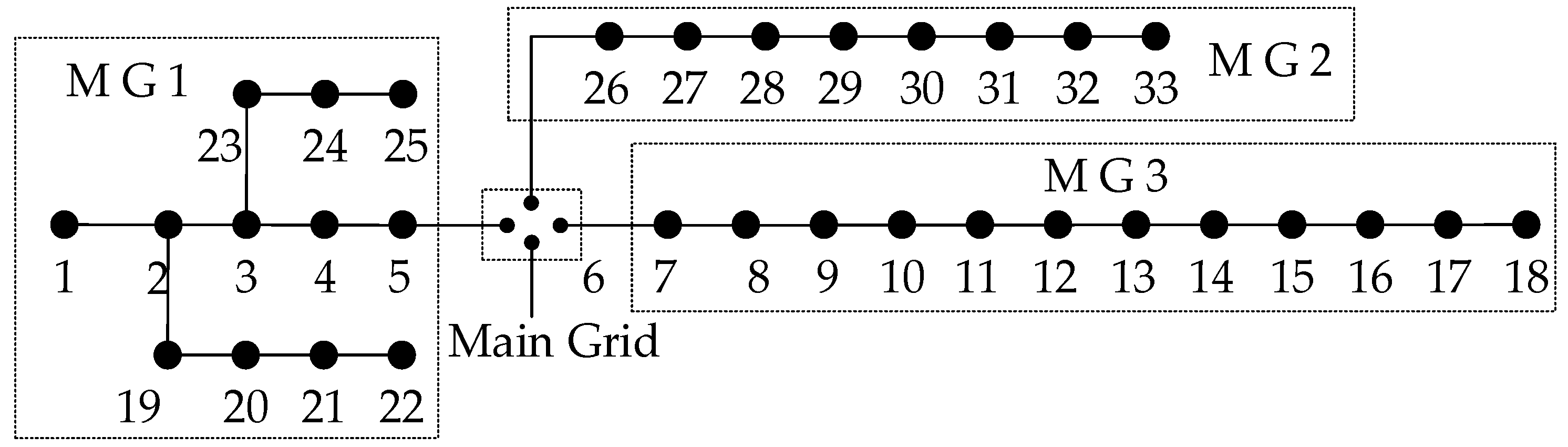
4.1. Simulation Data

The original system data are available in Reference [10]. The test system was partitioned into three microgrids, as shown in Figure 3. Bus 6, with a voltage magnitude of 1.05 p.u., was connected to the main grid. It was assumed that four fuel-based DGs were connected to buses 4, 17, 23, and 32, respectively. The pertinent data for fuel-based DGs are given as follows: fuel-based DG $d\in {\mathbf{N}}_a^G$, $f(P_{d,t}^{G,a})=0.07\times {(P_{d,t}^{G,a})}^2+0.1\times P_{d,t}^{G,a}$, ${\gamma }^{G,\max }=5\mathrm{kW}/\mathrm{h}$, ${\underset{\_}{P}}_d^G=0\mathrm{kW}$, and ${\overline{P}}_d^G=20\mathrm{kW}$.

Electricity-price data adapted from Pennsylvania—New Jersey—Maryland (PJM) electricity market are presented in Figure 4a. The renewable energy-generated electricity price was set at 30 $/MWh. Given that photovoltaic is the dominant RES-based DG in a real-life medium-voltage distribution system, it is assumed that there are six photovoltaic systems installed at buses 3, 12, 16, 20, 23, and 27. The solar-irradiation data were collected on January 16, 2016 at the University of Queensland [38], lasting from 5:00 to 18:00. It is assumed that all installed photovoltaics are geographically close to each other, and, thus, the same solar-irradiance data are applied in case studies. The capacity of all photovoltaics was set as 100 kVA and nominal power factors were set as 0.95. The nodal-voltage magnitudes were maintained within the prespecified interval of [0.95, 1.05] during the entire optimization horizon. The proposed model was used to mitigate voltage violations from occurrence as a variable photovoltaic power output and a fuel-based DG power output were utilized.

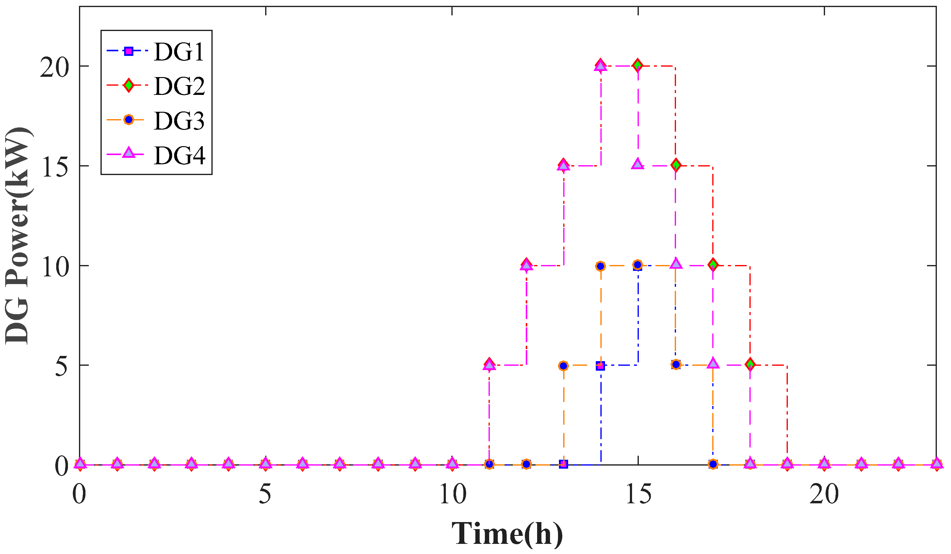
4.2. Optimization Results

Figure 5 illustrates the power procurement from the main grid for three microgrids, and Figure 6 demonstrates nodal-voltage magnitudes at representative buses—3, 16, and 30. Energy procurements for the three microgrids increased during peak load hours (i.e., 11:00–20:00), which corresponded to significant voltage drops at the selected buses. Note that there was a sharp drop of voltage magnitude at bus 16 during 14:00–15:00. This is mainly because the photovoltaic output power at bus 16 substantially decreased at the corresponding period. Similarly, there was a slight increase of voltage magnitude at bus 16 during 22:00–23:00, and photovoltaic output power at the same bus went up correspondingly.

Figure 7 shows that fuel-based DGs would operate during energy-price peak periods because less energy was bought from the main grid at higher prices. DGs at buses 17 and 32 would operate at 11:00, while DGs at buses 4 and 23 within microgrid 1 started up at 13:00 and 14:00, respectively. This is reasonable because the locational marginal prices at buses 17 and 32 (more remote from the slack bus) were comparatively higher than those at buses 4 and 23, primarily due to network loss and voltage-magnitude limit. Once the locational marginal price was higher than the average cost of fuel-based DGs, the operator would rather increase the output power of fuel-based DGs. Thus, as shown in Figure 8, the DGs at buses 17 and 32 worked for more periods than DGs at buses 4 and 23.

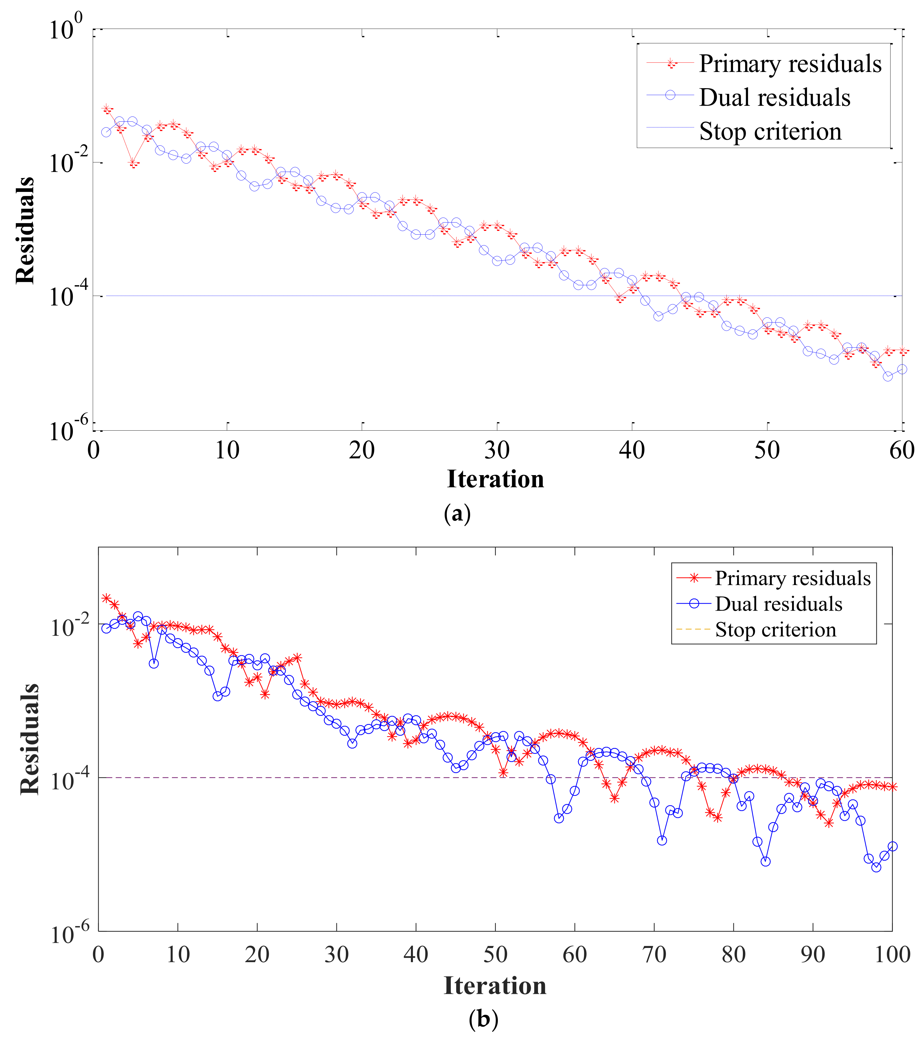
4.3. Convergence Analysis

Note that all case studies were implemented on the same computer. Hence, in order to estimate the calculation time when the solving method was run in a parallel fashion, the most time-consuming microgrid was selected to evaluate the speed of the proposed algorithm in case studies. Thereby, time latency was neglected since it was assumed that bandwidth could accommodate the communication needs of the proposed strategy.

The termination criterion, e^abs, was set as 10⁻⁴. When the primary and dual residuals were both less than the termination criterion, the computation procedure was completed. In case studies, the proposed ADMM algorithm converged in 43 iterations, as shown in Figure 8a, and consumed 3.44 s. The IEEE 123 bus test system was employed to conduct sensitivity analysis in terms of problem size. Note that the network was divided into six control entities and the network partition strategy, along with photovoltaic settings, were the same as those in Reference [3]. As shown in Figure 8b, the proposed algorithm converged in 85 iterations and consumed 6.60 s. As can be seen from numerical results, the iteration number of the proposed method for the IEEE 123 bus test system was still acceptable, and this demonstrates that the proposed method could effectively accommodate a variety of microgrids and be robust against the network size. Calculation time for the two test systems demonstrated that the proposed method is applicable even in a real-time market environment.

Two step-size schemes, i.e., variable and fixed, were employed in the case studies to highlight the advantages of the variable step-size scheme. As shown in

Table 1. Comparison between two modes.

Initial Value $\rho$	0.01	0.1	0.5	1	10	100
Fixed-$\rho$	623	73	42	50	Divergence	Divergence
Variable-$\rho$	40	50	43	53	64	59

, when the initial value of the step size was set as 10 or 100, only the variable step-size scheme could achieve a global optimum, while the fixed one was infeasible. Moreover, when the step size was specified as small as 0.01, more iterations were demanded for the fixed step-size scheme than the variable one. Hence, the variable step-size scheme was more robust with respect to the choice of the initial step-size value, and was, thereby, more practical in engineering applications.

The robustness of the proposed method was examined under given communication failure. Specifically, it was supposed that a random malfunction of the communication system occurred during the solving process and, hence, interrupted information exchange processes. The malfunction was modeled as random packet drops. More formally, each microgrid operator might fail to obtain information from neighboring microgrids with a certain probability. Thereby, it is assumed that the microgrid operator would employ the information attained in the last iteration if malfunctions occurred. As can be seen in

Table 2. Robustness performance.

Probability	0.1	0.2	0.3
Required iteration number	44	51	60

, the proposed method can guarantee an optimal solution even when a random packet drop occurs. More specifically, more iterations would be needed if the probability of communication failure increased. Besides, it is also demonstrated that the proposed control strategy is capable of accommodating frequent changes in system-operating conditions as a result of extensive penetrations of plug-and-play devices. For example, the microgrid operator could immediately detect the related power consumption/injection when a number of plug-in electric vehicles were integrated into a microgrid, and then send the information to its neighbors at the next iteration, without terminating the solving process.

4.4. Accuracy of Second-Order Cone (SOC) Relaxation

To examine whether the developed SOC relaxation was exact, it was necessary to check whether Inequality (14) was binding at the optimal solution. Hence, the evaluation index is defined as:

$$de{v}_t={\Vert {\ell }_{ik,t}^{}-\frac{{\left(P_{ik,t}^{}\right)}^2+{\left(Q_{ik,t}^{}\right)}^2}{v_{i,t}^{}}\Vert }_{\infty }$$

(43)

where dev_t denotes the maximum residual of the square of the current magnitude in all distribution branches. Evaluation results are shown in Figure 9, wherein the defined evaluation index for the whole optimization horizon was less than 10⁻⁶. More importantly, it was remarkably less than the square of the current magnitude. Therefore, the SOC-relaxation technique can offer a theoretically optimal solution with high computation speed.

5. Conclusions

In this work, a new distributed energy-management optimization model was developed to ensure secure and economic operation of an NM. The conic-relaxation technique was employed to convexify the optimization model into an SOC model. Then, an ADMM-based distributed algorithm was developed to solve the attained convex problem, with only broadcasting and gathering limited messages among neighboring microgrids required. The proposed method could accommodate a variety of DGs, and has good convergence and fast solving speed, as demonstrated by case studies. The advantages of the proposed method are twofold: (1) the developed optimization model can accommodate the ever-increasing integration of controllable DGs, and is capable of coordinating a variety of DGs in a distributed fashion; (2) the developed distributed method can mitigate the risk of exposing the privacy of customers, since the controller in each microgrid only requires limited information from its neighboring microgrids.

The branch-flow model and SOC relaxation in this work are only applicable for radial networks. In our future research efforts, the presented model in this work will be extended to meshed networks.

References

1. Ilic, M. From hierarchical to open access electric power systems. Proc. IEEE 2007, 95, 1060–1084. [Google Scholar] [CrossRef]
2. Wang, Z.; Chen, B.; Wang, J.; Kim, J. Decentralized energy management system for networked microgrids in grid-connected and islanded modes. IEEE Trans. Smart Grid 2016, 7, 1097–1105. [Google Scholar] [CrossRef]
3. Feng, C.; Li, Z.; Shahidehpour, M.; Wen, F.; Liu, W.; Wang, X. Decentralized short-term voltage control in active power distribution systems. IEEE Trans. Smart Grid 2018, 5, 4566–4576. [Google Scholar] [CrossRef]
4. Li, Z.; Shahidehpour, M.; Wu, W.; Zeng, B.; Zhang, B.; Zheng, W. Decentralized multiarea robust generation unit and tie-lie scheduling under wind power uncertainty. IEEE Trans. Sustain. Energy 2015, 6, 1377–1388. [Google Scholar] [CrossRef]
5. Mashhour, E.; MOghaddas-Tafreshi, S. Bidding strategy of virtual power plant for participating in energy and spinning reserve markets-Part I: Problem formulation. IEEE Trans. Power Syst. 2011, 2, 949–956. [Google Scholar] [CrossRef]
6. Mao, M.; Jin, P.; Hatziagyriou, N.D.; Chang, L. Multiagent-based hybrid energy management system for microgrids. IEEE Trans. Sustain. Energy 2014, 5, 938–946. [Google Scholar] [CrossRef]
7. Jiang, Q.; Xue, M.; Geng, G. Energy management of microgrid in grid-connected and stand-alone modes. IEEE Trans. Power Syst. 2013, 28, 3380–3389. [Google Scholar] [CrossRef]
8. Chung, H.; Li, W.; Yuen, C.; Wen, C.; Crespi, N. Electric vehicle charge scheduling mechanism to maximize cost efficiency and user convenience. IEEE Trans. Smart Grid 2018. [Google Scholar] [CrossRef]
9. Margellos, K.; Oren, S. Capacity controlled demand side management: A stochastic pricing analysis. IEEE Trans. Power Syst. 2016, 31, 706–717. [Google Scholar] [CrossRef]
10. Qi, F.; Wen, F.; Liu, X.; Salam, M. A residential energy hub model with a concentrating solar power plant and electric vehicles. Energies 2017, 10, 1159. [Google Scholar] [CrossRef]
11. Wang, Y.; Wang, B.; Chu, C.; Pota, H.; Gadh, R. Energy management for a commercial building microgrid with stationary and mobile battery storage. Energy Build. 2016, 116, 141–150. [Google Scholar] [CrossRef] [Green Version]
12. Conejo, A.J.; Castillo, E.; Minguez, R. Decomposition Techniques in Mathematical Programming: Engineering and Science Applications; Springer: Berlin, Germany, 2006; Volume 2, pp. 187–239. ISBN 9783540276869. [Google Scholar]
13. Cohen, G. Auxiliary problem principle and decomposition of optimization problems. J. Optim. Theory Appl. 1980, 32, 277–305. [Google Scholar] [CrossRef]
14. Kim, B.H.; Baldick, R. Coarse-grained distributed optimal power flow. IEEE Trans. Power Syst. 1997, 12, 932–939. [Google Scholar] [CrossRef]
15. Mohammadi, A.; Megrtash, M.; Kargarian, A. Diagonal quadratic approximation for decentralized collaborative TSO+DSO optimal power flow. IEEE Trans. Smart Grid 2018. [Google Scholar] [CrossRef]
16. Conejo, A.J.; Nogales, F.J.; Prieto, F.J. A decomposition procedure based on approximate Newton directions. Math. Program 2002, 93, 495–515. [Google Scholar] [CrossRef] [Green Version]
17. Li, Z.; Guo, Q.; Sun, H.; Wang, J. Coordinated economic dispatch of coupled transmission and distributed systems using heterogeneous decomposition. IEEE Trans. Power Syst. 2016, 31, 4817–4830. [Google Scholar] [CrossRef]
18. Guo, J.; Hug, G.; Tonguz, O.K. Intelligent partitioning in distributed optimization of electric power systems. IEEE Trans. Smart Grid 2016, 7, 1249–1258. [Google Scholar] [CrossRef]
19. Li, J.; Xu, Z.; Wang, J.; Zhao, J.; Zhang, Y. Distributed transactive energy trading framework in distribution networks. IEEE Trans. Smart Grid 2018. [Google Scholar] [CrossRef]
20. Liu, Y.; Gooi, H.; Jian, H.; Xin, H. Distributed robust energy management of a multi-microgrid system in the real-time energy market. IEEE Trans. Sustain. Energy 2017. [Google Scholar] [CrossRef]
21. Tanaka, K.; Oshiro, M.; Toma, S.; Yona, A.; Senjyu, T.; Funabashi, T.; Kim, C.H. Decentralized control of voltage in distribution systems by distributed generators. IET Gener. Transm. Distrib. 2010, 4, 1251–1260. [Google Scholar] [CrossRef]
22. Gan, L.; Low, S.H. Convex relaxations and linear approximation for optimal power flow in multiphase radial network. In Proceedings of the 18th Power Systems Computation Conference (PSCC), Wroclaw, Poland, 18–22 August 2014; pp. 1–9. [Google Scholar] [CrossRef]
23. Peng, Q.; Low, S.H. Distributed algorithm for optimal power flow on a radial network, I: Balanced single-phase case. IEEE Trans. Smart Grid 2018, 9, 111–121. [Google Scholar] [CrossRef]
24. Low, S.H. Convex relaxation of optimal power flow Part I: Formulations and equivalence. IEEE Trans. Control Netw. Syst. 2014, 1, 15–27. [Google Scholar] [CrossRef]
25. Farivar, M.; Neal, R.; Clarke, C.; Low, S.H. Optimal inverter VAR control in distribution systems with high PV penetration. In Proceedings of the IEEE Power and Energy Society General Meeting, San Diego, CA, USA, 23–26 July 2012; pp. 1–6. [Google Scholar] [CrossRef]
26. Li, N.; Chen, L.; Low, S.H. Exact convex relaxation of optimal power flow for radial networks using branch flow model. IEEE Trans. Autom. Control 2012, 60, 72–87. [Google Scholar] [CrossRef]
27. Wang, Q.; Zhang, C.; Di, Y.; Xydis, G.; Wang, J.; Østergaad, J. Review of real-time electricity markets for integrating distributed energy resources and demand response. Appl. Energy 2015, 138, 695–706. [Google Scholar] [CrossRef]
28. Hu, J.; Wen, F.; Wang, K.; Huang, Y.; Salam, M. Simultaneous provision of flexible ramping product and demand relief by interruptible loads considering economic incentives. Energies 2018, 11, 46. [Google Scholar] [CrossRef]
29. Tsikalakis, A.G.; Hatziargyriou, N.D. Centralized control for optimizing microgrids operation. IEEE Trans. Energy Convers. 2008, 23, 241–248. [Google Scholar] [CrossRef]
30. Shen, J.; Jiang, C.; Liu, Y.; Wang, X. A microgrid energy management system and risk management under an electricity market environment. IEEE Access 2016, 4, 2349–2356. [Google Scholar] [CrossRef]
31. Rahimiyan, M.; Baringo, L.; Conejo, A.J. Energy management of a cluster of interconnected price-responsive demands. IEEE Trans. Power Syst. 2014, 29, 645–655. [Google Scholar] [CrossRef]
32. Nguyen, D.T.; Le, L.B. Risk-constrained profit maximization for microgrid aggregators with demand response. IEEE Trans. Smart Grid 2015, 6, 135–146. [Google Scholar] [CrossRef]
33. Malepor, A.R.; Anil, P.; Sanjoy, D. Inverter-based VAR control in low voltage distribution systems with rooftop solar PV. In Proceedings of the IEEE North American Power Symposium (NAPS), Manhattan, KS, USA, 22–24 September 2013; pp. 1–5. [Google Scholar] [CrossRef]
34. American National Standard for Electric Power Systems and Equipment—Voltage Ratings (60 Hertz); ANSI Standard C84.1-2006; National Electrical Manufacturers Association: Rosslyn, VA, USA, 2006.
35. Boyd, S.; Parikh, N.; Chu, E.; Peleato, B.; Eckstein, J. Distributed optimization and statistical learning via the alternating direction method of multipliers. Found. Trends Mach. Learn. 2010, 3, 1–122. [Google Scholar] [CrossRef]
36. Kraning, M.; Chu, E.; Javaei, J.; Boyd, S. Dynamic network energy management via proximal message passing. Found. Trends Mach. Learn. 2013, 1, 70–122. [Google Scholar] [CrossRef]
37. MOSEK. Available online: https://mosek.com (accessed on 20 May 2018).
38. UQ SQLAR PV Data. Available online: http://solar.uq.edu.au/ (accessed on 26 January 2016).
Figure 1. The distributed paradigm for a networked microgrid (NM).
Energies 11 02555 g001
Figure 2. Flowchart of the decentralized dispatch in an NM.
Energies 11 02555 g002
Figure 3. The single line graph of the NM.
Energies 11 02555 g003
Figure 4. (a) Energy price λ t ; (b) photovoltaic output power.
Energies 11 02555 g004
Figure 5. Energy procurement from the main grid for three microgrids.
Energies 11 02555 g005
Figure 6. Voltage magnitudes at the selected buses.
Energies 11 02555 g006
Figure 7. Power outputs of fuel-based distributed generators (DGs).
Energies 11 02555 g007
Figure 8. Iteration process. (a) IEEE 33 bus test system; (b) IEEE 123 bus test system.
Energies 11 02555 g008
Figure 9. Accuracy of second-order cone (SOC) relaxation.
Energies 11 02555 g009