A Distributed Randomized Gradient-Free Algorithm for the Non-Convex Economic Dispatch Problem

Abstract

In this paper, a distributed randomized gradient-free algorithm (DRGF) is employed to solve the complex non-convex economic dispatch problem whose non-convex constraints include valve-point loading effects, prohibited operating zones, and multiple fuel options. The DRGF uses the Gauss approximation, smoothing parameters, and a random sequence to construct distributed randomized gradient-free oracles. By employing a consensus procedure, generation units can gather local information through local communication links and then process the economic dispatch data in a distributed iteration format. Based on the principle of projection optimization, a projection operator is adopted in the DRGF to deal with the discontinuous solution space. The effectiveness of the proposed approach in addressing the non-convex economic dispatch problem is demonstrated by simulations implemented on three standard test systems.

1. Introduction

The general optimal economic dispatch is realized by designing unit commitment [1] for obtaining the minimum overall generation cost [2]. The centralized optimization methods are generally used in the economic dispatch problems, such as lambda iterative algorithms [3] and interior point algorithms [4], which require the objective function to be derivative. In practice, there exist conditions of valve-point loading effects in units’ startup stages [5], prohibited operating zones during the operation periods [6], and choices of the several economical fuels according to the actual power outputs [5]. These conditions make the economic dispatch problem non-convex, and in this paper, we investigate a non-convex optimization algorithm to address its non-convex characteristic.

Modern metaheuristic algorithms can solve non-convex optimization problems efficiently [7], mainly including genetic algorithm (GA [5,6,8]), particle swarm optimization (PSO [9,10,11,12]), differential evolution algorithms [13,14], and ant colony optimization (ACO, [15,16,17]). They all depend on dispatch centers to manage the information gathering from the whole system and will also use a centralized controller that will bring high communication costs. In addition, these controllers are prone to modeling errors and need a high-bandwidth communication structure with miscellaneous links [18]. Moreover, the reliability of the system is easily vulnerable to the single-point of failure [19]. Recently, the topology of power grids and communication networks are getting time-varying and extensible, but heuristic algorithms suffer a great challenge in meeting the changes.

At present, the distributed framework for economic dispatch has become a hot research topic [20,21,22]. Through building communication lines among the generation units and their neighbors, the distributed economic dispatch collects the essential iteration information and performs the real-time economic dispatch with global optimization. Simulations analyses in [20] show that the distributed dispatch will greatly cut down communication costs. The distributed gradient algorithm [21] has ensured the normal process of distributed economic dispatch when the events of units’ over-limits occur. It maintains the connectivity of the communication topology after reconstructing a virtual one. In [22], with the cost function of energy storage systems non-differentiable, the sub-gradient is used as an alternative of the gradient to implement the non-convex economic dispatch. The algorithms in [20,21,22] are not suitable for solving non-convex optimization problems for difficulties in calculating the cost function’s gradient or sub-gradient. The distributed auction-based algorithm (AA) proposed by [18] handles these non-convex constraints successfully through sharing bids among network agents and resolving the auction in a consensus procedure. However, it introduces too many intermediate variables, which will make the iteration format complex [23].

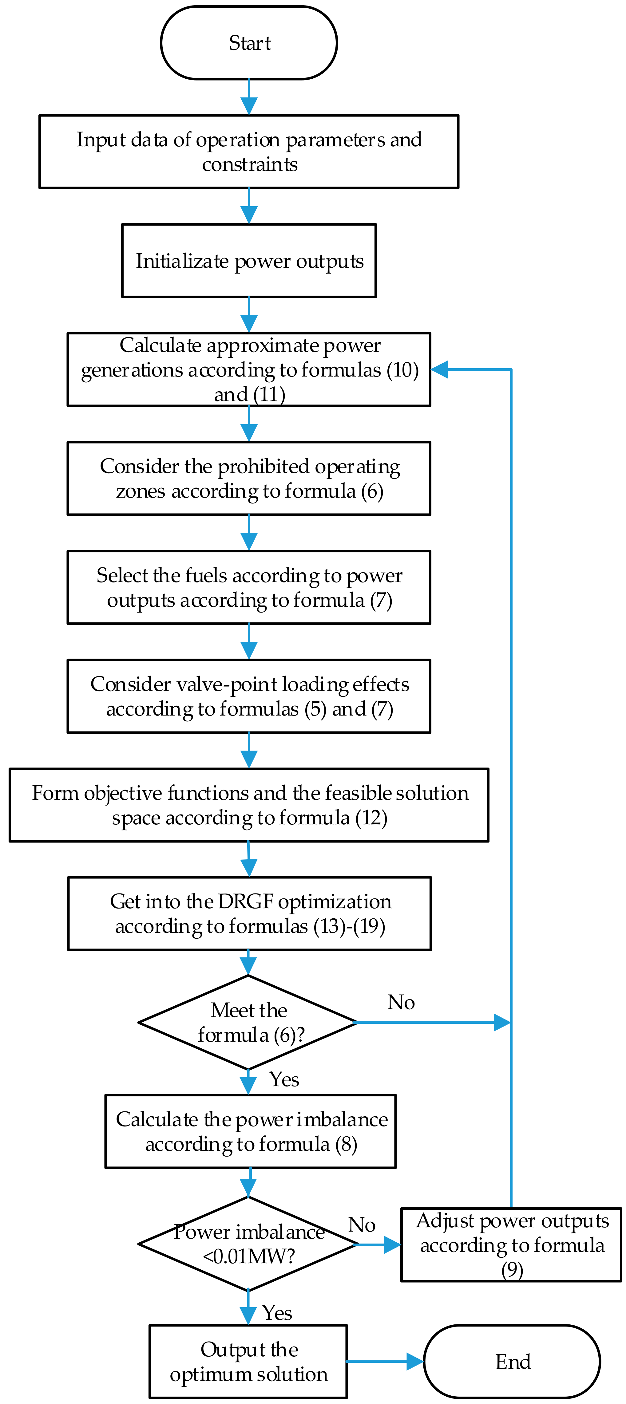
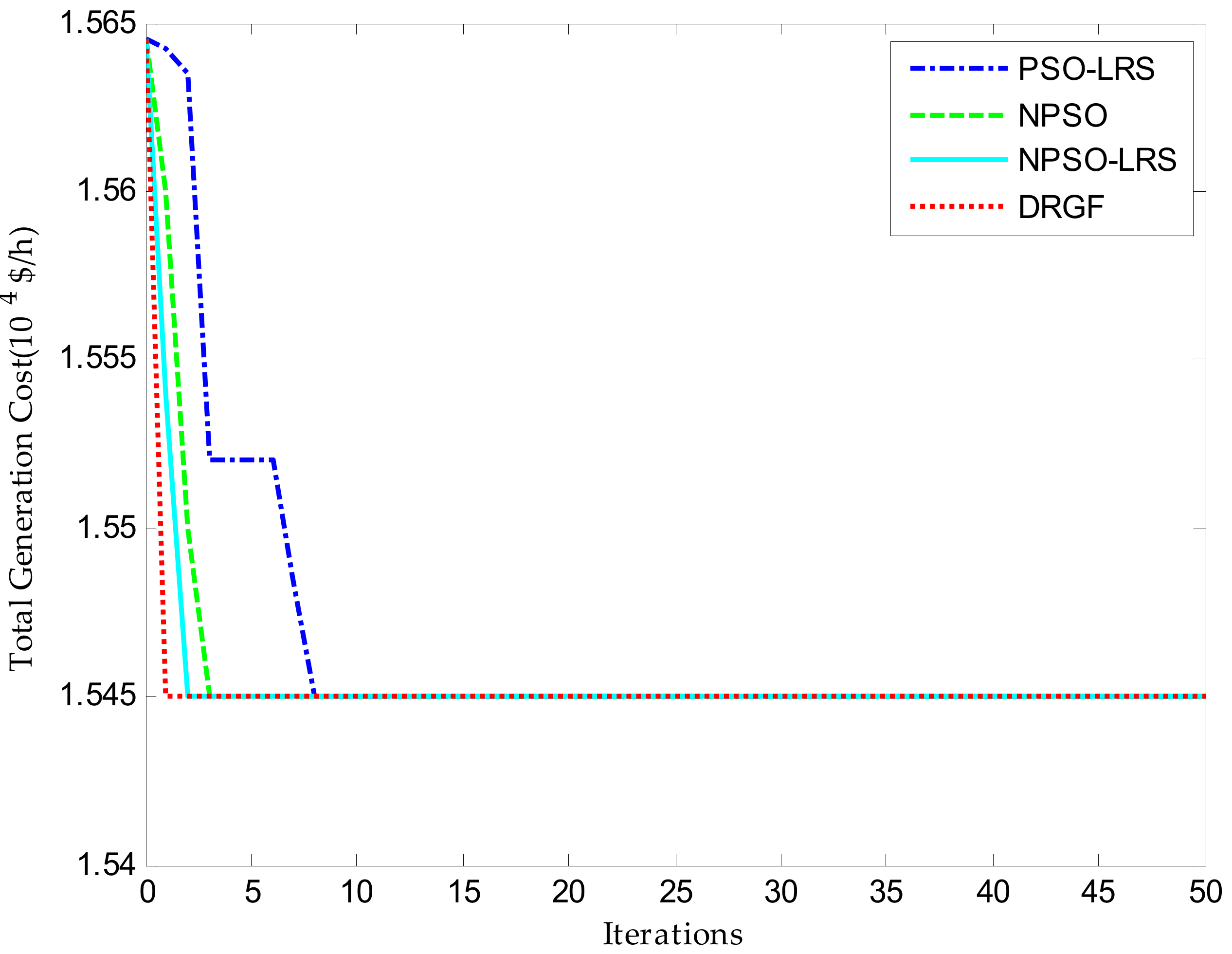
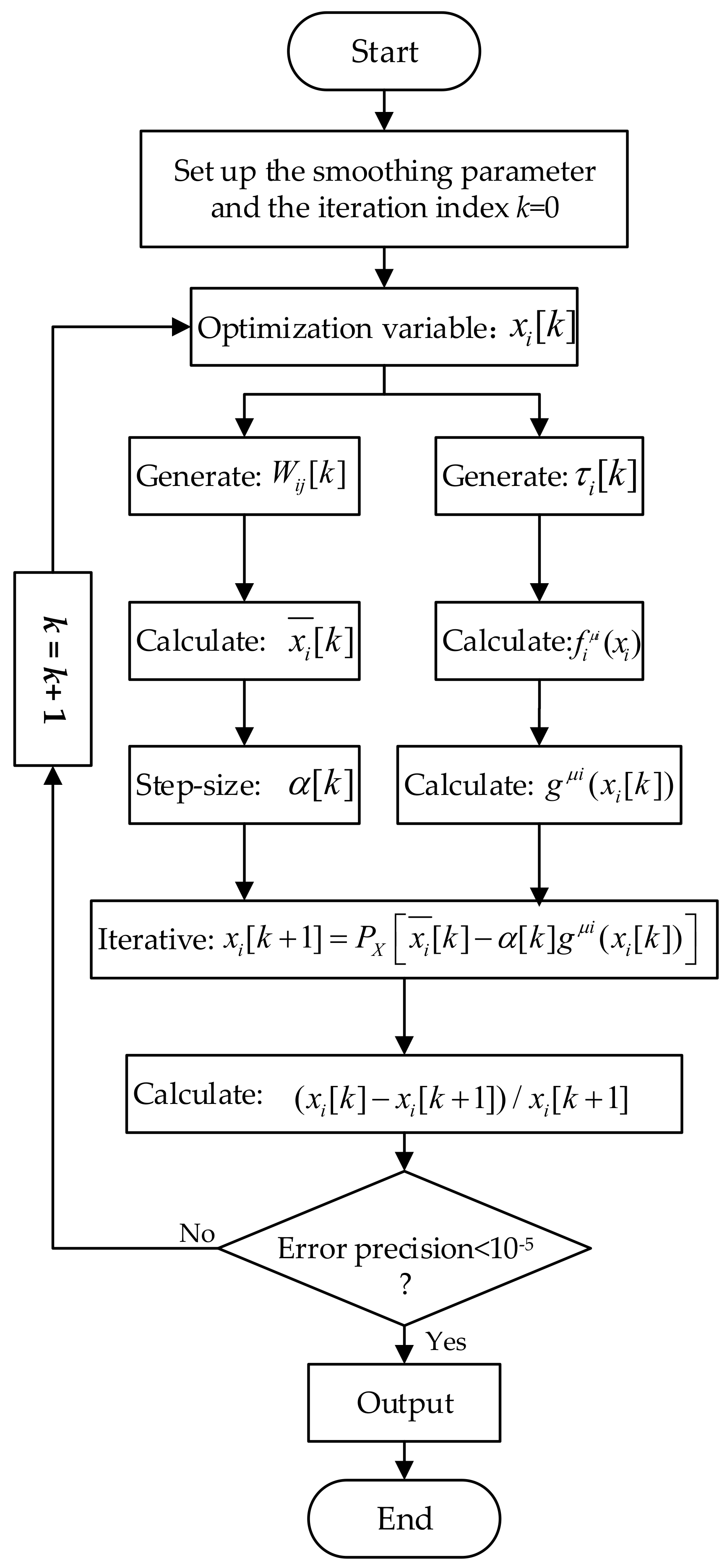
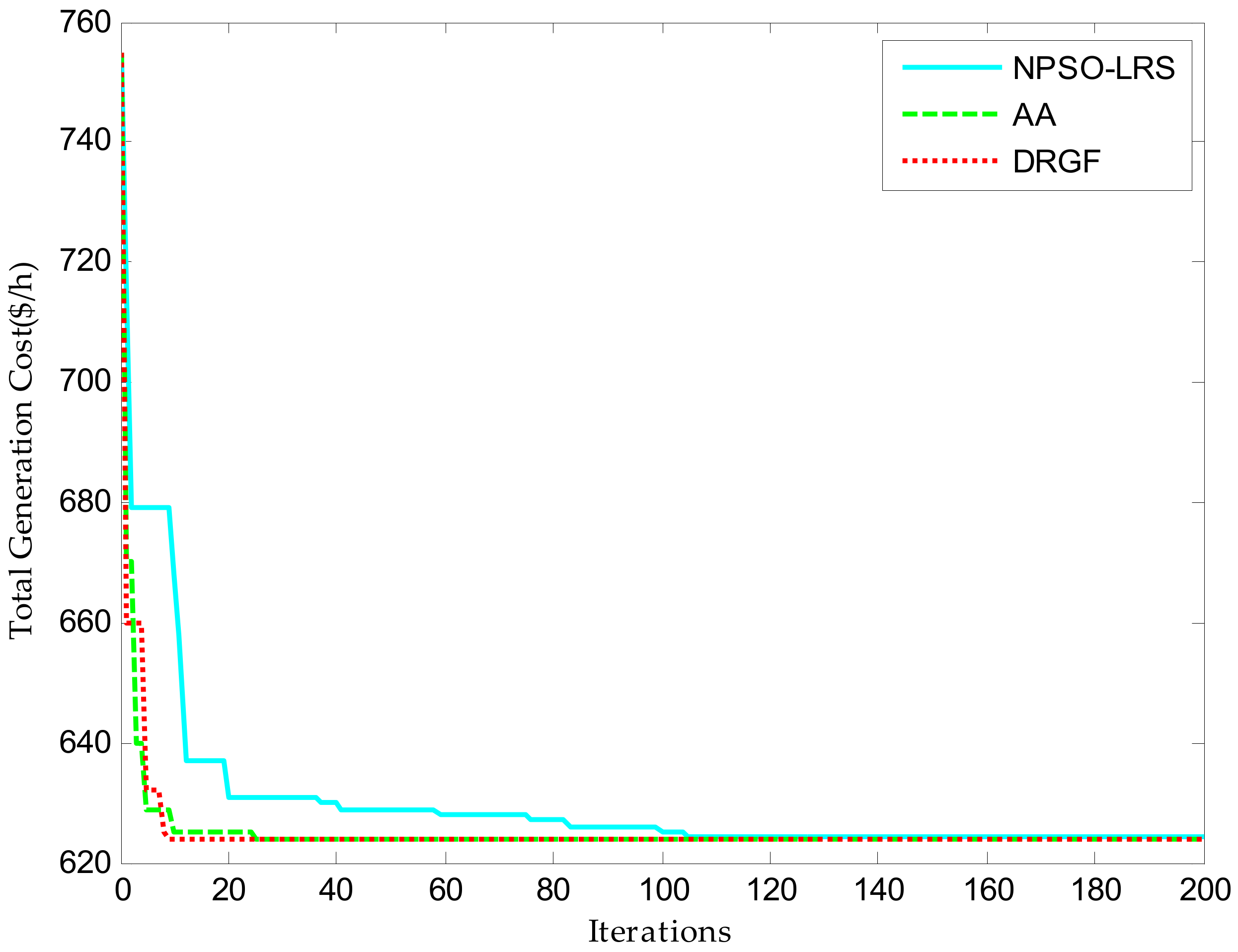
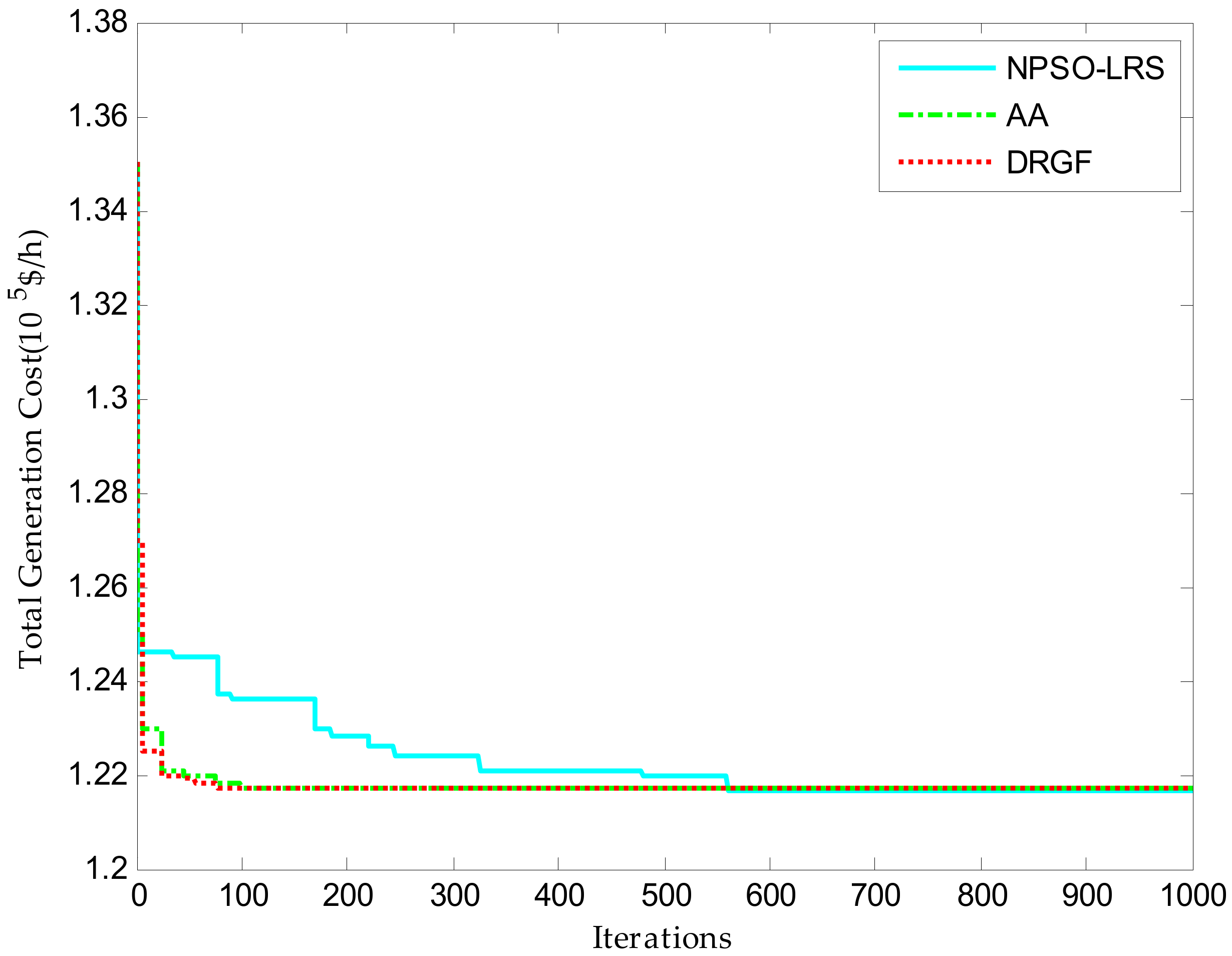
This paper adopts a distributed randomized gradient-free algorithm (DRGF) to solve non-convex economic dispatch problems with considering valve-point loading effects, prohibited operating zones, and multiple fuel options. The algorithm is based on a distributed communication structure which is cheap, reliable, and robust. Its iteration formula is implemented by employing the randomized derivative-free oracles. The effectiveness of the proposed method is verified on three test systems, and the simulation results indicate that the proposed DRGF approach can cope well with non-convex economic dispatch problems.

This paper is organized as follows. In Section 2, a non-convex economic dispatch with constraints of valve-point loading effects, prohibited operating zones, and multiple fuel options is presented. The DRGF is introduced in Section 3, and the simulation results presented in Section 4 show its effectiveness. Finally, the paper is concluded in Section 5.

2. Non-Convex Economic Dispatch

This paper studies an optimal loads allocation problem within a single time period. Under the premise of satisfying the system’s active power balance constraint and units’ power outputs limits, the total loads can be distributed among all of the units by a most economical scheme.

In conventional economic dispatch, the cost of a thermal generator unit is a quadratic function, and the dispatch center is aimed to minimize the total costs of all generation units.

$$\min C(P)={\displaystyle \sum _{i=1}^n{C}_i(P_i)}={\displaystyle \sum _{i=1}^n(a_i{P}_i{}^2+b_i{P}_i+c_i)}$$

(1)

where C(P) represents the total costs of all units whose total number is n; P_i is the power outputs of unit i and C_i(P_i) is the production cost. The production characteristic coefficients are a_i, b_i, and c_i.

If the ramp rate limits are considered, the power outputs limits can be expressed as [10]

$$\mathrm{Max}(P_i^{\min },P_i^o-D{R}_i)\le P_i\le \mathrm{Min}(P_i^{\max },P_i^o+U{P}_i)$$

(2)

where $P_i^o$ is the previous power output, the upper and lower power output limits are $P_i^{\max },P_i^{\min }$ respectively, and DR_i and UP_i are the down and up ramp limits, respectively.

The system must meet the active power balance constraints.

$${\displaystyle \sum _{i=1}^n{P}_i}=P_d+P_{loss}$$

(3)

where P_d is the total load demand. The network losses of the system are P_loss calculated by the Kron formula [18].

$$P_{loss}={\displaystyle \sum _{i=1}^n{\displaystyle \sum _{j=1}^n(P_i}}{B}_{ij}{P}_j)+{\displaystyle \sum _{i=1}^n(B_{0,i}{P}_i)+B_{00}}$$

(4)

where B_ij, B_0,i, and B₀₀ are the losses coefficients.

(a) Valve-point loading effects. To formulate the valve-point loading effects, a sinusoidal term is added to the original cost function [5]

$$C_i(P_i)=a_i{P}_i{}^2+b_i{P}_i+c_i+\left|d_i\sin (e_i{P}_i-e_i{P}_i^{\min })\right|$$

(5)

where d_i, e_i are the valve-point loading coefficients of unit i.

(b) Prohibited operating zones. Considering this constraint can ensure the stable operation of generation units. Therefore, the units’ power outputs constraints will be modified as follows [9]:

$$\{\begin{array}{l}\mathrm{M}ax(P_i^{\min },P_i^o-D{R}_i)\le P_i\le L_{m,i},\hspace{1em}m=1\hfill \\ U_{m-1,i}\le P_i\le L_{m,i},\hspace{1em}\hspace{1em}\hspace{1em}\hspace{1em} m=2,\cdots Mi\hfill \\ U_{m,i}\le P_i\le \mathrm{M}in(P_i^{\max },P_i^o+U{P}_i),\hspace{1em}m=Mi\hfill \end{array}$$

(6)

where L_m,i and U_m,i are the lower and upper boundaries of prohibited operating zone m of unit i, respectively. The number of prohibited operating zones of unit i is M_i.

(c) Multiple fuel options. Since units are practically provided with multiple fuel sources, each unit selects the most economical fuel in different operation range. When considering multiple fuel options, the cost function of unit i with valve-point loading effects is formulated as [10]

$$C_i(P_i)=\{\begin{array}{c}{a}_i^1{P}_i{}^2+b_i^1{P}_i+c_i^1+\left|d_i^1\sin (e_i^1{P}_i-e_i^1{P}_i^{\min })\right|,P_i^{\min }\le P_i\le P_{1i}\\ ⋮\\ a_i^q{P}_i{}^2+b_i^q{P}_i+c_i^q+\left|d_i^q\sin (e_i^q{P}_i-e_i^q{P}_i^{\min })\right|,P_{(q-1),i}\le P_i\le P_i^{\max }\end{array}$$

(7)

where $a_i^q,b_i^q,c_i^q,d_i^q,e_i^q$ are the cost coefficients of unit i under fuel q. P_(q−1),i is the lower power outputs limit when the fuel q is in use.

3. Distributed Randomized Gradient-Free Algorithm (DRGF)

3.1. Treatment of Active Power Balance Constraints

The power imbalance among economic dispatch can be described as

$$P_{\Delta }={\displaystyle \sum _{i=1}^n{P}_i}-(P_d+P_{loss})$$

(8)

where P_Δ is the power imbalance of the system, and it is the difference between the total power and the total loads plus the network active power losses. Then, each unit should adjust its power outputs to meet the supply-demand balance by keeping P_Δ within an acceptable level [20].

$$P_i\leftarrow P_i+{\epsilon }_i\cdot P_{\Delta }$$

(9)

where ε_i represents the power outputs adjustment factor of unit i [20]. It can be calculated by 1/n in this paper.

Assuming that each unit evaluates the network losses associated with its own power outputs [18] as

$$P_{loss}(i)=P_i\cdot {\displaystyle \sum _{j=1}^n(B_{ij}{P}_j)}+P_i\cdot B_{0,i}+\frac{B_{00}}{n}$$

(10)

where P_loss(i) denotes the evaluated transmission losses by unit i. Based on the actual power outputs and the losses coefficients, the proposed approximation defines the power outputs including the losses, denoted by $\stackrel{-}{P_i}$, as [18]

$$\stackrel{-}{P_i}=P_i+P_{loss}(i)$$

(11)

where $\stackrel{-}{P_i}$ represents the proximate power generation that contains the information of network losses. The rationale for this choice is that the losses for the currently known solution P_i are very close to the losses for the unknown solution $\stackrel{-}{P_i}$ [18], that is $P_{loss}(i)\approx \stackrel{-}{P_{loss}}(i)$.

3.2. The Mathematical Reformulation of the Objective Function

The non-convex economic dispatch objective Function (5) can be rewritten as:

$$\underset{x_i\in X_i}{\min }f(x)={\displaystyle \sum _{i=1}^n{f}_i(x_i)}$$

(12)

where the vector $x={[x_1,x_2,\cdots x_n]}^T$ represents the power output vector $P={[P_1,P_2,\cdots P_n]}^T$. f(x) is the total operation cost, and f_i(x_i) is the production cost of unit i. X_i is the set of x_i, which represents the feasible power output space. When considering network transmission losses, $x={[x_1,x_2,\cdots x_n]}^T$ refers to $\stackrel{-}{P}={[\stackrel{-}{P_1},\stackrel{-}{P_2},\cdots \stackrel{-}{P_n}]}^T$.

Hence, the original non-convex economic dispatch problem can be rewritten as a non-convex optimization problem. Because the objective function is non-convex and the constraint conditions are discontinuous, this paper employs a distributed randomized gradient-free algorithm to address the problem. Although the objective function in the distributed scheduling model is not smooth, it satisfies the Lipschitz continuity in the variable space [23], and the smoothed version of (12) is given by

$$\underset{x\in X}{\min }{f}^{\mu }(x)={\displaystyle \sum _{i=1}^n{f}_i^{{}_{\mu i}}(x_i)}$$

(13)

where μ_i is the smoothing parameter of function $f_i^{{}_{\mu i}}(x_i)$, which represents the Gaussian approximation of f_i(x_i), explicitly given by [23]

$$f_i^{{}_{\mu i}}(x_i)=\frac{1}{\gamma }{\displaystyle {\int }_X{f}_i(x_i+{\mu }_i{\tau }_i)}{e}^{-0.5{\tau }^2}d{\tau }_i$$

(14)

where the constant $\gamma ={(\sqrt{2\pi })}^n$ is a conversion factor. The random sequence τ_i satisfies independent distribution, according to the Gaussian distribution for each i. The theory of using Gauss approximation to replace the objective function is briefly shown in the Appendix A.

3.3. The Optimization Process of the Distributed Randomized Gradient-free Algorithm

The DRGF belongs to the distributed scheduling based on a distributed communication network structure, assuming that n units communicate over a network with a time-varying topology that can be denoted by a directed graph via a nodes set $V=1,2,\cdots ,n$. We define the matrix W[k] as the communication network structure at the time k (not negative), and the communication weight W_ij[k] can describe the communication relationship among units. For all i, j ∈ V, the set of communication link is E(W(k)) = (i,j)|W_ij[k] > 0, and each set also includes self-edges (i,i). The units’ connectivity at each time can be represented by a directed graph G(k) = (V, E(W[k])). For the communication matrix and units network, we make the following standard assumptions.

Assumption 1.

For all k, the communication matrix satisfies the following properties:

(a)

W[k] is doubly stochastic;

(b)

The diagonal entries of W[k] are positive, i.e., there exists a scalar ν > 0 such that W_ij[k] > ν for all i ∈ V. Additionally, for all i, j ∈ V, if W_ij[k] > 0, then W_ij[k] > ν.

Assumption 2.

For all k, there exists a positive integer T such that the graph is strongly connected.

$$(V,E(W[kT])\cup \cdots \cup E(W[(k+1)T-1)])$$

(15)

Since the objective function is non-convex, it can use ${\mu }_i,f_i^{{}_{\mu i}}(x_i),{\tau }_i$ to produce the random gradient-free oracles instead of gradient or sub-gradient in the iteration optimization

$$g^{\mu i}(x_i[k])=\frac{f_i^{{}_{\mu i}}(x_i[k]+{\mu }_i{\tau }_i[k])-f_i^{{}_{\mu i}}(x_i[k])}{{\mu }_i}{\tau }_i[k]$$

(16)

where $g^{\mu i}(x_i[k])$ is the random gradient-free oracle of the iteration variable x_i at iteration k.

Then, the units collect neighbors’ information by calculating the average weight.

$$\overline{x_i}[k]={\displaystyle \sum _{j=1}^n{W}_{ij}[k]x_j}[k]$$

(17)

where $\overline{x_i}$ is the average weight of x_i. The unit j communicates with unit i in a communication weight W_ij[k] in the kth interation.

By integrating the above steps, the iteration form of optimization variables can be derived as

$$x_i[k+1]=P_X\left[\overline{x_i}[k]-\alpha [k]g^{\mu i}(x_i[k])\right]$$

(18)

where P_X is a projection operator defined in [24]. Iteration step-sizes satisfy the following conditions:

$$\alpha [k]>0,\underset{k\to \infty }{\lim }{\displaystyle \sum \alpha [k]=\infty },\underset{k\to \infty }{\lim }{\displaystyle \sum {(\alpha [k])}^2<\infty }$$

(19)

According to Formulas (13)–(19), the flowchart of the DRGF can be given by Figure 1. Further, the implementation process of the non-convex economic dispatch via the DRGF can be designed, as shown in Figure 2.

The specific procedures of Figure 2 are as follows:

(1)

The input data of operation parameters include the production characteristic coefficients (a_i, b_i, c_i, d_i, and e_i), total number of generation units (n), the total load demand (P_d), and the losses coefficients (B_ij, B_0,i, and B₀₀). The operation constraints contain the ramp rate limits, the lower and upper boundaries of prohibited operating zones, and the operation ranges of different fuel options.

(2)

The initial power outputs may meet the initial supply-demand balance in Formula (3). So, all of them can be set to the same value $\frac{P_d}{n}$ and P_d is given in references [5,9,25].

(3)

After setting up the initialization power output, the P_loss(i) will be calculated by Formula (10) for considering the network losses. Then, by Formula (11), it can get the proposed approximation $\stackrel{-}{P_i}$ which contains the information of network losses.

(4)

When the power output falls into the prohibited operating zones, shown in Formula (6), then the unit will operate at its upper boundary (if P_i[k + 1] < P_i[k]) or lower boundary (if P_i[k + 1] > P_i[k]).

(5)

According to the actual power output, the units select the most economical fuel q with the corresponding cost coefficients $a_i^q,b_i^q,c_i^q,d_i^q,e_i^q$ and its operation curve follows the Formula (7).

(6)

If the valve-point loading effects are considered, the sinusoidal term with coefficients d_i, e_i will be added to units’ cost functions.

(7)

When all the equality and inequality constraints are satisfied, it will form the objective functions and feasible solution space, such as shown in Formula (12).

(8)

Next, implement the DRGF optimization (shown in Figure 1) and perform the kth optimization.

(9)

Re-examine the power outputs constraints, and if the constraints meet the Formula (6), it will get into the next step; otherwise, it will go back to step (3).

(10)

Calculate the power imbalance P_Δ, and if it exceeds the allowable value, a step of adjustment will be implemented, which is $P_i\leftarrow P_i+{\epsilon }_i\cdot P_{\Delta }$, then the optimization process will restart from step (3) until the power imbalance P_Δ less than 0.01 MW, and finally, the optimum solution can be obtained.

The pseudo code of the distributed randomized gradient-free algorithm for non-convex economic dispatch problem (Algorithm 1) is shown as follows:

Algorithm 1: the distributed randomized gradient-free algorithm for non-convex economic dispatch problem

1.  INPUT: The operation parameters and constraints and the initial power outputs Pi[0]. 2.  OUTPUT: The optimal power outputs 3.  PROCEDURE: 4.  for i = 1  to  n   do 5.  Calculate the network losses by Formula (10) $$P_{loss}(i)=P_i\cdot {\displaystyle \sum _{j=1}^n(B_{ij}{P}_j)}+P_i\cdot B_{0,i}+\frac{B_{00}}{n}$$ 6.  Calculate approximate power generations by Formula (11): $$\stackrel{-}{P_i}=P_i+P_{loss}(i)$$ 7.  Deal with the prohibited operating zones according to Formula (6): 8.    When Pi[k + 1] < Um,i && Pi[k + 1] < Lm,i  do 9.      if  Pi[k + 1] < Pi[k]  then  Pi[k + 1] = Um,i 10.      else if  Pi[k + 1] > Pi[k]  then  Pi[k + 1] < Lm,i 11.      end if 12.  Consider valve-point loading effects according to Formula (5): $$\begin{array}{l}{C}_i(P_i)=a_i{P}_i{}^2+b_i{P}_i+c_i+\left|d_i\sin (e_i{P}_i-e_i{P}_i^{\min })\right|\end{array}$$ 13.  Select the fuels according to power outputs according to Formula (7): $$\begin{array}{cc}{C}_i(P_i)=& \{\begin{array}{c}{a}_i^1{P}_i{}^2+b_i^1{P}_i+c_i^1+\left|d_i^1\sin (e_i^1{P}_i-e_i^1{P}_i^{\min })\right|,P_i^{\min }\le P_i\le P_{1i}\\ ⋮\\ a_i^q{P}_i{}^2+b_i^q{P}_i+c_i^q+\left|d_i^q\sin (e_i^q{P}_i-e_i^q{P}_i^{\min })\right|,P_{(q-1),i}\le P_i\le P_i^{\max }\end{array}\end{array}$$ 14.  end for 15.  Optimize sub-problem1: $$\begin{array}{l}\underset{x\in X}{\min }{f}^{\mu }(x)={\displaystyle \sum _{i=1}^n{f}_i^{{}_{\mu i}}(x_i)}\\ \mathrm{where}\\ f_i^{{}_{\mu i}}(x_i)=\frac{1}{\gamma }{\displaystyle {\int }_X{f}_i(x_i+{\mu }_i{\tau }_i)}{e}^{-0.5{\tau }^2}d{\tau }_i\end{array}$$ 16.  Generate Wij[k] and τi[k]; Calculate $\overline{x_i}$,$\alpha [k]$, and $g^{\mu i}(x_i[k])$. 17.  Go into the optimal iteration process: 18.    for k = 0   to  K  do $$x_i[k+1]=P_X\left[\overline{x_i}[k]-\alpha [k]g^{\mu i}(x_i[k])\right]$$ 19.  Calculate the error precision 20.      if the error precision less than 10−5 then output theoptimization 21.      else reiterate the step 16 22.      end if 23.  Revalidate the constraint conditions in Formulas (2) and (6) 24.  Calculate the power imbalance by Formula (8) $$P_{\Delta }={\displaystyle \sum _{i=1}^n{P}_i}-(P_d+P_{loss})$$ 25.      if  $P_{\Delta }\le 0.01$  then  output the optimum solution 26.      else  do   $P_i\leftarrow P_i+{\epsilon }_i\cdot P_{\Delta }$ and then return to step 4. 27.      end if 28.  end for

4. Numerical Examples

Three test systems are employed for simulation to verify the effectiveness of the proposed DRGF in solving non-convex economic scheduling problems. The solution space in this paper is compared with the ones get by existing methods.

4.1. Description of the Test Systems

The first test system consists of six units whose cost functions are all quadratic, with prohibited operating zones for four units and network losses. The total load demand is 1263 MW, and the details of the six units are reported in [9].

The second system consists of 10 units with considering both valve-point loading effects and multiple fuel options. The unit-1 has two fuel options, while others have three. The total load demand is 2700 MW, and the details of the ten units are shown in [5].

The third test system contains 40 units with cost functions modeling valve-point loading effects. The load demand is 10,500 MW, and the details of the 40 units are given in [25].

4.2. Setting of Simulation

The DRGF iterates over the power outputs based on the randomized derivative-free oracles. According to the flow chart, the parameters of μ_i and α[k] may affect the convergence of the algorithm. In [26], the influence of the number of optimization variables and μ_i on the convergence of the algorithm is studied by several examples. It is a fact that, with the number of optimization variables increasing, the DRGF algorithm requires more iteration to achieve optimal result. μ_i is set at 0.0005 in the test examples. A dynamic iteration step-size is put to use in this paper, such as $\alpha [k]=1/\sqrt{k+1}$. The coding is written with MATLAB 2012 programming language and executed on the Intel (R) Core (TM) i5, 2.20-GHz, 8.0-GB RAM processor.

4.3. Solution Quality

Table 1. Optimization results of six units test system. PSO-LRS: particle swarm optimization-simple local random search; NPSO: new particle swarm optimization; NPSO-LRS: new particle swarm optimization- simple local random search. DRGF: distributed randomized gradient-free algorithm.

The Units	Power Outputs by Different Algorithms (MW)
	PSO-LRS	NPSO	NPSO-LRS	DRGF
P1	447.4440	447.4734	446.9600	447.4859
P2	173.3430	173.1012	173.3944	173.3303
P3	263.3646	262.6804	263.3436	263.3798
P4	139.1279	139.4156	139.5120	139.1003
P5	165.5076	165.3002	164.7089	165.4978
P6	87.16980	87.97610	89.01620	87.13306
TP	1275.95	1275.95	1275.94	1275.95
TL	12.9571	12.9470	12.9361	12.9584
TC	15,450	15,450	15,450	15,450

,

Table 2. Optimization results of 10 units test system.

The Units	Power Outputs by Different Algorithms (MW)
	NPSO-LRS		Auction-Based Algorithm (AA)		DRGF
	Fuels	Results	Fuels	Results	Fuels	Results
P1	2	223.3352	2	219.1314	2	219.1312
P2	1	212.1957	1	212.6569	1	212.6579
P3	1	276.2167	1	278.6388	1	278.6388
P4	3	239.4187	3	237.4048	3	237.4046
P5	1	274.6470	3	279.9248	3	279.9239
P6	3	239.7974	1	238.9899	1	238.9899
P7	1	285.5388	3	290.0868	3	290.0877
P8	3	240.6323	3	237.4048	3	237.4060
P9	3	429.2637	3	429.9043	3	429.9043
P10	1	278.9541	1	275.8573	1	275.8575
TP($/h) TC($/h)	2700.0		2700.0		2700.0
	624.13		623.95		623.95

and

Table 3. Optimization results of 40 units test system.

Units	Results (MW)	Units	Results (MW)	Units	Results (MW)
P1	110.9751	P15	394.5920	P29	10.8977
P2	110.9751	P16	394.5920	P30	88.1956
P3	97.88472	P17	489.5454	P31	189.1586
P4	180.0803	P18	489.5454	P32	159.7586
P5	88.1956	P19	511.7249	P33	189.1586
P6	106.1117	P20	511.7249	P34	164.8803
P7	260.2433	P21	523.4980	P35	164.8803
P8	285.1205	P22	523.4980	P36	164.8803
P9	285.1205	P23	523.4980	P37	96.6075
P10	204.9651	P24	523.4980	P38	109.2075
P11	168.9643	P25	523.4980	P39	109.2075
P12	168.9643	P26	523.4980	P40	511.7249
P13	215.0420	P27	10.8977	TP	10500
P14	304.2920	P28	10.8977	TC	121,788.7

provides the optimization results of six units, ten units and forty units test systems by using the DRGF algorithm, including the optimal power outputs, the total power outputs (TP), the total network losses (TL), and the total costs (TC). Figure 3, Figure 4 and Figure 5 show the optimization curves of TC by various algorithms.

A varieties of centralized algorithms have been successful presented to solve the six units test system and three improved PSO algorithms have achieved the best result with a minimum cost of 15,450 $/h. The new particle swarm optimization (NPSO) [10] and new particle swarm optimization- simple local random search (NPSO-LRS) [10] are almost the same in convergence rate and show their superiority over the particle swarm optimization-simple local random search (PSO-LRS) algorithm. The NPSO algorithm performs well due to the extra diversification provided by the worst experience component. As shown in Figure 3, the DRGF algorithm can also realize the same minimum generation cost. And it is slightly better than NPSO-LRS due to the distributed searching ability.

The 10 units test system mainly considers valve-point loading effects and multiple fuel options. As shown in Figure 4, a varieties of centralized algorithms have been successful presented to solve the 10 units test system, and three improved PSO algorithms have achieved the best result with a minimum cost of 624.13 $/h. Here, DRGF is faster in convergence rate than that of PSO algorithm. The behavior of AA falls between those of DRGF and NPSO-LRS. For all the three test cases, DRGF runs first in the performance ladder. The proposed worst experience component in the velocity update equation, and the random gradient-free search procedure strengthens the DRGF. From Figure 4, it can be found that the DRGF algorithm can achieve the optimal solution (about 623.95 $/h) as the AA algorithm does, which indicates that the distributed algorithm DRGF is superior to the NPSO-LRS.

When only considering valve-point loading effects, the 40 units test system can be optimized by the DRGF algorithm whose optimization results are provided in Table 3. As a comparison,

Table 4. Costs for 40 units test system from 100 trials.

Algorithms	Dispatch Types	TC ($/h)
		Minimum	Maximum	Average
GA (Genetic Algorithm)	Centr.	135,070.00	137,980.00	137,760.00
PSO	Centr.	130,380.00	137,740.00	134,970.00
NPSO	Centr.	121,704.74	122,995.10	122,221.37
PSO-LRS	Centr.	122,035.79	123,461.68	122,558.46
NPSO-LRS	Centr.	121,664.43	122,981.59	122,209.32
AA	Distr.	121,788.70
DRGF	Distr.	121,788.70

presents the optimal cost under different scheduling methods, and Figure 5 shows the cost curves of the NPSO-LRS, DRGF, and AA. It can be seen that the two distributed economic dispatch schemes (DRGF and AA) obtain a cost of 121,788.70 $/h within 100 iterations, and NPSO-LRS gets a cost of 121,664.43 $/h, the minimum in 100 trials, at about the 570th iteration. In terms of costs, the NPSO-LRS is slightly better than the distributed methods DRGF and AA. But it is found that the convergence speed of the distributed algorithm is obviously better than the centralized algorithm. The DRGF approach is simple and adaptive to large-scale generation systems.

4.4. Robustness Test of the Algorithm

Due to the randomness of the calculation process, results acquired from intelligent optimization algorithms are not unique. A great deal of optimization trials, e.g., 100 trials, should be conducted to examine their performance and the optimal operation cost is listed in Table 4 including the minimum, the maximum, and the average data. To compare the results in a statistical manner, the frequencies of attainment of a cost within the specific ranges are presented in

Table 5. Frequency of convergence for 40 units test system from 100 trials.

Algorithms	Range of Costs (105 $/h)
	1.215–1.220	1.220–1.225	1.225–1.230
NPSO-LRS	16	61	23
AA	100	0	0
DRGF	100	0	0

.

As shown in Table 4, the maximum and average cost of centralized algorithms have a large difference with the minimum costs, such as PSO for 7360 $/h and 4590 $/h; NPSO-LRS has achieved better optimization results in many algorithms, with the difference of 1317.16 $/h and 544.89 $/h, respectively. In contrast, the optimal solutions of the distributed scheduling are fixed (seen in Table 5), which demonstrate that the robustness of distributed algorithm is far better than the centralized algorithms. As a result, the DRGF algorithm is more suitable for solving complex non-convex economic dispatch problems.

In this paper, the average CPU (Central Processing Unit) running time is used to analyze the computation efficiency of the DRGF algorithm. We examine the average optimization time T_o and the operation time T_f with the fixed iteration number (200 steps) to achieve the optimal results under each test system, respectively. The algorithms run 100 times on the MATLAB 2012a, and the average results are shown in

Table 6. The time of T_o and T_f by adopting different algorithms.

Algorithms	Tf (Second)		To (Second）
	10 Units	40 Units	10 Units	40 Units
NPSO-LRS	0.00472	0.01193	0.00519	0.05639
AA	0.00118	0.00242	0.00146	0.00786
DRGF	0.00113	0.00229	0.00132	0.00723

.

As is known from the above figure, the algorithm NPSO-LRS will take more time to get the optimal results when the number of units is lager. By analysis and comparison with NPSO-LRS, it can be seen that the distributed scheduling schemes (AA and DRGF) for optimizing non-convex scheduling need less time. Due to different algorithms frameworks, centralized dispatches need to collect all the information of the optimization variables and then process and transmit them in a centralized way. The computational efficiency of the distributed DRGF algorithm is better than NPSO-LRS and AA algorithm.

5. Conclusions

This paper establishes a non-convex economic dispatch model after considering the constraints of valve-point loading effects, prohibited operating zones, and multiple fuel options. According to these complex non-convex characteristics, this paper introduces a DRGF with randomized derivative-free oracles instead of sub-gradients to solve the economic dispatch model. Simulation scenes are implemented on three test systems, and optimization results obtained by different algorithms have been made further comparisons. The analysis validates that the DRGF algorithm can effectively address the complex economic dispatch problem with valve-point loading effects, prohibited operating zones and multiple fuel options. In the next study, effort should be spent on improving the iteration efficiency of the proposed algorithm.

References

1. Tahanan, M.; Ackooij, W.V.; Frangioni, A.; Lacalandra, F. Large scale Unit commitment under uncertainty. Q. J. Oper. Res. 2015, 13, 115–171. [Google Scholar]
2. Yang, Z.Q.; Xiang, J.; Li, Y.J. Distributed consensus based supply–demand balance algorithm for economic dispatch problem in a smart grid with switching graph. IEEE Trans. Ind. Electr. 2017, 64, 1600–1610. [Google Scholar] [CrossRef]
3. Lin, C.E.; Viviani, G.L. Hierarchical economic dispatch for piecewise quadratic cost functions. IEEE Trans. Power Appar. Syst. 1984, 103, 1170–1175. [Google Scholar] [CrossRef]
4. Lin, W.M.; Chen, S.J. Bid-based dynamic economic dispatch with an efficient interior point algorithm’. Int. J. Electr. Power Energy Syst. 2002, 24, 51–57. [Google Scholar] [CrossRef]
5. Chiang, C.L. Improved genetic algorithm for power economic dispatch of units with valve-point effects and multiple fuels. IEEE Trans. Power Syst. 2005, 20, 1690–1699. [Google Scholar] [CrossRef]
6. Amjady, N.; Rad, H.N. Nonconvex economic dispatch with ac constraints by a new real coded genetic algorithm. IEEE Trans. Power Syst. 2009, 24, 1489–1502. [Google Scholar] [CrossRef]
7. Blum, C.; Aguilera, M.J.B.; Roli, A.; Sampels, M. An Emerging Approach to Optimization; Springer: Berlin, Germany, 2008. [Google Scholar]
8. Amjady, N.; Rad, H.N. Economic dispatch using an efficient real-coded genetic algorithm. IET Gener. Transm. Distrib. 2009, 3, 266–278. [Google Scholar] [CrossRef]
9. Gaing, Z.L. Particle swarm optimization to solving the economic dispatch considering the generator constraints. IEEE Trans. Power Syst. 2003, 18, 1187–1195. [Google Scholar] [CrossRef]
10. Selvakumar, A.I.; Thanushkodi, K. A new particle swarm optimization solution to nonconvex economic dispatch problems. IEEE Trans. Power Syst. 2007, 22, 42–51. [Google Scholar] [CrossRef]
11. Chaturvedi, K.T.; Pandit, M.; Srivastava, L. Self-organizing hierarchical particle swarm optimization for non-convex economic dispatch. IEEE Trans. Power Syst. 2008, 23, 1079–1087. [Google Scholar] [CrossRef]
12. Panigrahi, B.K.; Pandi, V.R.; Das, S. Adaptive particle swarm optimization approach for static and dynamic economic load dispatch. Energy Convers. Manag. 2008, 49, 1407–1415. [Google Scholar] [CrossRef]
13. Bhattacharya, A.; Chattopadhyay, P.K. Hybrid differential evolution with biogeography based optimization for solution of economic load dispatch. IEEE Trans. Power Syst. 2010, 25, 1955–1964. [Google Scholar] [CrossRef]
14. Nomana, N.; Iba, H. Differential evolution for economic load dispatch problems. Electr. Power Syst. Res. 2008, 78, 1322–1331. [Google Scholar] [CrossRef]
15. D’Andreagiovanni, F.; Krolikowski, J.; Pulaj, J. A fast hybrid primal heuristic for multiband robust capacitated network design with multiple time periods. Appl. Soft Comput. 2015, 26, 497–507. [Google Scholar] [CrossRef]
16. Pothiya, S.; Ngamroo, I.; Kongprawechnon, W. Antcolony optimisation for economic dispatch problem with non-smooth cost functions. Int. J. Electr. Power Energy Syst. 2010, 32, 478–487. [Google Scholar] [CrossRef]
17. Schlüter, M.; Egea, J.A.; Banga, J.R. Extended ant colony optimization for non-convex mixed integer nonlinear programming. Comput. Oper. Res. 2009, 36, 2217–2229. [Google Scholar] [CrossRef]
18. Binetti, G.; Davoudi, A.; Naso, D.; Turchiano, B.; Lewis, F.L. A distributed auction-based algorithm for the non-convex economic dispatch problem. IEEE Trans. Ind. Inf. 2014, 10, 1124–1132. [Google Scholar] [CrossRef]
19. Yang, Q.; Barria, J.A.; Green, T.C. Communication infrastructures for distributed control of power distribution networks. IEEE Trans. Ind. Inf. 2011, 7, 316–327. [Google Scholar] [CrossRef]
20. Rahbari-Asr, N.; Unnati, O.; Zhang, Z.; Chow, M.-Y. Incremental welfare consensus algorithm for cooperative distributed generation/demand response in smart grid. IEEE Trans. Smart Grid 2014, 5, 2836–2845. [Google Scholar] [CrossRef]
21. Zhang, W.; Liu, W.; Wang, X. Online optimal generation control based on constrained distributed gradient algorithm. IEEE Trans. Power Syst. 2015, 30, 35–45. [Google Scholar] [CrossRef]
22. Yang, H.M.; Yi, D.X.; Zhao, J.H.; Dong, Z.Y. Distributed optimal dispatch of virtual power plant via limited communication. IEEE Trans. Power Syst. 2013, 28, 3511–3512. [Google Scholar] [CrossRef]
23. Nesterov, Y.; Spokoiny, V. Random Gradient-Free Minimization of Convex Functions. Found. Comput. Math. 2017, 17, 527–566. [Google Scholar] [CrossRef]
24. Nedic, A.; Ozdaglar, A.; Parril, P.A. Constrained consensus and optimization in multi-agent networks. IEEE Trans. Autom. Control 2010, 55, 922–938. [Google Scholar] [CrossRef]
25. Sinha, N.; Chakrabarti, R.; Chattopadhyay, P.K. Evolutionary programming techniques for economic load dispatch. IEEE Trans. Evol. Comput. 2003, 7, 83–94. [Google Scholar] [CrossRef]
26. Yuan, D.M.; Ho, D.W.C. Randomized gradient-free method for multi agent optimization over time-varying networks. IEEE Trans. Neural Learn. 2015, 26, 1342–1347. [Google Scholar] [CrossRef] [PubMed]
Figure 1. The flowchart of the distributed randomized gradient-free algorithm (DRGF).
Energies 11 00244 g001
Figure 2. The non-convex economic dispatch process via the DRFG.
Energies 11 00244 g002
Figure 3. Optimization curves of six units test system. PSO-LRS: particle swarm optimization-simple local random search; NPSO: new particle swarm optimization; NPSO-LRS: new particle swarm optimization- simple local random search.
Energies 11 00244 g003
Figure 4. Optimization curves of 10 units test system. AA: auction-based algorithm.
Energies 11 00244 g004
Figure 5. Optimization curves of 40 units test system.
Energies 11 00244 g005