Hot Spot Temperature and Grey Target Theory-Based Dynamic Modelling for Reliability Assessment of Transformer Oil-Paper Insulation Systems: A Practical Case Study

Abstract

This paper develops a novel dynamic correction method for the reliability assessment of large oil-immersed power transformers. First, with the transformer oil-paper insulation system (TOPIS) as the target of evaluation and the winding hot spot temperature (HST) as the core point, an HST-based static ageing failure model is built according to the Weibull distribution and Arrhenius reaction law, in order to describe the transformer ageing process and calculate the winding HST for obtaining the failure rate and life expectancy of TOPIS. A grey target theory based dynamic correction model is then developed, combined with the data of Dissolved Gas Analysis (DGA) in power transformer oil, in order to dynamically modify the life expectancy calculated by the built static model, such that the corresponding relationship between the state grade and life expectancy correction coefficient of TOPIS can be built. Furthermore, the life expectancy loss recovery factor is introduced to correct the life expectancy of TOPIS again. Lastly, a practical case study of an operating transformer has been undertaken, in which the failure rate curve after introducing dynamic corrections can be obtained for the reliability assessment of this transformer. The curve shows a better ability of tracking the actual reliability level of transformer, thus verifying the validity of the proposed method and providing a new way for transformer reliability assessment. This contribution presents a novel model for the reliability assessment of TOPIS, in which the DGA data, as a source of information for the dynamic correction, is processed based on the grey target theory, thus the internal faults of power transformer can be diagnosed accurately as well as its life expectancy updated in time, ensuring that the dynamic assessment values can commendably track and reflect the actual operation state of the power transformers.

1. Introduction

Large oil-immersed power transformers are crucial links between the generators of a power system and the transmission lines and between lines of different voltage levels [1]. In general, oil-immersed power transformers can significantly influence the operation safety and maintenance reliability of the power system [2]. A transformer failure (e.g., oil-transformer ageing [3]) may result in catastrophic and irreversible internal damage to the whole power system [4,5]. Thus, failure rate analysis of large oil-immersed power transformers is a very important aspect of reliability of power system and of great significance to a secure and efficient power transmission in power industry.

In order to achieve the goal mentioned above, an enormous variety of approaches have been proposed to accurately evaluate the health status of transformer life, from transformer condition assessment and maintenance, transformer reliability analysis, to fault diagnosis. In the past years, on one hand, plenty of elegant methods have been put forwarded for condition assessment of transformer, such as evidential reasoning [4], association rule and variable weight coefficients [6], genetic-based neural networks (GNN), statistical learning technique [7], fuzzy logic [8], sweep frequency response analysis (SFRA) [9], and modern machine learning techniques [10,11]. These methods can help predictive maintenance programmes to offer a low cost and highly flexible solution for fault prediction [10]. However, there are still some defects in these methods; for instance, the mentioned fuzzy logic method has some limitations, such as the sample data are required to possess completeness by the fuzzy rule table, the fuzzy membership function is difficult to determine accurately, thus it has an indirect effect on the comprehensiveness of the diagnosis. This is mainly due to the currently indeterminate relationship between the transformer fault phenomenon, fault cause, fault mechanism and fault classification. For another example, for the mentioned GNN method, the assessment performance of which is excessively dependent on the completeness of training samples. In addition, it has a single utilization and representation form for the knowledge, thus the effect of fault identification is easily fluctuated. Here, Tenbohlen et al. [12] presented the status and current trends of different diagnostic techniques of power transformers, including the DGA, partial discharge (PD), International Electrotechnical Commission (IEC), ultra-high frequency (UHF), frequency response analysis (FRA), polarization and depolarization currents (PDC), and frequency domain spectroscopy (FDS). Among them, the PDC measurements, as a diagnosis tool, is difficult to be employed to obtain the ageing condition of transformer cellulose insulation due to the variation in transformer insulation geometry [13].

Besides, in the analysis of transformer reliability, the research status single still in the initial stage, the method of which is single and its theory is under development but not yet perfected. For examples, Yang et al. [14] presented a minimum cut set solution of the fault tree for the failure rate analysis of transformer; Liao et al. [15] established a reliability assessment model for power transformers via a Markov process. However, most of the current methods are based on statistical laws, and are employed rarely considering the individual difference of the transformer which is a complex aggregation composed of multiple systems.

Meanwhile, several methods have been designed for fault diagnosis of transformer, such as neural network modelling and local statistical approach [16], support vector machine (SVM) [17,18], and multi-layer perceptron (MLP) neural network-based decision [19]. Furthermore, Shah et al. [20] presented a stochastic forest-based fault discrimination technique for power transformers, which relies on feature extraction from the measured data of different current signals. Hong et al. [21] proposed a winding condition assessment model using vibration signals, which was employed to achieve an online diagnose. Lee et al. [22] proposed an algorithm for the fault detection, faulted phase and winding identification of a three-winding power transformer via calculating the induced voltages in the electrical power system, called an induced voltages ratio-based algorithm, which can achieve both an internal fault detection and an identification for the faulted phase and winding of a three-winding power transformer.

On the other hand, a huge number of information processing based algorithms have been extensively investigated, which attempt to develop more accurate diagnostic tools [1,23,24,25,26] based on dissolved gas analysis (DGA) data, e.g., fuzzy logic approach [27], modified evolutionary particle swarm optimisation (PSO)-time varying acceleration coefficient-artificial neural network (ANN) [28], interpretation of sweep frequency response analysis (SFRA) traces [29]. In order to evaluate the apparent fault severity of conventional DGA, Jakob et al. [23] suggested a normalized energy intensity (NEI) approach which is an index related to dissipated fault energy within transformers. In addition, Jürgensen et al. [30] calculated individual failure rates for a transformer group via failure statistics and diagnostic measurements, including dissolved gas and 2-furfuraldehyde analysis.

However, as discussed previously, among these diagnosis techniques above, the fuzzy logic approach has some limitations, thus its fuzzy rule table and fuzzy membership function may indirectly affect the comprehensiveness of the diagnosis results; the ANN diagnosis technique is excessively dependent on the completeness of training samples, and its knowledge utilization and representation forms are single, thus its recognition effect is easily affected by external factors, and it is difficult to be employed in high-accuracy transformer fault diagnosis. Hence, this method can be combined with other intelligent algorithms, which is also one of the future development directions of transformer fault diagnosis. Besides the above methods, there are some intelligent algorithms employed in transformer fault diagnosis, such as the artificial immune algorithm (AIA), dynamic clustering (DC), wavelet analysis (WA), Bayesian network, and information integration technique. Nevertheless, most of the current methods of intelligent diagnosis are only used to diagnose separately according to the fault types, without considering some internal relations between various faults. In addition, some intelligent algorithms are not very mature and only at the exploratory and experimental stage, so it is bound to affect the results of fault diagnosis. Moreover, in the actual operation of the transformer, there are many incomplete DGA data samples, which are difficult to be employed for intelligent diagnosis. Hence, in the future, multiple intelligent algorithms can be combined to complement each other to form a compound network, which will be beneficial to balance the relationship between local search and global search, thus avoiding falling into local optimum. In addition, the transformer detection means can be improved, and the feature data can be extracted by using reasonable detection methods, and then these data can be used to properly match the DGA data in order to find the best transformer fault diagnosis method.

Unfortunately, few studies have been conducted to investigate the transformer reliability assessment and condition analysis, especially for the transformer oil-paper insulation system (TOPIS), as the core part of a transformer, which normally determines the lifetime and directly influences the normal transformer operation. Hence, it is very crucial to prevent the transformer from premature insulation failures through a timely reliability assessment and control. At present, the majority of TOPIS researches are just carried out about the rules of ageing characteristic parameters while the issues of reliability assessment has not yet been fully addressed. McNutt [31] developed a thermal ageing model for the oil-paper insulation of transformer in order to ensure a reliable transformer operation. However, this model is inadequate to achieve dynamic corrections due to the use of one-dimensional input. Based on a hybrid Weibull model, a thorough analysis of interrelated characteristic parameters was undertaken to properly select the characteristic parameters [32,33], e.g., degree of polymerization (DP), volume fraction of furaldehyde (VFF). However, these characteristic parameters are relatively difficult to be found [34] and the model feasibility was merely validated by small-scale laboratory experiments. For example, at present, most power-supply enterprises/bureaux in China do not meet the requirement of DP testing, and they also rarely test the furfural content. This situation has made it very difficult to obtain the characteristic parameters of furfural. In addition, the preventive test regulation stipulates that the testing cycle of furfural is 6 years. During the period, the manual operations, such as the transformer oil filtering and transformer maintenance, have great influence on the furfural content, resulting in a relatively low accuracy of the model, as well as the difficulty of its promotion.

Comparatively, the DGA contains a large amount of data and is easier to be obtained thus it is more appropriate to be adopted as the characteristic parameter for reliability assessment of transformer. Additionally, it can be calculated either offline or online via various monitoring approaches, these merits lead to a more proper reliability assessment and internal performance analysis of transformer. Hence, a dynamic modelling method for the reliability assessment of the TOPIS is proposed in this paper, in which the TOPIS is taken as the evaluation objective, and the hot spot temperature (HST) of transformer winding is treated as the core point. The model in this paper is developed based on the Weibull distribution, Arrhenius reaction law and grey target theory, including a static ageing failure model and a dynamic correction model. The former is employed to calculate the winding HST and the failure rate of the TOPIS, in order to obtain the life expectancy of the transformer. The latter is used to dynamically correct the static ageing failure model, in which the corrected life expectancy and life loss can be calculated, in order to build the relation between status grade and life expectancy of TOPIS. Besides, the influence of the transformer after overhaul is considered, in order to correct the calculated life expectancy, thus the corresponding equivalent HST can be obtained and the original static model can be corrected.

The novel contribution of this paper can be summarized as follows: a new model is developed for the reliability assessment of the large oil-immersed power transformers, in order to achieve accurate evaluation of the reliability level of the operation state of TOPIS, which is of great significance to guard against a premature insulation fault. In this model, a novel concept of dynamic correction is introduced, which can provide a new way for the reliability assessment of the power transformer. The validity of the model has been verified via the practical case study. Addressed concretely, the built model contains an HST-based ageing failure model, called the base/static model, as well as a grey target theory based correction model, called the dynamic/correction model. In the process of building the whole model, the statistical techniques based traditional reliability assessment mode that only takes into consideration the macro level and neglects the micro level is not used, which enables the evaluation results to give a good consideration to the individual differences of the power transformer, thus the result is more reliable. Besides, the model is built with a structure of the base model plus the dynamic correction model, such that the introduction of dynamic correction makes the entire reliability evaluation model can be adjusted according to operation state of the evaluation object, thus the credibility is higher. Moreover, the model built in this paper selects the DGA data as a source of information for dynamic correction instead of the characteristic parameters reflecting the reliability of transformer oil-paper insulation, such as DP [13] and VFF. This is because the operations of the power transformer, e.g., oil filtering and maintenance, have a great impact on furfural’s concentration. Instead, the DGA data contains a large amount and can be obtained offline or online, thus it has a unique advantage, reduces the difficulty of obtaining the characteristic parameters, improves the accuracy of the built model, and is more conducive to the promotion and use of the model. In addition, the grey target theory is employed to process these DGA data, which can dynamically correct the base model so as to ensure the evaluation better tracking the actual reliability level of transformer and accurately reflect its ageing process. This has been verified in this paper via the analysis of the actual data of Jiangmen Power Supply Bureau in China Southern Power Grid and the results of the practical case study show that the built model can well track the operational status of transformer. On the whole, the HST and grey target theory based dynamic correction DGA model built in this paper can solve some issues of the traditional reliability analysis model caused by the difficulty of obtaining the characteristic parameters (e.g., DP and VFF), such as lower accuracy and difficult popularization and application, provide a good guidance for the operation and maintenance personnel of the power-supply bureau for the daily maintenance of primary equipment and the fault treatment analysis, as well as suggestions for the adjustment of the maintenance cycle of various equipment, thus the research results have strong applicability and it can improve the efficiency of field work, save human resources and working hours, ensure the safety operation of the power grid when a large number of new energy resources integrated, and finally provide scientific guidance for the planning, replacement, maintenance and technical transformation of the primary equipment of the power grid.

The remainder of the paper is organized as follows: the method of transformer reliability assessment is briefly summarized in Section 1. The HST based static ageing failure model is established in Section 2. In Section 3, the grey target theory based dynamic correction model is developed combing with the DGA data analysis. Practical case study is carried out in Section 4. At last, Section 5 concludes the paper.

2. HST Based Static Ageing Failure Model

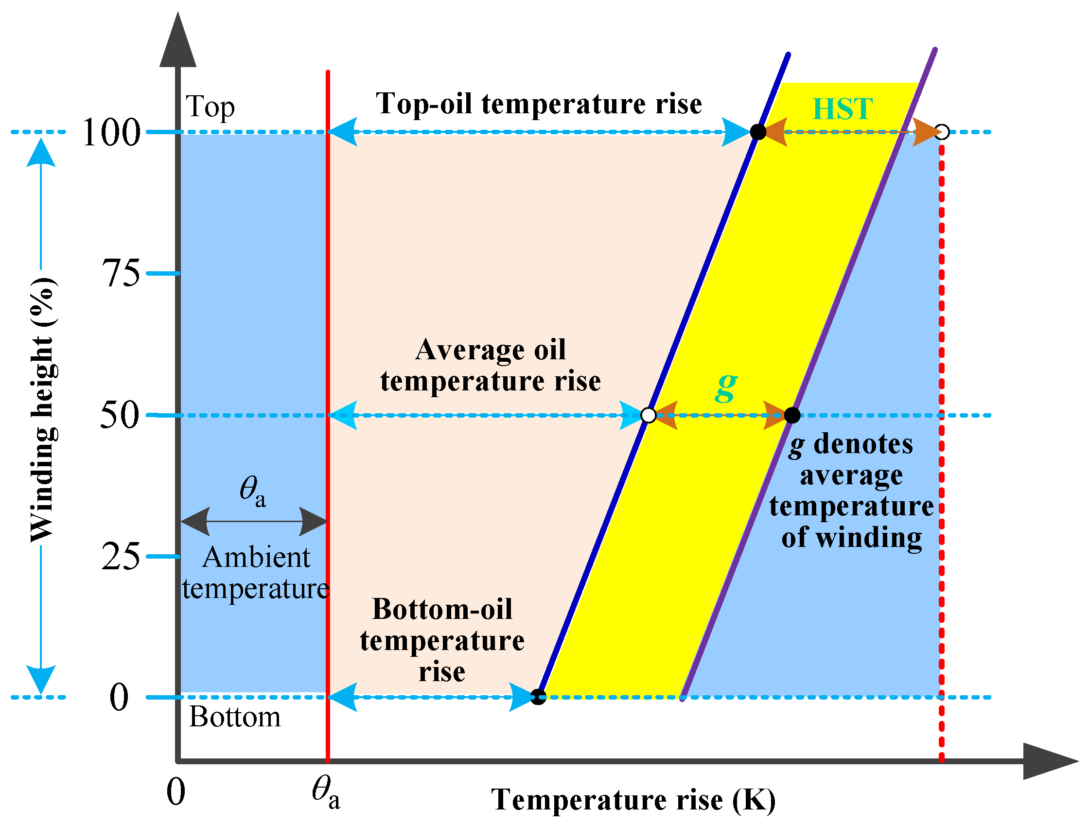
2.1. Internal Temperature Characteristics of the Large Oil-Immersed Transformer

There are many factors that can affect the oil-paper insulation property of the transformer, which cause insulation ageing. Among them, the factors that influence the transformer internal temperature, especially the winding HST [2], are the core ones to the TOPIS [35]. At present, the exact position of transformer hot spot is very difficult to be determined while most transformers haven’t been installed with temperature sensors; in particular, future installation of such sensors is relatively difficult to be realized. To address this issue, so far, thermal characteristic based model has been widely adopted to study the thermal operation of transformer. In addition, IEEE Std. C57.91-2011 [36] and IEC 60076-7—Power Transformers—Part 7 [37] recommended an empirical model to calculate transformer winding HST. Here, the former one defined the empirical equations to calculate the top-oil temperature and winding HST of the transformer while the latter one assumed that the temperature rise curves of the winding distribution and oil distribution are two parallel straight lines, as shown in Figure 1. It can be found that the winding HST is obtained by the ambient temperature, top-oil and bottom-oil temperatures, and temperature gradient of winding hot spots with respect to the oil temperature. Note that the HST calculation method in IEEE standard [36] was employed in this paper to solve the winding HST.

2.2. Weibull Distribution Based Failure Rate Function

The Weibull distribution model, as a kind of monotonous failure rate distribution model, is adopted in this paper to investigate the failure rate of TOPIS after the winding HST is obtained due to the merit of a closer representation of stochastic events, such as the lifetime and reliability of the product, as well as multiple deformation modes of failure rate [38], and it is defined by:

$$\lambda (t)=\frac{\beta t^{\beta -1}}{{\eta }^{\beta }}$$

(1)

where λ(t) is the Weibull distribution based failure rate function. η is the scale parameter, β is the shape parameter, and t is the time in year, with η > 0, β > 0 and t ≥ 0. The corresponding probability density function is given by $f(t)=(\beta t^{\beta -1}/{\eta }^{\beta })\exp [-{(t/\eta )}^{\beta }]$, the degree of reliability is described as $R(t)=\exp [-{(t/\eta )}^{\beta }]$, and the failure distribution function is written as $F(t)=1-\exp [-{(t/\eta )}^{\beta }]$, respectively.

Equation (1) is adequate to illustrate various equipment failure rates by carefully varying the system parameters, namely β and η, thus it has a strong compatibility. Here, several examples are given as follows:

• $\beta =1$, representing an exponential distribution.
• $\beta =2$, representing a Rayleigh distribution.
• $\eta =1$, $\beta >1$, representing a monotonic increasing function that can illustrate the failure rate of equipment in a wearing stage.
• $\eta =1$, $\beta =1$, representing the failure rate of equipment in a long-term failure stage.
• $\eta =1$, $0<\beta <1$, representing a monotonic increasing function that can describe the early failure rate of equipment.

Hence, this Weibull distribution model can describe the failure of the ageing equipment during the failure stage very well. The parameters β and η can be obtained based on the maximum likelihood estimation method (MLEM) [32] as follows:

$$\ln L(\theta /\mathit{X})=\ln L(x_1,x_2,\cdots ,x_n;\theta )={\displaystyle \sum _{i\in \mathit{F}}(\ln \beta +(\beta -1)\ln x_i-\beta \ln \eta }-{(x_i/\eta )}^{\beta })+\sum _{i\in \mathit{C}}(-{(x_i/\eta )}^{\beta })$$

(2)

where F is the failure data set. C is the truncated data set. X = (x₁, x₂,…, x_n) is the data sequence, which has failure data and truncated data. θ is a model parameter to be evaluated.

Based on (2), β and η can be solved by:

$$\{\begin{array}{l}\frac{\partial \ln L(\theta /\mathit{X})}{\partial \beta }={\displaystyle \sum _{i\in \mathit{F}}(1/\beta +\ln x_i-\ln \eta -{(x_i/\eta )}^{\beta }\ln (x_i/\eta ))}+{\displaystyle \sum _{i\in \mathit{C}}(-{(x_i/\eta )}^{\beta }\ln (x_i/\eta ))=0}\\ \frac{\partial \ln L(\theta /\mathit{X})}{\partial \eta }={\displaystyle \sum _{i\in \mathit{F}}(-\beta /\eta +(\beta /\eta ){(x_i/\eta )}^{\beta })}+{\displaystyle \sum _{i\in \mathit{C}}((\beta /\eta ){(x_i/\eta )}^{\beta })=0}\end{array}$$

(3)

In practice, the MLEM chooses proper parameters of the Weibull distribution model to generate a maximum probability of occurrence of the samples, which values are used as point estimations of unknown parameters.

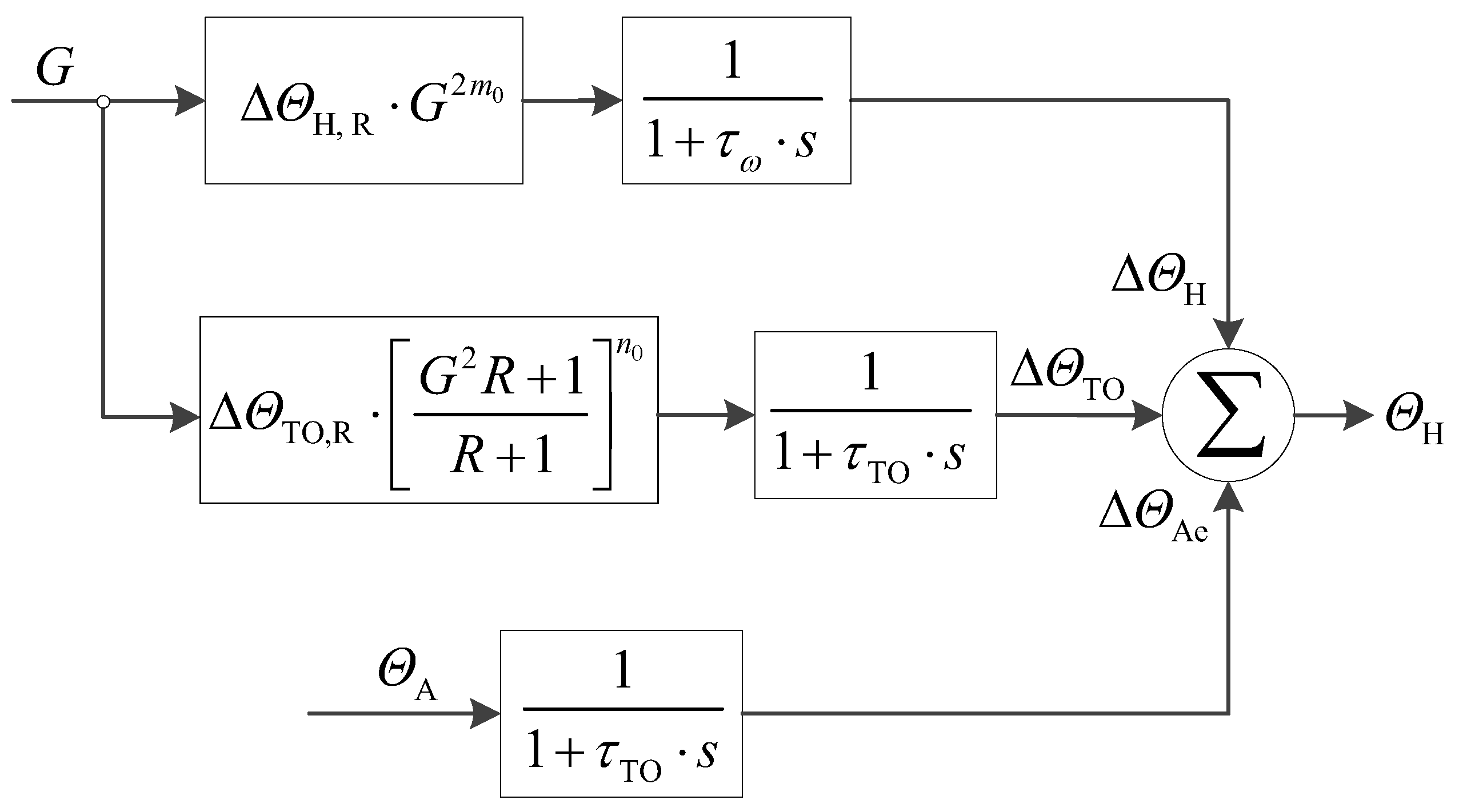
2.3. Transformer Winding HST Calculation

The failure rate of transformer in ageing of insulation is closely related to the winding HST, this is mainly determined by the ambient temperature and the load of the transformer. The hottest point is usually located on the top/middle part of the low-/high-voltage winding of the transformer. Based on the calculation method of winding HST recommended in [36], the calculation flowchart of this method is depicted in Figure 2, where R is the ratio of load loss to no-load loss at a rated load. s is the complex frequency. τ_ω is the time constant in temperature point position in hour. τ_TO is the time constant of transformer oil in hour. ΔΘ_TO,R is the top-oil temperature rise at the rated load, °C. ΔΘ_H,R is the temperature rise of winding HST with respect to the top-oil temperature at the rated load, °C. ΔΘ_H is the increment of winding HST with respect to the top-oil temperature, °C. ΔΘ_TO is the top-oil temperature rise with respect to the ambient temperature, °C. ΔΘ_Ae is the delayed ambient temperature, °C; ΔΘ_A is the instantaneous ambient temperature, °C; m₀ and n₀ are empirical constants determined by the cooling modes: for the cooling modes of Oil Natural Air Natural (ONAN), Fan Air (FA), Force Oil-circulated (via pump) Air (FOA) and Force Oil-circulated Water (FOW), m₀ and n₀ are chosen to be 0.8 and 0.9, respectively, while for the modes of indirect FOA and indirect FOW, m₀ and n₀ are both taken to be 1.0. G is the ratio of the actual load of the transformer to the rated load, and note that the calculation of the G below is related to the specific load changes. The value of G can be determined by the following formula compared with the equivalent load of the full-day fluctuating loads [39], and here the equivalent value is G when the per-unit value is taken, namely:

$$G=\sqrt{{\displaystyle \sum _{k=1}^{k=N_{\mathrm{c}}}{L}_k^2{t}_k}/{\displaystyle \sum _{k=1}^{k=N_{\mathrm{c}}}{t}_k}}$$

(4)

where L_k is the equivalent constant load of each time period. N_c is the number of equivalent time periods within a cycle period. t_k is the length of the set time period.

In general, four steps are needed to realize the above procedure and they are briefly demonstrated as follows:

Step 1: Calculate the top-oil temperature rise ΔΘ_TO according to the ambient temperature as:

$$\{\begin{array}{l}{\tau }_{\mathrm{TO}}\frac{\mathrm{d}\Delta {\Theta }_{\mathrm{TO}}}{\mathrm{d}t}=\Delta {\Theta }_{\mathrm{TO},\mathrm{U}}-\Delta {\Theta }_{\mathrm{TO}}\\ \Delta {\Theta }_{\mathrm{TO},\mathrm{U}}=\Delta {\Theta }_{\mathrm{TO},\mathrm{R}}\cdot {(\frac{G^{2}R+1}{R+1})}^{n_0}\end{array}$$

(5)

where ΔΘ_TO,U is the final rise of the top-oil temperature with respect to the ambient temperature, °C. Moreover, one can yield ΔΘ_TO = ΔΘ_TO,U if the dynamics of temperature variation is ignored (i.e., $\frac{\mathrm{d}\Delta {\Theta }_{\mathrm{TO}}}{\mathrm{d}t}$ is close to zero). Lastly, ΔΘ_TO,R can be obtained by actual tests [40].

Step 2: Calculate the increment of winding HST, namely ΔΘ_H, based on the transformer top-oil temperature by:

$$\{\begin{array}{l}{\tau }_{\omega }=\frac{\mathrm{d}\Delta {\Theta }_{\mathrm{H}}}{\mathrm{d}t}=\Delta {\Theta }_{\mathrm{H},\mathrm{U}}-\Delta {\Theta }_{\mathrm{H}}\\ \Delta {\Theta }_{\mathrm{H},\mathrm{U}}=\Delta {\Theta }_{\mathrm{H},\mathrm{R}}\cdot G^{2m_0}\end{array}$$

(6)

where ΔΘ_H,U is the final increment of the highest temperature point based on the top-oil temperature, °C; and ΔΘ_H,R is the temperature rise of the hottest point with respect to the oil temperature at the rated load, °C; Again, one can obtain ΔΘ_H = ΔΘ_H,U if the dynamics of temperature variation is ignored (i.e., $\frac{\mathrm{d}\Delta {\Theta }_{\mathrm{H}}}{\mathrm{d}t}$ is close to zero).

Step 3: Calculate the delayed ambiance temperature ΔΘ_Ae (°C) by:

$${\tau }_{\mathrm{TO}}\frac{\mathrm{d}\Delta {\Theta }_{\mathrm{Ae}}}{\mathrm{d}t}={\Theta }_{\mathrm{A}}-{\Theta }_{\mathrm{Ae}}$$

(7)

Similarly, it arrives ΔΘ_A = ΔΘ_Ae if the dynamics of temperature variation is neglected (i.e., $\frac{\mathrm{d}\Delta {\Theta }_{\mathrm{Ae}}}{\mathrm{d}t}$ is close to zero).

Step 4: Based on Step 1 to Step 3, the winding HST, namely ΔΘ_H (°C) is finally obtained by:

$${\Theta }_{\mathrm{H}}=\Delta {\Theta }_{\mathrm{TO}}+\Delta {\Theta }_{\mathrm{H}}+\Theta {\Delta }_{\mathrm{Ae}}$$

(8)

2.4. Transformer Failure Rate λ Calculation

The ageing of winding insulation system for the oil-immersed power transformer is unidirectional and irreversible. In fact, the mechanical property, dielectric strength and resistance will be gradually degenerated along with the time, which might result in a transformer failure or even an end of transformer life. Hence, after obtaining the winding HST namely Θ_H (°C) via calculation, the expected life of the winding insulation system can be obtained. Here, the relationship between temperature and chemical reaction rate of insulation materials can be written as:

$$L=C\exp (\frac{B}{T+273})$$

(9)

where L is the expected life of insulation material, here it represents the expected life of the winding insulation system; coefficients B and C are related to the insulation material type and activation energy from the resistance-to-high temperature tests; and T is the thermal temperature of winding, here it refers to the winding HST, which has been obtained in Section 2.3.

If the Weibull distribution model is adopted to describe the ageing process of the winding insulation system, together with the assumption of η = L, the failure rate function in (1) can be written as λ(t) = βt^β−1/L^β. Furthermore, when the obtained winding HST is substituted into (9), i.e., make T = Θ_H, the L can be obtained. Finally, substitute T and L into (1), then the failure rate function λ(t) under Θ_H can be rewritten as:

$$\lambda (t)=\beta t^{\beta -1}{\left[C\exp (\frac{B}{{\Theta }_{\mathrm{H}}+273})\right]}^{-\beta }$$

(10)

where the parameters β, B, and C are obtained by MLEM. Based on [41] and the Gaussian distribution, a new approach is proposed to estimate these parameters, including the following two steps: (i) Estimate the parameters of η and β in Weibull distribution model according to the standard deviation σ and the desired value μ in Gaussian distribution; and (ii) Maintain β, adopt η to estimate B and C in (10).

3. Dynamic Correction Model

The above static model or the base model can only be used to simulate the failure rate of TOPIS when a transformer is in the ideal ageing process. However, some unpredictable factors, e.g., the partial discharge, high-temperature, and overheat, may occur in the actual operation of the transformer. As a result, an accurate system modelling is required to take these uncertainties into account, such that a more satisfactory prediction can be ensured.

3.1. Grey Target Theory

The grey-system theory [42,43] is a theoretical result developed on the basis of the practice of fuzzy mathematics, which mainly extracts valuable information from the generation and development of partial known information of the research object, so as to achieve the correct understanding and effective control of the research system behavior. Here, the grey-correlation analysis of the transformer failures means the identification and classification of the symptom modes and fault modes. In general, the steps of the analysis are as follows: Firstly, construct a comparative sequence based on the input DGA data; secondly, use the grey-correlation analysis to calculate the grey-correlation degree between the comparative sequence and the reference sequence; thirdly, compared with the grey correlation degree, the principle to be followed is that the greater the grey-correlation degree is, the closer the actual fault mode and the reference fault mode are.

In this paper, the grey target theory in the grey-system theory has been used, which contains the grey-assessment and grey decision-making theory. The gist of grey target theory is at first to set a grey target under the condition of no standard modes, in which find the bull’s-eye via the grey-system theory; and then, compare the model of each index with the standard model; and finally, determine the assessment grade via the grad division. Concretely, the grey target theory used in this paper is briefly introduced as follows:

(1) Determine the standard evaluation mode: Assume that ${\omega }_i$ is the ith state mode of the equipment, and $\omega (k)$ is the kth state parameter sequence for the equipment state monitoring, and then the standard state mode ${\omega }_0$ is set up as follows. First, make ${\omega }_i=\{{\omega }_i(k)|k=1,2,\cdots n\}$, then for $\forall {\omega }_i(k)\in {\omega }_i$, it obtains $k\in K=\{1,2,\cdots n\}$ and $i\in I=\{1,2,\cdots m\}$; second, make $\omega (k)=\{{\omega }_i(k)|i=1,2,\cdots m\}$, then for $\forall {\omega }_i(k)\in \omega (k)$, it obtains $i\in I=\{1,2,\cdots m\}$, where $\omega (k)$ is called index mode sequence, and m is the sum total of the index modes . In general, the polarity of the index has three categories as maximum polarity, minimum polarity, and medium polarity, which are represented as POL_max, POL_min and POL_med, and then the selection of standard evaluation model elements is based on as:

$$\mathrm{make}{\omega }_0(k)=\{\begin{array}{c}\underset{i}{\max }{\omega }_i(k),{\omega }_i(k)\in \omega (k)\mathrm{if}POL\omega (k)=PO{L}_{\max }\\ W_0\mathrm{or}\underset{i}{\mathrm{avg}}{\omega }_i(k),{\omega }_i(k)\in \omega (k)\mathrm{if}POL\omega (k)=PO{L}_{\mathrm{med}}\\ \underset{i}{\min }{\omega }_i(k),{\omega }_i(k)\in \omega (k)\mathrm{if}POL\omega (k)=PO{L}_{\min }\end{array}$$

(11)

where W₀ is an assigned value. $\underset{i}{\mathrm{avg}}{\omega }_i(k)$ means take the average of ${\omega }_i(k)$, $i=1,2,\cdots m$. The sequence $\{{\omega }_i(1),{\omega }_i(2),\cdots ,{\omega }_i(n)\}$ is called object standard evaluation model. ${\omega }_0=\{{\omega }_0(1),{\omega }_0(2),\dots ,{\omega }_0(n)\}$ is the standard state mode or bull’s-eye. The approaching degree is related to the index, and the grey target contribution index is to study the effect of the index on the size of the mode approaching degree.

(2) Grey target transformation: Assume that the state mode of the object to be made grey target transformation is the object evaluation model at the moment j, namely $\{{\omega }_j^{\prime }(1),{\omega }_j^{\prime }(2),\cdots ,{\omega }_j^{\prime }(n)\}$, here, GTT means the grey target transformation, then ${\omega }_j^{\prime }$ and ${\omega }_0$ are made grey target transformation as:

$$GTT{\omega }_j^{\prime }(k)=\min ({\omega }_j^{\prime }(k),{\omega }_0(k))/\max ({\omega }_j^{\prime }(k),{\omega }_0(k))=x_j(k)$$

(12)

where $k=1,2,\cdots ,n$, and $j\in J=\{1,2,\cdots ,N\}$. Here, N means the sum total of the state modes to be evaluated, generally N is took 1. Under this transformation, the grey target transformation value under the standard evaluation mode can be obtained as $\mathrm{TTG}{\omega }_0=x_0=\{x_0(1),x_0(2),\cdots ,x_0(n)\}=\{1,1,\cdots ,1\}$, called the standard bull’s-eye (or the standard target).

(3) Calculate the grey-correlation coefficient: The grey-correlation coefficient in the grey-correlation difference information space corresponding to the contribution factor set is described as:

$$\gamma (x_0(k),x_j(k))=\frac{\underset{j}{\min }\underset{k}{\min }{\Delta }_j(0,k)+\xi \underset{j}{\max }\underset{k}{\max }{\Delta }_j(0,k)}{{\Delta }_j(0,k)+\xi \underset{j}{\max }\underset{k}{\max }{\Delta }_j(0,k)}$$

(13)

where $\xi$ is the contribution coefficient of the kth index under the mode j (i.e., at the moment j), and $\xi \in [0,1]$. ${\Delta }_j(0,k)=|x_0(k)-x_j(k)|=|1-x_j(k)|$.

(4) Calculate the approaching degree: The approaching degree (i.e., the grey-correlation degree) can be calculated as:

$$\gamma (x_0,x_j)=\frac{1}{n}{\displaystyle \sum _{k=1}^n\gamma (x_0(k),x_j(k))}$$

(14)

where $\gamma (x_0,x_j)$ represents the degree of the bull’s-eye of a mode close to that of the standard state mode, called the approaching degree.

(5) Calculate the weighted approaching degree: Take ${\gamma }_{\mathrm{mea}}$ as the average value of the contribution degree of all the indexes, thus the weight that corresponds to ${\gamma }_{\mathrm{mea}}$ should be 1/n. Then the weight value is determined by the proportion of the difference in the average value, here the difference means the difference between the contribution degree of each index and the average value of the contribution degree (i.e., ${\gamma }_{\mathrm{mea}}$). Hence, the formula is constructed as:

$$q_i=\{\begin{array}{c}\frac{1}{n}(1+\frac{|{\gamma }_{\mathrm{mea}}-\gamma (i)|}{{\gamma }_{\mathrm{mea}}}),\mathrm{if}\gamma (i)>{\gamma }_{\mathrm{mea}}\\ \frac{1}{n}(1-\frac{|{\gamma }_{\mathrm{mea}}-\gamma (i)|}{{\gamma }_{\mathrm{mea}}}),\mathrm{if}\gamma (i)<{\gamma }_{\mathrm{mea}}\end{array}\mathrm{here},{\displaystyle \sum _{i=1}^n{q}_i}=1$$

(15)

where i is the number of the index. n is the sum total of the indexes. q_i is the weight value.

Then, the approaching coefficient is:

$$\gamma ({\omega }_0(k),{\omega }_i(k))=\frac{\underset{i}{\min }\underset{k}{\min }{\Delta }_{0i}(k)+\rho \underset{i}{\max }\underset{k}{\max }{\Delta }_{0i}(k)}{{\Delta }_{0i}(k)+\rho \underset{i}{\max }\underset{k}{\max }{\Delta }_{0i}(k)}$$

(16)

where $\rho \in [0,1]$. ${\Delta }_{0i}(k)$ represents the grey-correlation difference information between the sequence to be evaluated ${\omega }_i$ and the bull’s-eye ${\omega }_0$.

Finally, the approaching degree of ${\omega }_i$, namely $\gamma ({\omega }_0,{\omega }_i)$ can be obtained as:

$$\gamma ({\omega }_0,{\omega }_i)={\displaystyle \sum _{k=1}^n\gamma ({\omega }_0(k),{\omega }_i(k))q_k}$$

(17)

which means the degree of each mode close to the standard state mode.

(6) Determine the grade of evaluation object: The grade of the evaluation object is determined by the approaching coefficient. Based on the principle of equilibrium in the grey-system theory, each target can be set at a level of 0.1 between 0 and 1, namely [0.9, 1], [0.8, 0.9], …, [0.0, 0.1]. In addition, according to the relevant theorems of grey-correlation degree, under the situation of $\underset{i}{\max }\underset{k}{\max }{\Delta }_{0i}(k)=0$ and $\xi =\rho =0.5$, we obtain:

$$0.33333=\frac{\xi }{1+\xi }\le \gamma ({\omega }_0(k),{\omega }_i(k))\le 1,\forall k\in K=\{1,2,\dots ,n\}$$

(18)

which means that $\gamma ({\omega }_0,{\omega }_i)\ge 0.33333$. Hence, the grades below [0.3, 0.4] are meaningless. The grade that the approaching degree is in refers to the grey evaluation grade.

In addition, different weight values can be assigned to different performance indexes when the importance of them to the evaluation results is different, thus the greater the weight is, the more important the corresponding performance index to the evaluation results, which may be more consistent with the actual situation, and can also better distinguish their contribution to the results of the evaluation. Hence, make λ_k represent the weight value of each performance index, here k = 1, 2, …, n. The value of λ_k can be obtained via the analytic hierarchy process (AHP), thus the grey target theory based approaching degree in this approach can be calculated as:

$$\gamma (x_0,x_j){|}_{\lambda ={\lambda }_k}={\lambda }_k\cdot \gamma (x_0(k),x_j(k)),k=1,2,\cdots ,n,j=1,2,\cdots ,N$$

(19)

Here, the AHP is a multi-object decision-making analysis method combing qualitative and quantitative analysis methods, in which the elements that are always related to decision-making are decomposed into goals, guidelines, schemes and other levels. It generally contains three steps as follows: construct an expert judgment matrix, calculate the weight value of the judgment matrix, and the consistency test. The specific description of these steps can be referred to [43,44].

3.2. Characteristic Gases Selection

Under normal circumstances, no characteristic gases are produced when the transformer is under operation. However, if a local overheating or a high-temperature electric arc emerges in the transformer, these characteristic gases will be rapidly generated and gradually dissolved into the transformer oil. This indicates an internal failure would occur in the transformer and may significantly shorten the life expectancy of TOPIS, which has an exponential relationship with its winding HST [45]. Therefore, the equivalent HST can be obtained via the corrections of transformer life expectancy, such that the impacts of the transformer failures, such as the local overheating and electric arc overheat on the transformer insulation can be quantified via the equivalent HST.

Here, the hydrogen (H₂), methane (CH₄), ethane (C₂H₆), ethylene (C₂H₄) and acetylene (C₂H₂) in DGA are selected as condition assessment indices of the oil-paper insulation of the transformer. The relationship between these gases and internal failures are demonstrated in

Table 1. Gases generated by different failure types.

Failures	Main Gas Components	Petit Gas Components
Oil overheating	CH4, C2H4	H2, C2H6
Oil and oil paper overheating	CH4, C2H4, CO, CO2	H2, C2H6
Partial discharge in TOPIS	H2, C2H2	C2H2, C2H6, CO2
Spark discharge in oil	H2, C2H2	/
Electric arc in oil	H2, C2H2	CH4, C2H4, C2H6
Electric arc in oil and oil-paper	H2, C2H2, CO, CO2	CH4, C2H4, C2H6

. Note that these gases are chosen as characteristic gases because the power supply enterprises do not have the condition of testing the DP at the present stage, and besides, the tests on the content of furfural (a kind of a chemical) are rarely conducted, such that it is very difficult to obtain the characteristic parameters. Moreover, the operation of transformer oil filtration and maintenance has a great influence on the content of furfural, which affects the accuracy of the model and thus causes the model to be difficult to popularize. In contrast, DGA data is large and easy to obtain, i.e., it can be obtained via both off-line mode and on-line monitoring mode, such that the DGA data for condition assessment has unique advantages.

The transformer health grade is closely related to transformer life expectancy, i.e., when the transformer runs well, and then the life expectancy of the TOPIS will be extended; meanwhile when the transformer is in bad health, and then the deterioration of the TOPIS will be accelerated and the life expectancy will be shortened. Hence, in order to develop such relationship between transformer health grade and transformer life expectancy, a life correction model of the transformer needs to be proposed after consulting the model framework of deterioration degree.

3.3. Grey Target Theory-Based Dynamic Correction

Hence, based on the above grey target theory, the data processing attempts to obtain the grey approaching degree Q_i, with 0.33 ≤ Q_i ≤ 1.0 and i = 1, 2, 3, 4, 5 to evaluate the grade of health state by the following five intervals: [0.9, 1.0], [0.6, 0.9), [0.5, 0.6), [0.4, 0.5), and [0.33, 0.4), respectively. In addition, the gradation coefficients α_i and δ_i (here, i = 1, 2, 3, 4) are introduced to properly adjust the corresponding relationships between the failure degree of TOPIS and transformer life expectancy. Here, α_i are used to regulate the proportional relationship between the approaching degree and transformer life expectancy while δ_i are introduced to consider the case when the linear relationship between the approaching degree and transformer life expectancy may not be satisfied. Moreover, the larger δ_i are, the smoother the corresponding life shortening will be. Lastly, their values are determined by the expert evaluations and detailed as follows:

• If i = 1, 2, 3, and 4, the health states of the TOPIS are graded into four levels, respectively, e.g., health, normal, slight failure, and medium failure. The correction coefficients L_i of transformer life expectancy of the four health grades are defined as:

  $$L_i={\alpha }_i{(\frac{Q_i-0.33}{1-0.33})}^{{\delta }_i}i=1,2,3,4$$

  (20)

  where the grey approaching degree Q_i can be chosen by:

  $$Q_i\in \{\begin{array}{c}[0.9,1.0],\mathrm{if}i=1\\ [0.6,0.9),\mathrm{if}i=2\\ [0.5,0.6),\mathrm{if}i=3\\ [0.4,0.5),\mathrm{if}i=4\end{array}$$

  (21)
• If i = 5, it means a serious failure (the lowest rank). Under such condition, if the transformer is maintained well, the homologous failure rate of TOPIS can be calculated according to the recovery after maintenance, as well as the life loss recovery factor.
  Finally, the life expectancy Z_eq after correction is described as:

  $$Z_{\mathrm{eq}}={\alpha }_i{(\frac{Q-0.33}{1-0.33})}^{{\delta }_i}Z,i=1,2,3,4,Q\in [0.4,1.0]$$

  (22)

  where Z is the original life expectancy solved by the static model (i.e., the base model). The life loss ∆Z′ after correction is defined as:

  $$\Delta Z^{\prime }=[1-{\alpha }_i{(\frac{Q-0.33}{1-0.33})}^{{\delta }_i}]Z$$

  (23)

  where α_i and δ_i (i = 1, 2, 3, 4) are empirical variables and should be determined according to the historical operation data and maintenance data of actual transformer. For illustration purposes, it is assumed that there is a strict proportional relationship between the life loss variable ∆Z′ of TOPIS and the state variable of transformer. Let α_i = δ_i = 1 (i = 1, 2, 3, 4), then the corresponding relationship between the approaching degree, value range of life expectancy correction coefficients, and transformer health state grade is shown in

  Table 2. Corresponding relationship between the state grade and life expectancy correction coefficient of transformer oil-paper insulation system (TOPIS).

  Range of Approaching Degree Q	State Grade	Life Expectancy Correction Coefficient L
  [[0.9,1.0]	Health state	[[0.85,1.00]
  [0.6,0.9)	Normal state	[0.40,0.85)
  [0.5,0.6)	Slight failure	[0.25,0.40)
  [0.4,0.5)	Medium failure	[0.10,0.25)
  [0.33,0.4)	Serious failure	[0,0.10)

  .

In Table 2, it can be seen that the winding HST is the core factor or the connection link between the static evaluation model (i.e., the base model) and the dynamic correction model. Here, the corresponding relationship between the state value and winding HST can be obtained via the transformer state data processing with the grey target theory based correction model, such that the equivalent winding HST can be calculated and the dynamic corrections of the base model can be made. The flow chart of dynamic correction modelling based on the grey target theory is shown in Figure 3.

3.4. Second Model Correction after Maintenance

When the transformer is in operation, the maintenance of TOPIS is carried out based on its operational condition, which is an interruption for status continuity of the transformer. After that, the life expectancy of the transformer can be extended, with a reduction of the equivalent HST.

With regard to the concept of age reduction factor in [45], the life expectancy loss recovery factor χ is introduced in this paper. The life expectancy Z″ of the transformer after maintenance that involves its winding oil-paper insulation system, such as a major maintenance or an oil separation, is calculated as:

$$Z^{″}=Z_{\mathrm{eq}}+\chi Z_{\mathrm{eq}}^{\prime }$$

(24)

where Z″, Z_eq and Z′_eq are the new life expectancy of the transformer, corrected life expectancy before the last maintenance and corrected life loss before the last maintenance, respectively. The original model can be modified by using the equivalent HST (H_eq), which is related to the life expectancy. The final failure rate λ_a(t) after the dynamic corrections is obtained as:

$${\lambda }_{\mathrm{a}}(t)=\beta t^{\beta -1}{(C{\mathrm{e}}^{\frac{B}{H_{\mathrm{eq}}+273}})}^{-\beta }$$

(25)

Note that, this failure rate is geometrically corrected from a static exponential curve to a dynamic stair-stepping one.

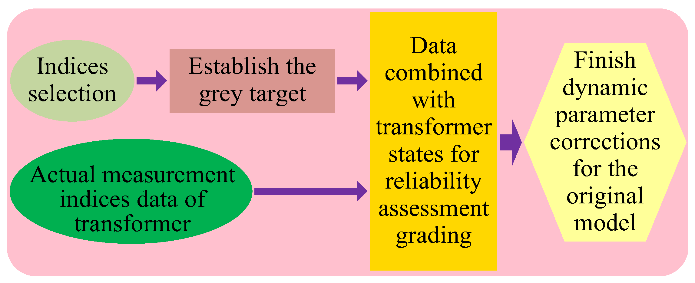
3.5. Framework Establishment of the Final Model

According to the HST based static ageing failure model and grey target theory based dynamic correction model combing with the DGA method, the final framework of the whole reliability assessment model of the TOPIS is illustrated in Figure 4.

4. A Case Study

As discussed previously, DGA contains a large amount of data, which can be easily obtained by offline or online monitoring approach, thus it becomes an effective characteristic quantity to study the internal characteristics of the transformer. Based on DGA, the TOPIS is selected as the evaluation objective, and in this section, a practical case study is carried out with the ultimate transformer reliability assessment model developed in previous section. In this case study, the dynamic corrections are performed based on the actual DGA data from the Jiangmen Power Supply Bureau in China Southern Power Grid. Here, a conclusive failure rate curve with dynamic corrections is obtained, which can effectively track the actual operation status of the transformer, and accurately reflect its actual reliability level and the ageing process. The case study is discussed as follows.

4.1. Parameters Selection

The main transformer (numbered #2) is considered in the practical case study, which is from a 110 kV substation located in the Jiangmen Power Supply Bureau of Guangdong Power Grid Corporation of China (Jiangmen, China), and it has been operating since 2002. The designed parameters of this transformer are determined as follows: The transformer type is SFZ8-40000/110 (PuBo Technological Electricity Co., Ltd, Shanghai, China), rated voltage is 110 kV, rated capacity is 40 MVA, winding/top-oil temperature rise is 65 K/55 K, no-load loss is 33.8 kW, load loss is 178.1 kW, cooling mode is ONAN, ΔΘ_TO,R is 36.0 °C and ΔΘ_H,R is 28.6 °C. The parameters of TOPIS reliability evaluation model are given as B = 1500, C = 0.56, τ_TO,R = 3.5 h, χ_i = 0.5, χ_j = 0.8, m₀ = 0.8, n₀ = 0.8, and R = 5.3. Here, the empirical factors χ_i and χ_j are the life expectancy lost recovery factors of the transformer in oil separation and major maintenance, respectively. At last, τ_TO,R is the time constant of transformer oil obtained at rated load in hour.

The temperature curve of Jiangmen is given by the Jiangmen Meteorological Bureau in southern China, and the statistic interval is selected from the years of 1957 to 2013, while the average yearly temperatures of each January are demonstrated in Figure 5.

The average yearly temperature is selected as the temperature reference, which is the average value of 57 groups of temperature data from 1957 to 2013. Based on these monthly average temperatures, the average temperatures of 12 months (i.e., from January to December) are 13.9, 15.4, 18.1, 23.2, 25.8, 27.6, 28.6, 29.2, 28.3, 25.5, 21.4 and 17.9 °C, respectively.

4.2. Transformer Load Rate Curve

In order to calculate the winding HST and reflect the actual load-bearing ability of the power transformer, as well as obtain the load rate curve, the following aspects are considered as follows.

• In the short term, the load of a transformer is varied with a daily characteristic, called a daily cycle curve;
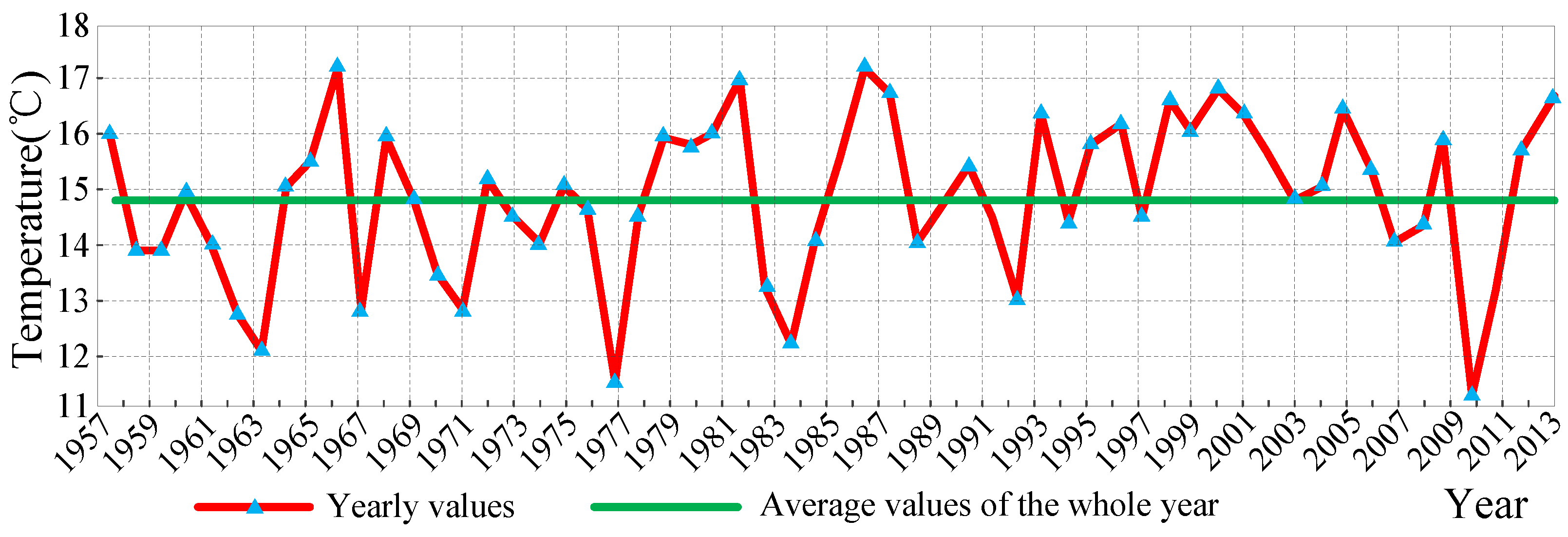
• In the long term, the load of a transformer is changed with a yearly characteristic, called a yearly cycle curve, while there are also some seasonal regulations in loads. In order to completely describe the load fluctuation, the calculation and feasibility should be considered.

Based on above considerations, two equivalent schemes are carried out as

• Select the load levels on the first, eleventh and twenty-first days of each month, which equal to 36 days in a whole year.
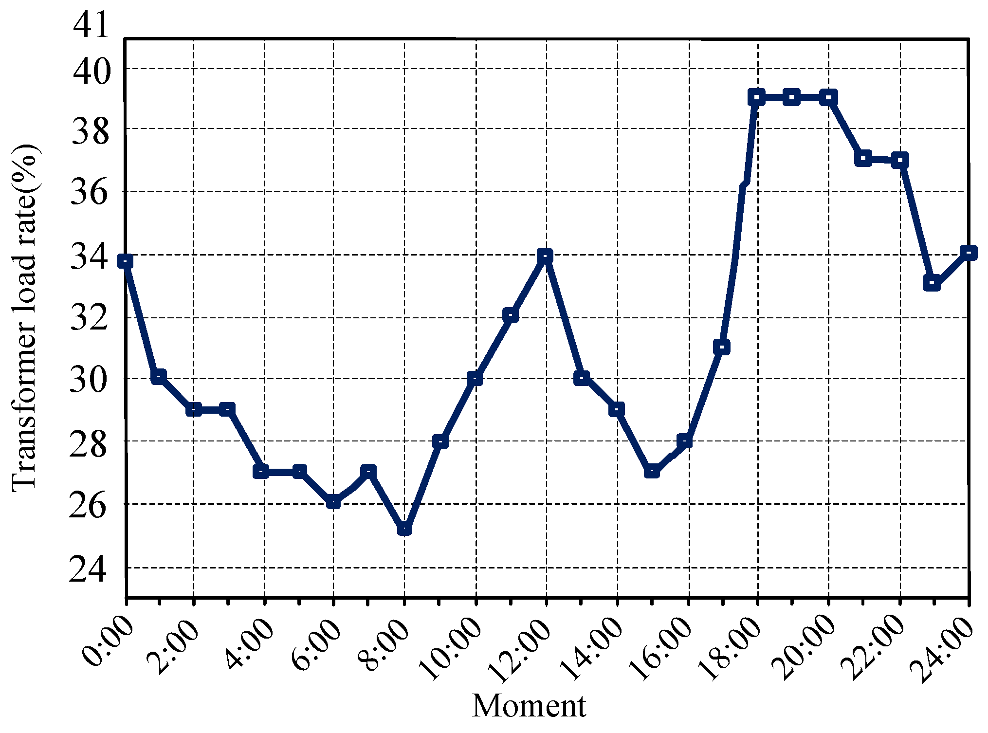
• Discretize the load curve in each hour. In practice, the transformer load is usually measured in terms of current. The per unit load rate is chosen as the ratio of the actual current to the nominal current. For example, the load rate curve of the main transformer on 1 January, 2013 is shown in Figure 6.

4.3. Winding HST Calculation

After discretization of the winding HST rise in each hour, as shown in Figure 7, the average HST for a whole day is calculated as:

$${\Theta }_{\mathrm{HD}}={\displaystyle \sum _{i=1}^{24}{\Theta }_{\mathrm{H}i}/24=30.24}{(}^{\circ }\mathrm{C})$$

(26)

Without loss of generality, the average winding HST of other sampling days can be similarly calculated. Thus, the average of temperatures in these 36 groups of sampling days can be regarded as the yearly average HST, namely:

$${\Theta }_{\mathrm{HY}}={\displaystyle \sum _{j=1}^{36}{\Theta }_j/36=43.42}{(}^{\circ }\mathrm{C})$$

(27)

4.4. Failure Rate Calculation

In work [45], the life distributions of 154 transformers were analyzed statistically. The empirical values of the Arrhenius equation using Gaussian distribution can be determined. The simulation is performed in Matlab and the relationship between winding HST and life expectancy is presented in Figure 8, from which the life expectancy can reach 64.12 (year) when the winding HST is 43.42 °C. Substitute the obtained temperature and related parameters into (1), the failure rate can be calculated as:

$${\lambda }_{\mathrm{a}}(t|43.42)=5\times {[0.56\exp (\frac{1500}{43.42+273})]}^{-5}{t}^4\approx 4.6141\times {10}^{-9}{t}^4$$

(28)

The relationship between the failure rate of TOPIS λ (%) and the transformer characteristic life t (year) is indicated in Figure 9. It can be observed that the failure rate of TOPIS, which has been in operation for 12 years, is only 0.01%. The reason for such a low failure rate can be explained as the operating condition has been quite good, with a load rate around 40%. However, there may be some practical cases that should be considered in the operation of a transformer, such as short-time overload, inrush current, etc. In addition, improper design can also be considered as a core factor dramatically influencing the failure rate of TOPIS. Therefore, it needs to correct the failure rate with considerations of the above aspects.

4.5. Dynamic Corrections Based on DGA Data

The failure rate curve of TOPIS can be dynamically corrected based on actual DGA data. The DGA testing data of the main transformer (#2) in substation are shown in

Table 3. Dissolved gas analysis (DGA) testing data from year of 2002 to 2014.

Date (Year)	Gas Contents (μL/L)
	H2	CH4	C2H6	C2H4	C2H2
2002	3	1.2	1	0	0
2003	6	3.2	0	2.1	0
2004	7	5.49	0.85	3.03	0
2005	4	6.22	0.99	3.1	0
2006	4	8.53	1.24	3.49	0
2007	4	10.25	1.63	4.16	0
2008	3	11.7	1.8	4.14	0
2009	3	11.66	1.79	4.14	0
2010	2	14.86	2.09	3.81	0
2011	3	13.02	1.84	3.14	0
2012	3	13.8	2.06	3.2	0
2013	0	19.72	3.06	3.65	0
2014	0	18.82	3.08	3.53	0

, which are obtained from the Maintenance Department of Jiangmen Power Supply Bureau.

It can be seen from Table 3 that the DGA data are continuous and no maintenances are carried out on the winding insulation system in the transformer, e.g., the disintegration maintenances, and the oil separations. As there is an accumulation in the DGA data, it’s necessary to correct the reliability model (the base model) using the latest DGA data.

Take the recognition sequence ω″ = [0, 18.82, 3.08, 3.53, 0] obtained in 2014 as an example. The approaching degree after grey-correlation analysis is calculated as 0.9508, which ranges in the first grade [0.9, 1.0] and is regarded as a health state grade. Then the lifetime of TOPIS after corrections can be calculated as:

$$Z^{\prime }={\alpha }_1\times {[(0.9508-0.33)/(1-0.33)]}^{{\delta }_1}\times 64.12=59.46(\mathrm{year})$$

(29)

According to the relationship between winding HST and life expectancy, the equivalent HST (H_eq) of the transformer is calculated as H_eq = 48.53 °C. The failure rate of TOPIS after correction is shown in Figure 10. With a proper DGA data, the failure rate after corrections is only 0.014% (the red arrow). Based on various pre-tested data of the transformer and careful examination with the operation and maintenance personnel, it concludes that the transformer is in a good operation, which validates the effectiveness of the proposed method.

It is assumed that the transformer has already been overhauled once since it was put into operation. Here, this main transformer is assumed to have been conducted a heavy oil filtering maintenance. Hence, the corresponding DGA data reference values of the transformer are shown in

Table 4. The DGA data reference value of transformer when conducting a heavy oil filtering maintenance.

Operation Time(Year)	Maintenance Circumstances	Characteristic Gas Contents (μL/L)
		H2	CH4	C2H6	C2H4	C2H2
5	Before maintenance	25.8	15.5	6.38	20.54	0
6	During maintenance	66	8.27	8.21	9.21	8.21
7	After maintenance	0	0.81	0	0.12	0

, from which the life expectancy loss of the transformer before maintenance can be obtained.

As the approaching degree Q based on the DGA testing data is calculated as 0.5705, which lies in the third grade, the corresponding life expectancy is calculated as:

$$Z_{\mathrm{eq}}=\alpha {\left(\frac{C-A}{B-A}\right)}^{\beta }Z=1\times \left(\frac{0.5705-0.33}{1-0.33}\right)\times 64.12=23.016(\mathrm{year})$$

(30)

where A is the lower limit of grey approaching degree Q, taken as 0.33. With a life expectancy of the transformer reduced to 23.016 (year), the corresponding HST is 130.66 °C, and the failure rate curve of TOPIS is shown in Figure 11, in which the failure rate increases to a high rate without maintenance and can reach 0.1% in the sixth year of operation. At the same time its internal insulation property might be already deteriorated.

However, the transformer internal insulation faults can be handled timely after the maintenance, such that the operating conditions can be improved, together with a decreased life expectancy loss, thus the actual life after correction is calculated as Z″ = Z_eq + χ_iZ′_eq = 23.016 + 0.5 × 41.10 = 43.57 (year). The equivalent winding HST is 71.50 °C according to the relationship between HST and life expectancy. Then the failure rate of TOPIS after oil separation is illustrated in Figure 12. When the impacts of oil separation are considered, the failure rate is merely around 0.005% in the sixth year operation period, which is much lower than that of the pre-correction, that is, 0.1%. Similarly, the corrected failure rate can be obtained after the maintenance that involves the TOPIS.

5. Result Analysis

In this case study, as discussed earlier, the reliability assessment of the TOPIS can be divided into three procedures. Among them, the first procedure is to employ the HST-based normal ageing model of transformer to calculate the winding HST and solve the failure rate of the TOPIS. In this process, a comprehensive consideration of two dimensions of load and ambient temperature are implemented. First, calculate the transformer HST, i.e., the HST rise in each hour period; then, based on the main load rate curve (Figure 6), calculate the average HST of the day, namely ${\Theta }_{\mathrm{HD}}={30.24}^{ \circ }\mathrm{C}$, such that the average annual HST is obtained via sampling, namely ${\Theta }_{\mathrm{HY}}={43.42}^{ \circ }\mathrm{C}$, and further the curve of expected life vs. the winding HST can be obtained as Figure 8, from which the expected lifetime at the HST ${\Theta }_{\mathrm{HY}}$ is 64.12 years; lastly, as shown in (28), the failure rate of the transformer can be obtained, which shows that the failure rate of this transformer is only 0.01% when it has been put into operation for 12 years, this is mainly due to the load of this transformer is controlled within 40%. At this point, it shows that this transformer has a good operation state, thus this curve can well reflect the fault level of the TOPIS.

However, some unpredictable factors such as partial discharge and high temperature overheating will break the continuity of normal ageing after the transformer is put into operation for a number of years, leading to insulation deterioration of the transformer, as well as the increase of the failure rate, thus the assessment accuracy of the base model will be extremely reduced. In addition, the possible defects of the transformer in the design will also have a greater impact on the failure rate of the transformer. Hence, the failure rate curve must be corrected according to the actual condition of the transformer, that is, the second calculation process is needed.

In this process, combined with DGA data, the life expectancy of the transformer is dynamically corrected via the grey target theory based dynamic correction model, in which the equivalent HST is obtained, thus the effects of local overheating or arc overheating on the insulation are quantized by the equivalent HST. Here, the corrected expected lifetime Z′ is calculated as 59.46 years, under which the equivalent HST H_eq is 48.53 °C, thus the corrected failure rate of the transformer can be obtained, as shown in Figure 10, where the three lines of deep blue, red and light blue represent the failure rate curves of the transformer before, during and after correction, respectively. Due to the good DGA data of the transformer, it can be seen from Figure 10 that the failure rate of the transformer after correction is only 0.014%. This value is also very low, which is 0.004% higher than the calculated value 0.01% before the correction. The value of the two is close, which shows that the operation state of the transformer is also good after the correction. This is also can be verified by analysing various pre-test data of the transformer and inquiring about the operation and maintenance personnel, who give the results as follows: this transformer is in good operating state and its various testing data are normal, thus verifying the effectiveness of the dynamic correction method proposed in this calculation stage.

Besides, in this case study, this transformer has been overhauled once from putting into operation to now. Considering that the continuity of the operating state of the transformer is interrupted after the overhaul, the corresponding equivalent HST is also reduced. Therefore, it is necessary to conduct a second dynamic correction to the life expectancy of the transformer, that is, the third calculation process is needed.

In this process, first, it can be calculated that the life expectancy of the transformer before overhaul has been reduced to 23.016 years, as shown in Figure 11, from this failure rate curve without considering the effect of oil filtering, the equivalent HST can be obtained as 130.66 °C Hence, it can be analyzed from this curve that if the effect of maintenance is not taken into account, the failure rate in the sixth year has reduced 0.1%, which shows that the internal insulation situation has begun to deteriorate and the failure rate is rising rapidly.

While, after the maintenance, the internal insulation fault of the transformer has been handled in time, thus the operating conditions of the TOPIS have been improved and the loss of life expectancy will be reduced. This can be verified from Figure 12, which shows the failure rate of the transformer when considering the effect of oil filtering. From this figure, the actual lifetime correction value Z″ and the corresponding HST H_eq are obtained as 43.57 years and 71.50 °C, respectively. Hence, it can be concluded from this figure that when the effect of oil filtering is considered, the failure rate of the transformer in the sixth year is 0.005%, much lower than the 0.1% before the correction, that is, the failure rate is reduced by 95% at this point. The same method can be used to obtain the fault correction value after the transformer is overhauled, which involves the oil-paper insulation system.

Hence, a comparative analysis of the original failure rate of the TOPIS and the one after adding a dynamic correction have been made, as shown in Figure 13 and Figure 14, respectively. That is, after the three stages of calculation above, the final corrected failure rate of the TOPIS can be obtained (Figure 14). This curve is obtained by adding the dynamic corrections above on the original failure rate curve (Figure 13) of the transformer, which is obtained from the base model. Particularly, the failure rate of the TOPIS without any correction is static and approximates to an exponential distribution, which can reflect the relationship between the failure rate (%) and the operation age (year) of the transformer to some extent. However, the other one after adding the dynamic corrections is a stair-stepping segmental curve, in which the transformer failure rate will be updated timely with the changes of operating conditions, thus it is a dynamic reliability assessment curve. This curve can better diagnose the internal fault of the transformer, compared with the traditional reliability assessment methods, thus ensuring that the value of the evaluation can well track and reflect the actual operation state of the transformer.

6. Conclusions

In order to dynamically correct the life prediction curves of the TOPIS obtained using traditional methods, a novel concept of dynamic correction is introduced to the reliability assessment of the large oil-immersed power transformers for the first time, based on which, with the TOPIS as the target of evaluation and HST as the core point in this paper, a modelling framework with a combination of the HST-based static ageing failure model and grey target theory based dynamic correction model was developed and comprehensively compared, which provides a new way for the internal diagnosis of TOPIS and accurately tracking the operation status of power transformer, and has been verified to have strong effectiveness and practicality when it is compared to the traditional transformer reliability assessment method in which the characteristic parameters such as DP and VFF. The main contributions can be summarized as follows:

(1)

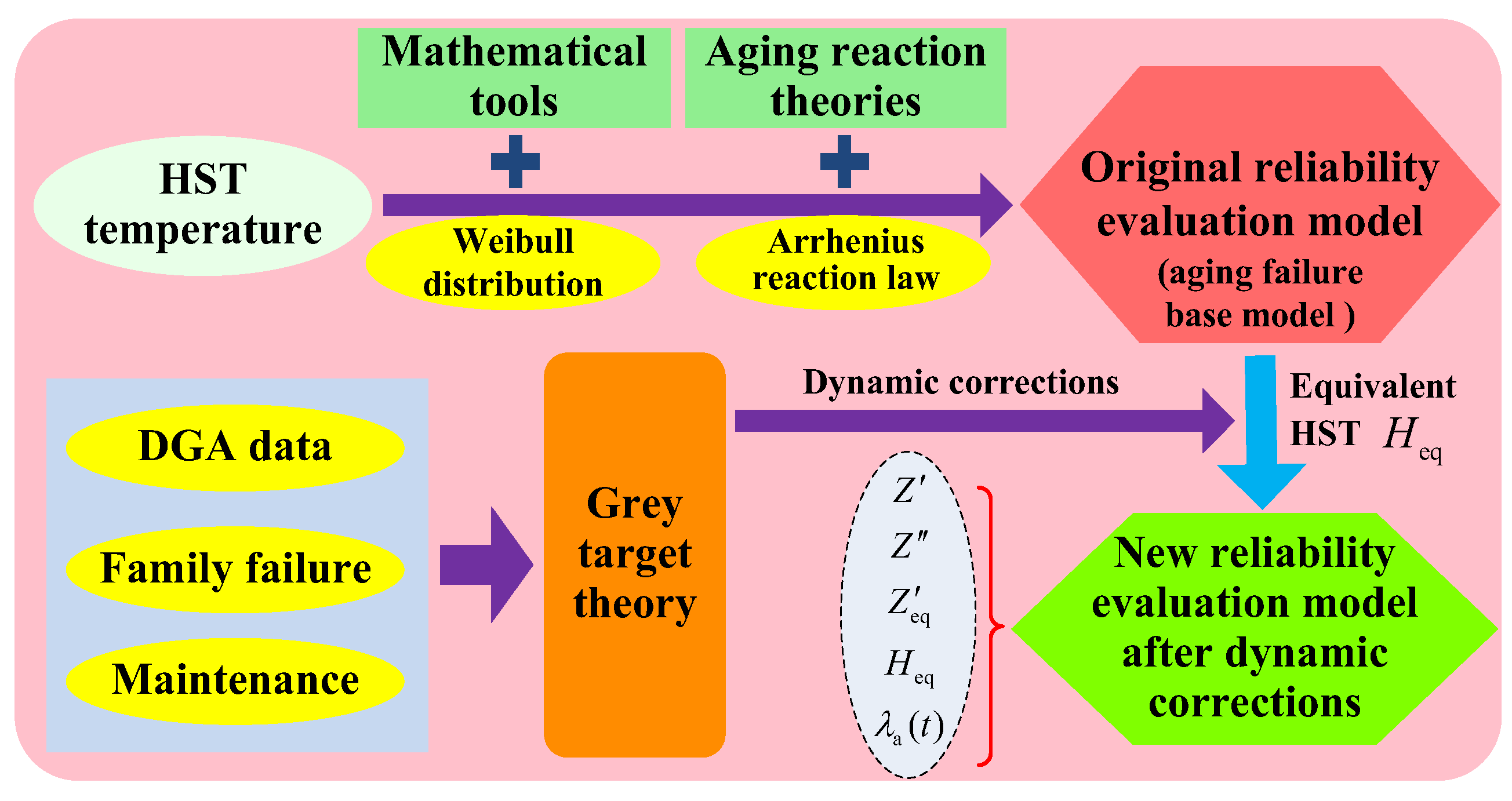
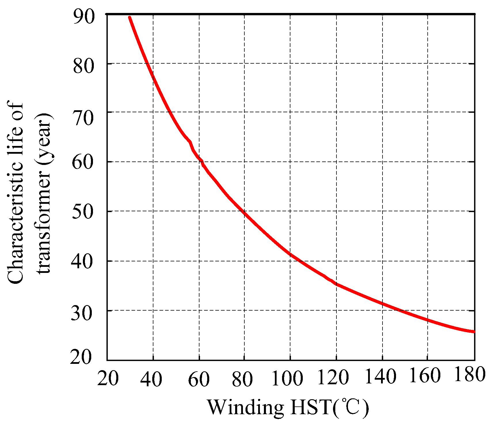
According to the Standard Operating Procedure of IEEE Standard C57.91-2011, as well as IEC Standard 60076-7, and combining with the Weibull distribution and Arrhenius reaction law, an HST-based ageing failure model as a static model was developed to describe the ageing process of transformer, in which the winding HST and transformer failure rate can be obtained, as well as the life expectancy of transformer can be further calculated. Compared to the traditional method of reliability assessment of transformer based on statistical theory, this static model has been developed which takes the individual differences of transformers into consideration, such that the failure rate level of the TOPIS can be better reflected and the result is more reliable.

(2)

In the traditional method, the characteristic parameters such as DP and VFF are used to reflect the reliability of transformer oil-paper insulation, which leads to some defects for the furfural, such as content is easily affected by external factors, difficult to be obtained, a long testing cycle, the model accuracy is not high. To avoid this, the DGA data, as the primary characteristic parameters, were employed in the grey target theory based model for dynamic corrections, such that the corresponding relation between the fault degree of TOPIS and the life expectancy of transformer was dynamically adjusted, the corrected life expectancy and life loss was obtained, and then the equivalent HST was achieved, and finally the dynamic correction of the static model can be realized. Besides, the age reduction factor was introduced, thus the model after the maintenance of TOPIS was considered so as to realize a more reliable diagnosis on transformer internal faults.

(3)

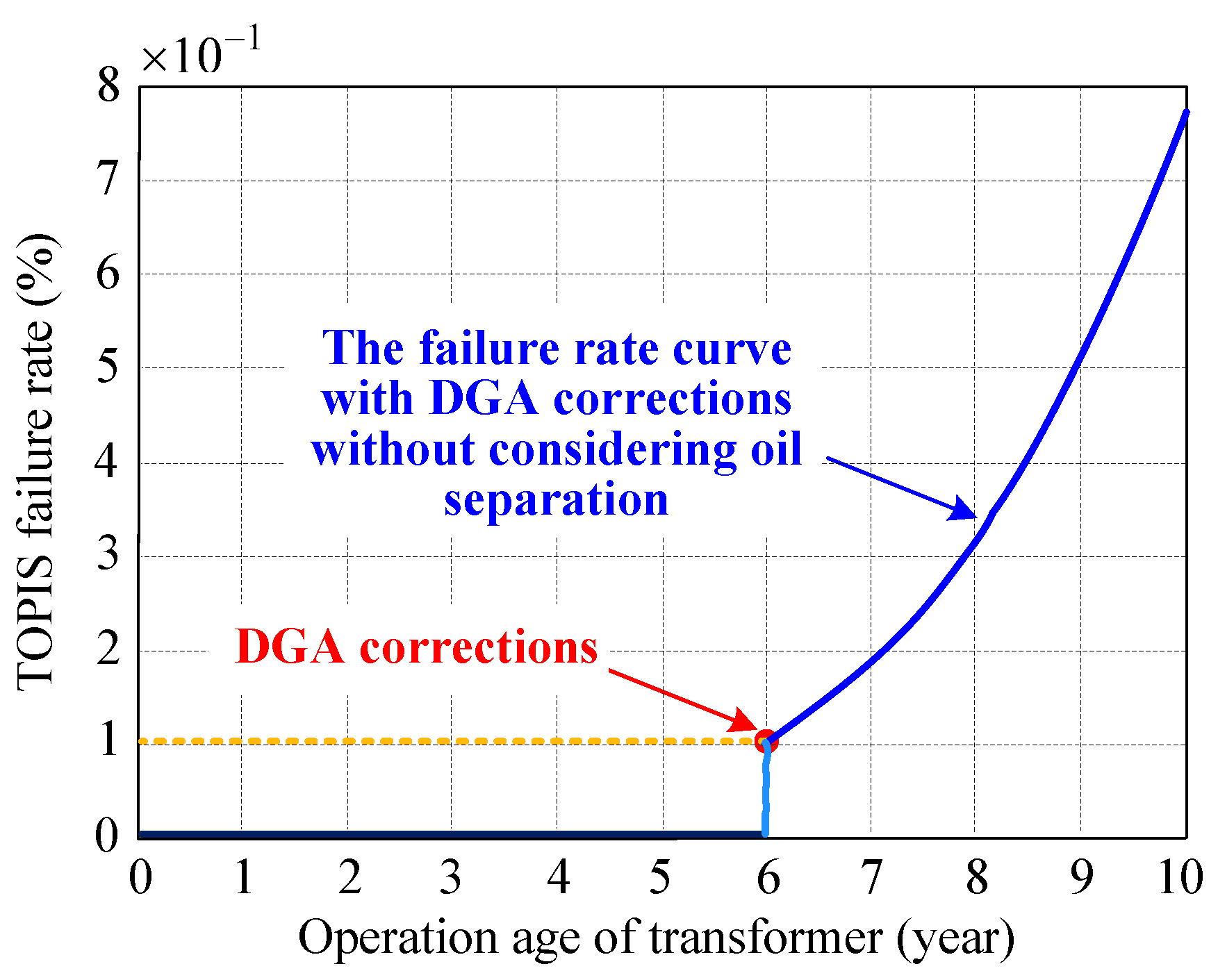
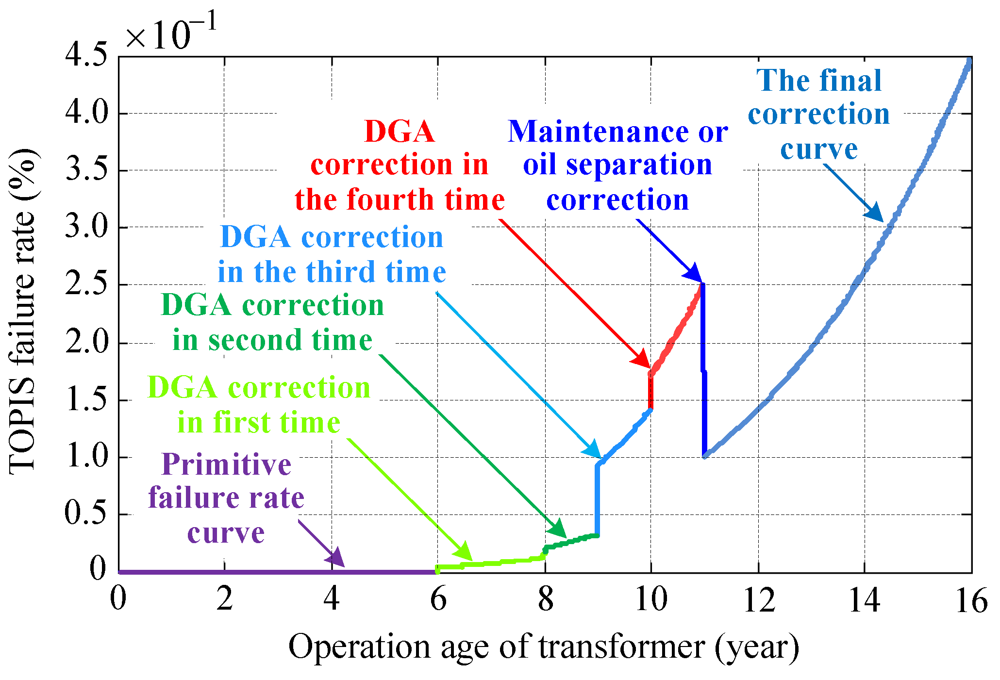
After the above dynamic corrections were introduced, the corrected failure rate curve was transformed into a dynamic ladder form, which would ensure that the failure rate and life prediction curves of the transformer are more consistent with the actual state of the transformer, thus the overall reliability assessment model can be properly adjusted according to the operating conditions of the evaluated objective, and a higher accuracy can be achieved.

(4)

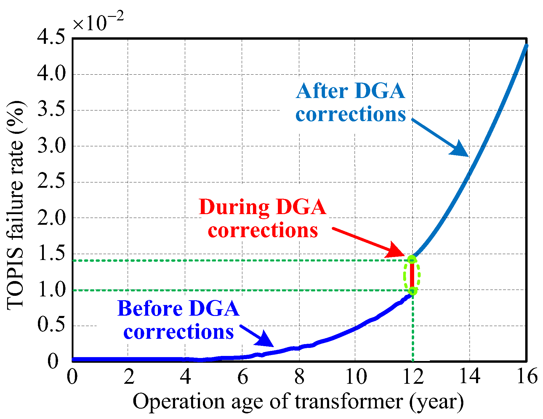
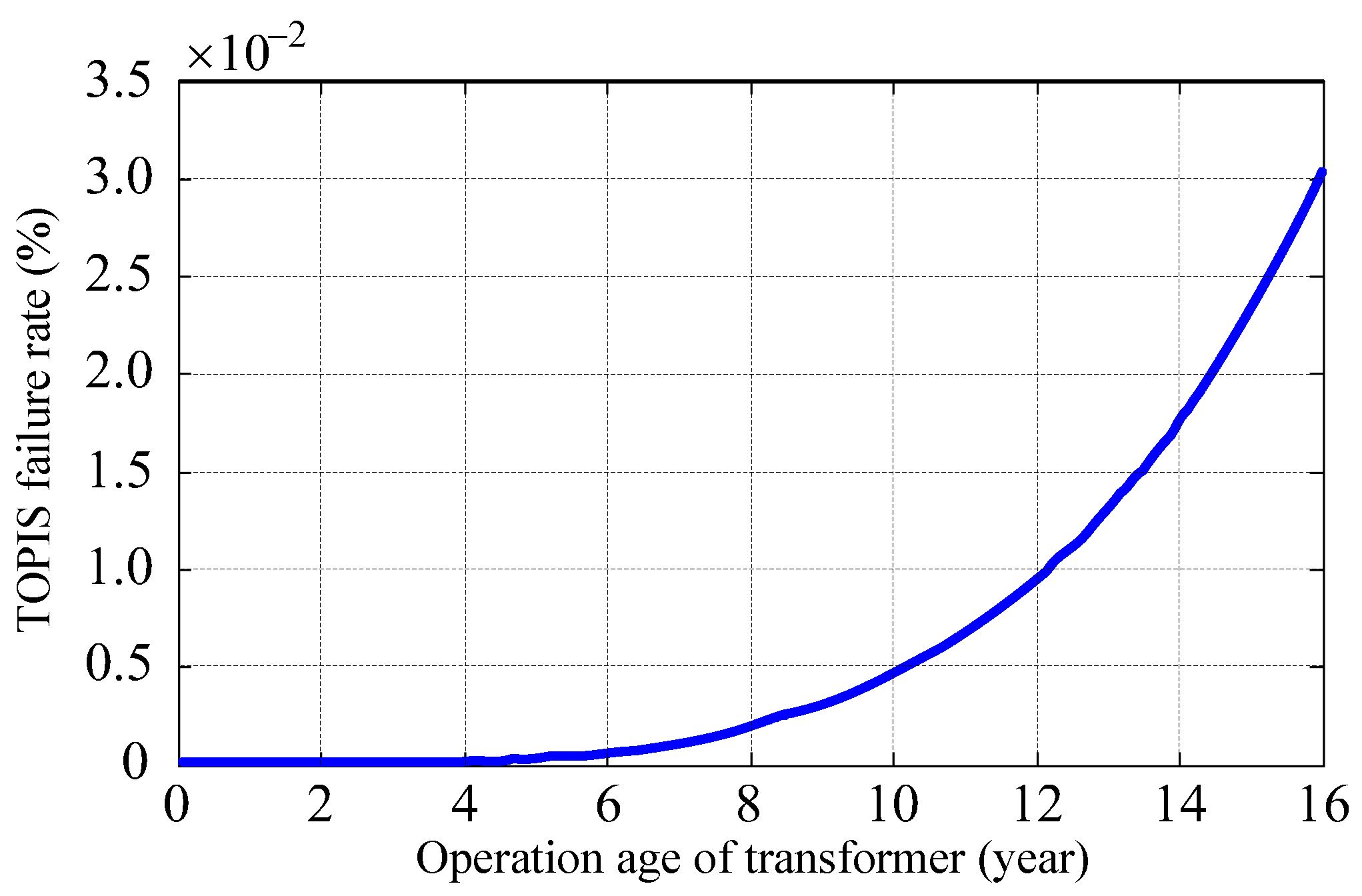
At last, a practical case study in China Southern Power Grid has been carried out. In this case, the actual data of a main transformer with 110 kV from the Jiangmen Power Supply Bureau were analysed to verify the validity of the built model. Here, according to the static ageing failure model, the failure rate of this transformer is only 0.01%, showed extremely low, and the corresponding life expectancy is 64.12 year, after it was put into operation for 12 years, this is mainly due to the load of the transformer is controlled at about 40%. After introducing dynamic corrections, the corrected life expectancy is 59.46 year via the DGA data analysis, as well as its corresponding corrected failure rate curve can be obtained. Owing to the good DGA data, the corrected failure rate is only 0.014%. This value is very low, showing that this transformer is in a good operating state and its detection data are very normal, which has been verified via verifying to the operation and maintenance personnel. This also verifies the correctness of the evaluation method proposed in this paper.

(5)

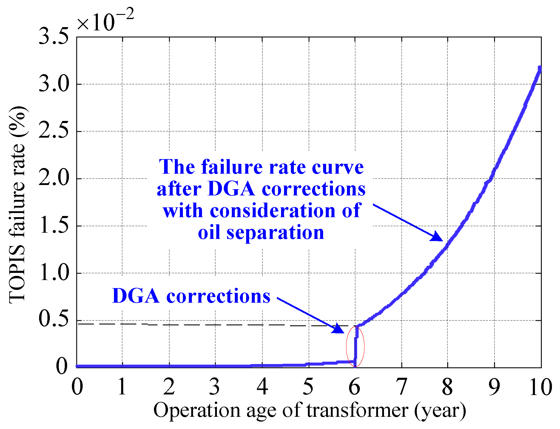
In addition, when the effect of maintenance is considered, the actual corrected life expectancy was 43.57 year, far higher than the value of the calculated 23.016 year when the maintenance effect is not considered. This also reflects that after the overhaul, the insulation fault of the transformer has been dealt with in time, the operation conditions have been improved, and the life expectancy loss has also been reduced. Besides, after considering the effect of oil filtering, the failure rate of the transformer operating to sixth years is 0.005%, much lower than the 0.1% before the correction. At this point, the corrected failure rate curve becomes a dynamic staircase-like piecewise curve, which shows that the failure rate of the transformer is updated with the operating state of the transformer. Hence, compared with usual method, the model developed in this paper can diagnose the internal fault of transformer more accurately and the evaluation values can better track and reflect the actual operating state of the transformer, thus the effectiveness and feasibility of the proposed model can be verified.

(6)

This paper also provides a scientific guidance for the decision-making of the planning, replacement, maintenance and technical transformation of the primary equipment in the power grid, as well as the routine maintenance operation of equipment and fault treatment analysis, and improves the efficiency of field work. In addition, the research results have strong applicability, which effectively reduces the difficulty of obtaining the characteristic parameters and improves the accuracy of the model, thus it is more conducive to the popularization and application of the model.

References

1. Faria, H.D.; Costa, J.G.S.; Olivas, J.L.M. A review of monitoring methods for predictive maintenance of electric power transformers based on dissolved gas analysis. Renew. Sustain. Energy Rev. 2015, 46, 201–209. [Google Scholar] [CrossRef]
2. Wang, C.; Wu, J.; Wang, J.Z.; Zhao, W.G. Reliability analysis and overload capability assessment of oil-immersed power transformers. Energies 2016, 9, 43. [Google Scholar] [CrossRef]
3. Godina, R.; Rodrigues, E.M.G.; Matias, J.C.O.; Catalão, J.P.S. Effect of loads and other key factors on oil-transformer ageing: Sustainability benefits and challenges. Energies 2015, 8, 12147–12186. [Google Scholar] [CrossRef]
4. Liao, R.J.; Zheng, H.B.; Grzybowski, S.; Yang, L.J.; Zhang, Y.Y.; Liao, Y.X. An integrated decision-making model for condition assessment of power transformers using fuzzy approach and evidential reasoning. IEEE Trans. Power Deliv. 2011, 26, 1111–1118. [Google Scholar] [CrossRef]
5. Mkandawire, B.O.; Ijumba, N.; Saha, A. Transformer risk modelling by stochastic augmentation of reliability-centred maintenance. Electr. Power Syst. Res. 2015, 119, 471–477. [Google Scholar] [CrossRef]
6. Lee, L.; Xie, L.J.; Zhang, D.; Yu, B.; Ge, Y.F.; Lin, F.C. Condition assessment of power transformers using a synthetic analysis method based on association rule and variable weight coefficients. IEEE Trans. Dielectr. Electr. Insul. 2013, 20, 2052–2060. [Google Scholar]
7. Ma, H.; Saha, T.K.; Ekanayake, C. Statistical learning techniques and their applications for condition assessment of power transformer. IEEE Trans. Dielectr. Electr. Insul. 2012, 19, 481–489. [Google Scholar] [CrossRef]
8. Bakar, N.A.; Abu-Siada, A. Fuzzy logic approach for transformer remnant life prediction and asset management decision. IEEE Trans. Dielectr. Electr. Insul. 2016, 23, 3199–3208. [Google Scholar] [CrossRef]
9. Secue, J.R.; Mombello, E.E.; Cardoso, C.V. Review of sweep frequency response analysis-SFRA for the assessment of winding displacements and deformation in power transformers. IEEE Lat. Am. Trans. 2007, 5, 321–328. [Google Scholar] [CrossRef]
10. Sica, F.C.; Guimarães, F.G.; Duarte, R.D.O.; Reis, A.J.R. A cognitive system for fault prognosis in power transformers. Electr. Power Syst. Res. 2015, 127, 109–117. [Google Scholar] [CrossRef]
11. Ma, H.; Saha, T.K.; Ekanayake, C. Predictive learning and information fusion for condition assessment of power transformer. In Proceedings of the 2011 IEEE Power and Energy Society General Meeting, Detroit, MI, USA, 24–29 July 2011; Volume 5, pp. 1–8. [Google Scholar]
12. Tenbohlen, S.; Coenen, S.; Djamali, M.; Müller, A.; Samimi, M.H.; Siegel, M. Diagnostic measurements for power transformers. Energies 2016, 9, 347. [Google Scholar] [CrossRef]
13. Zhang, Y.Y.; Liu, J.F.; Zheng, H.B.; Wei, H.; Liao, R.J. Study on quantitative correlations between the ageing condition of transformer cellulose insulation and the large time constant obtained from the extended Debye model. Energies 2017, 10, 1842. [Google Scholar] [CrossRef]
14. Yang, Y.; Xie, K.G.; Sun, X. Operating component failure rate analysis based on FTA for power system. Power Syst. Prot. Control 2009, 37, 134–137, 141. [Google Scholar]
15. Liao, R.J.; Xiao, Z.N.; Gong, J.; Yang, L.J.; Wang, Y.Y. Markov model for reliability assessment of power transformers. High Volt. Eng. 2010, 36, 322–328. [Google Scholar]
16. Rigatos, G.; Siano, P. Power transformers’ condition monitoring using neural modelling and the local statistical approach to fault diagnosis. Int. J. Electr. Power Energy Syst. 2016, 80, 150–159. [Google Scholar] [CrossRef]
17. Shah, A.M.; Bhalja, B.R. Discrimination between internal faults and other disturbances in transformer using the support vector machine-based protection scheme. IEEE Trans. Power Deliv. 2013, 28, 1508–1515. [Google Scholar] [CrossRef]
18. Bacha, K.; Souahlia, S.; Gossa, M. Power transformer fault diagnosis based on dissolved gas analysis by support vector machine. Electr. Power Syst. Res. 2012, 83, 73–79. [Google Scholar] [CrossRef]
19. Souahlia, S.; Bacha, K.; Chaari, A. MLP neural network-based decision for power transformers fault diagnosis using an improved combination of Rogers and Doernenburg ratios DGA. Int. J. Electr. Power Energy Syst. 2012, 43, 1346–1353. [Google Scholar] [CrossRef]
20. Shah, A.M.; Bhalja, B.R. Fault discrimination scheme for power transformer using random forest technique. IET Gener. Transm. Distrib. 2015, 10, 1431–1439. [Google Scholar] [CrossRef]
21. Hong, K.; Huang, H.; Zhou, J. Winding condition assessment of power transformers based on vibration correlation. IEEE Trans. Power Deliv. 2015, 30, 1735–1742. [Google Scholar] [CrossRef]
22. Jakob, F.; Dukarm, J.J. Thermodynamic estimation of transformer fault severity. IEEE Trans. Power Deliv. 2015, 30, 1941–1948. [Google Scholar] [CrossRef]
23. Dong, L.X.; Xiao, D.M.; Liang, Y.S.; Liu, Y.L. Rough set and fuzzy wavelet neural network integrated with least square weighted fusion algorithm based fault diagnosis research for power transformers. Electr. Power Syst. Res. 2008, 78, 129–136. [Google Scholar] [CrossRef]
24. Lee, B.E.; Park, J.W.; Crossley, P.A.; Kang, Y.C. Induced voltages ratio-based algorithm for fault detection, and faulted phase and winding identification of a three-winding power transformer. Energies 2014, 7, 6031–6049. [Google Scholar] [CrossRef]
25. Ghoneim, S.S.M.; Taha, I.B.M. A new approach of DGA interpretation technique for transformer fault diagnosis. Int. J. Electr. Power Energy Syst. 2016, 81, 265–274. [Google Scholar] [CrossRef]
26. Christian, B.; Gläser, A. The behavior of different transformer oils relating to the generation of fault gases after electrical flashovers. Int. J. Electr. Power Energy Syst. 2017, 84, 261–266. [Google Scholar] [CrossRef]
27. Abu-Siada, A.; Hmood, S. A new fuzzy logic approach to identify power transformer criticality using dissolved gas-in-oil analysis. Int. J. Electr. Power Energy Syst. 2015, 67, 401–408. [Google Scholar] [CrossRef]
28. Illias, H.A.; Xin, R.C.; Bakar, A.H.A. Hybrid modified evolutionary particle swarm optimisation-time varying acceleration coefficient-artificial neural network for power transformer fault diagnosis. Measurement 2016, 90, 94–102. [Google Scholar] [CrossRef]
29. Pandya, A.A.; Parekh, B.R. Interpretation of sweep frequency response analysis (SFRA) traces for the open circuit and short circuit winding fault damages of the power transformer. Int. J. Electr. Power Energy Syst. 2014, 62, 890–896. [Google Scholar] [CrossRef]
30. Jürgensen, J.H.; Nordström, L.; Hilber, P. Individual failure rates for transformers within a population based on diagnostic measures. Electr. Power Syst. Res. 2016, 141, 354–362. [Google Scholar] [CrossRef]
31. Mcnutt, W.J. Insulation thermal life considerations for transformer loading guides. IEEE Trans. Power Deliv. 1992, 7, 392–401. [Google Scholar] [CrossRef]
32. Wang, Y.Y.; Gong, S.L.; Grzybowski, S. Reliability evaluation method for oil-paper insulation in power transformers. Energies 2011, 4, 1362–1375. [Google Scholar] [CrossRef]
33. Feng, D.; Wang, Z.; Jarman, P. Evaluation of power transformers’ effective hot-spot factors by thermal modeling of scrapped units. IEEE Trans. Power Deliv. 2014, 29, 2077–2085. [Google Scholar] [CrossRef]
34. Wang, Y.Y.; Yang, T.; Tian, M. The relationship between DP, fracture degree and mechanical strength of cellulose Iβ in insulation paper by molecular dynamic simulations. Int. J. Mod. Phys. B 2013, 27, 631–640. [Google Scholar] [CrossRef]
35. Taheri, S.; Gholami, A.; Fofana, I.; Taheri, H. Modeling and simulation of transformer loading capability and hot spot temperature under harmonic conditions. Electr. Power Syst. Res. 2012, 86, 68–75. [Google Scholar] [CrossRef]
36. IEEE Working Group for Loading Mineral-Oil-Immersed Transformers. IEEE Guide for Loading Mineral-Oil-Immersed Transformers and Step-Voltage Regulators; IEEE C57.91-2011; IEEE: New York, NY, USA, 2012; pp. 1–123. [Google Scholar]
37. International Electrotechnical Commission (IEC). Loading Guide for Oil-Immersed Power Transformers; IEC Standard 60076-7—Power Transformers—Part 7, Committee Draft, 14/403/CD; IEC: Geneva, Switzerland, 2001. [Google Scholar]
38. Tsuboi, T.; Takami, J.; Okabe, S.; Inami, K.; Aono, K. Aging effect on insulation reliability evaluation with Weibull distribution for oil-immersed transformers. IEEE Trans. Dielectr. Electr. Insul. 2010, 17, 1869–1876. [Google Scholar] [CrossRef]
39. IEEE Std. IEEE Guide for Loading Mineral-Oil-Immersed Transformers; C57.91-1995; IEEE: New York, NY, USA, 1995. [Google Scholar]
40. Transformers Committee of the IEEE Power Engineering Society. IEEE C57.12.90-1993-IEEE Standard Test Code for Liquid-Immersed Distribution, Power, and Regulating Transformers and IEEE Guide for Short-Circuit Testing; IEEE: New York, NY, USA, 1993. [Google Scholar]
41. Gooch, J.W. Encyclopedic Dictionary of Polymers: Arrhenius Equation; Springer: New York, NY, USA, 2006; pp. 66–67. [Google Scholar]
42. Geng, N.; Yong, Z.; Sun, Y.X.; Jiang, Y.J.; Chen, D.D. Forecasting China’s annual biofuel production using an improved grey model. Energies 2015, 8, 12080–12099. [Google Scholar] [CrossRef]
43. Zeng, F.; Cheng, X.; Guo, J.C.; Tao, L.; Chen, Z.X. Hybridising human judgment, AHP, grey theory, and fuzzy expert systems for candidate well selection in fractured reservoirs. Energies 2017, 10, 447. [Google Scholar] [CrossRef]
44. Dinmohammadi, A.; Shafiee, M. Determination of the most suitable technology transfer strategy for wind turbines using an integrated AHP-TOPSIS decision model. Energies 2017, 10, 642. [Google Scholar] [CrossRef]
45. Awadallah, S.K.E.; Milanovic, J.V.; Jarman, P.N. The influence of modeling transformer age related failures on system reliability. IEEE Trans. Power Syst. 2015, 30, 970–979. [Google Scholar] [CrossRef]
Figure 1. Internal temperature characteristic curve of oil-immersed transformer. HST: hot spot temperature.
Energies 11 00249 g001
Figure 2. Flow chart of winding HST calculation.
Energies 11 00249 g002
Figure 3. The flow chart of dynamic correction.
Energies 11 00249 g003
Figure 4. Framework of the final reliability assessment model for the transformer oil-paper insulation system (TOPIS).
Energies 11 00249 g004
Figure 5. Average temperature curve of South China Jiangmen city in January from 1957 to 2013.
Energies 11 00249 g005
Figure 6. Load rate curve of main transformer (#2).
Energies 11 00249 g006
Figure 7. The temperature rise curve on 1 January, 2013.
Energies 11 00249 g007
Figure 8. Curve of expected life vs. the winding HST.
Energies 11 00249 g008
Figure 9. Failure rate curve of the TOPIS.
Energies 11 00249 g009
Figure 10. The curve of TOPIS failure rate after corrections. DGA: dissolved gas analysis.
Energies 11 00249 g010
Figure 11. The failure rate curve of TOPIS in its sixth year of operation without considerations of the influences of oil separation.
Energies 11 00249 g011
Figure 12. The curve of TOPIS failure rate in its sixth year operation period with considerations of the influences of oil separation.
Energies 11 00249 g012
Figure 13. The original failure rate curve of TOPIS.
Energies 11 00249 g013
Figure 14. Actual failure rate curve of the TOPIS.
Energies 11 00249 g014