Review

A Review of Experiments and Modeling of Gas-Liquid Flow in Electrical Submersible Pumps

McDougall School of Petroleum Engineering, The University of Tulsa, Tulsa, OK 74104, USA
*
Author to whom correspondence should be addressed.
Energies 2018, 11(1), 180; https://doi.org/10.3390/en11010180
Submission received: 18 October 2017 / Revised: 23 December 2017 / Accepted: 3 January 2018 / Published: 11 January 2018
(This article belongs to the Section I: Energy Fundamentals and Conversion)

Abstract

:
As the second most widely used artificial lift method in petroleum production (and first in produced amount), electrical submersible pump (ESP) maintains or increases flow rate by converting kinetic energy to hydraulic pressure of hydrocarbon fluids. To facilitate its optimal working conditions, an ESP has to be operated within a narrow application window. Issues like gas involvement, changing production rate and high oil viscosity, greatly impede ESP boosting pressure. Previous experimental studies showed that the presence of gas would cause ESP hydraulic head degradation. The flow behaviors inside ESPs under gassy conditions, such as pressure surging and gas pockets, further deteriorate ESP pressure boosting ability. Therefore, it is important to know what parameters govern the gas-liquid flow structure inside a rotating ESP and how it can be modeled. This paper presents a comprehensive review on the key factors that affect ESP performance under gassy flow conditions. Furthermore, the empirical and mechanistic models for predicting ESP pressure increment are discussed. The computational fluid dynamics (CFD)-based modeling approach for studying the multiphase flow in a rotating ESP is explained as well. The closure relationships that are critical to both mechanistic and numerical models are reviewed, which are helpful for further development of more accurate models for predicting ESP gas-liquid flow behaviors.

1. Introduction

The electrical submersible pump (ESP), as a high-efficiency downhole equipment for converting kinetic energy to hydraulic pressure head, has improved significantly since it was invented in the 1910’s by the Russian engineer Arutunoff. Globally, there are more than 100,000 ESP installations, making ESP the second most widely used artificial lift method in oil production, but the first based on the produced amount [1,2]. ESPs excel in producing crude oils at very high flow rate, but they have to be operated within a narrow application window. Gas involvement, changing production rate and high oil viscosity can greatly affect the ESP performance [3,4].
Previous studies showed that the presence of gas would cause ESP hydraulic head degradation. The flow behaviors inside ESPs under gassy conditions, such as pressure surging and gas pockets, further deteriorate ESP boosting pressure. Surging may result in vibrations and short service life, and gas pockets can severely limit liquid production rates [5]. Although handling gas-liquid mixture has gradually become common for ESPs, the physical mechanism of two-phase flow affecting ESP hydraulic performance is not well understood. The gas bubble formation, coalescence and breakup mechanisms inside ESPs, which affect the two-phase flow characteristics, are still unclear. Due to the compact and complex geometries of multistage ESPs, the visualization of internal flow structures and bubble movement is very difficult.
The main objective of this paper is to provide a comprehensive review of literature concerning experimental studies and modeling approaches for predicting ESP pressure increment under gas-liquid flow conditions. The review helps better understand the multiphase flow characteristics inside a rotating ESP, in order to develop mechanistic model to predict ESP boosting pressure under gassy flow conditions. Section 2 presents the fundamental concepts and definitions of a multistage centrifugal pump. Section 3 discusses the previous knowledge of ESP hydraulic performance and flow structures under gassy conditions observed from experiments. Section 4 is divided into four subsections. It begins with the empirical correlations, followed by one-dimensional two-fluid modeling approach. Then, the CFD-based (Computational Fluid Dynamics) modeling and mechanistic approaches are discussed. Finally, the closure relationships to make models solvable are evaluated in Section 5.

2. Boosting Pressure of Centrifugal Pump
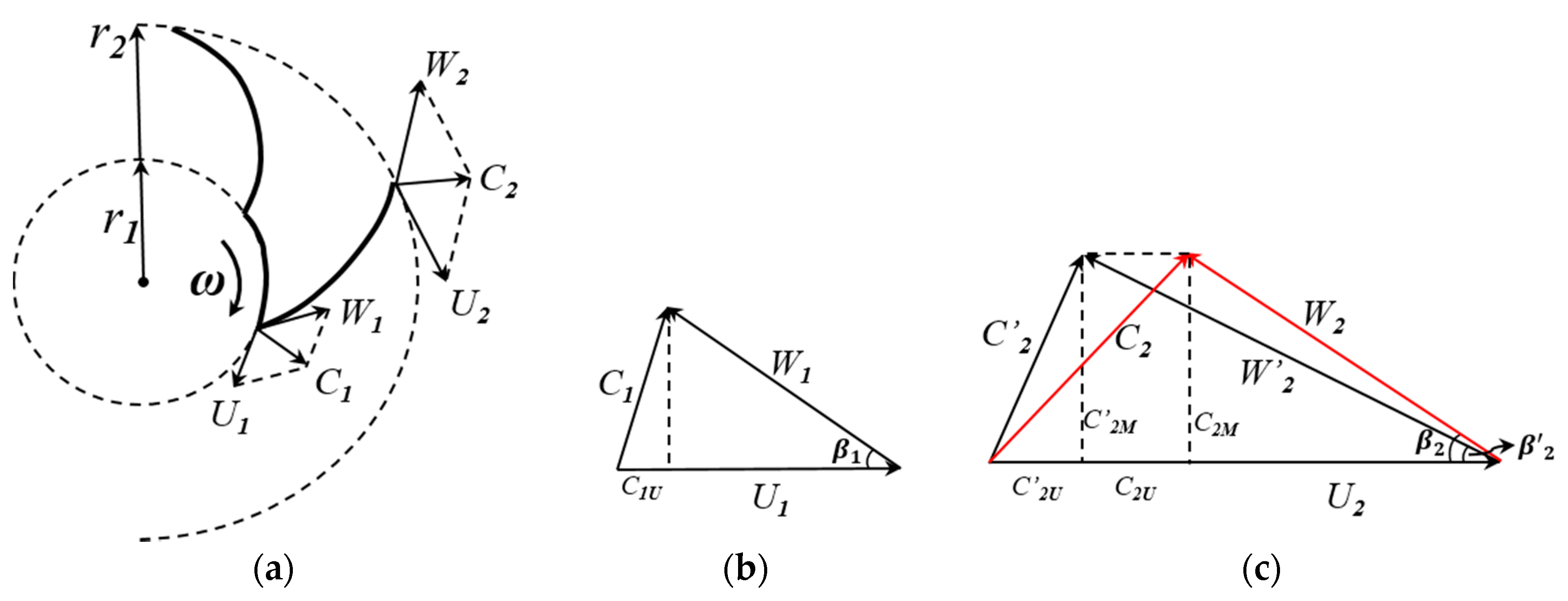
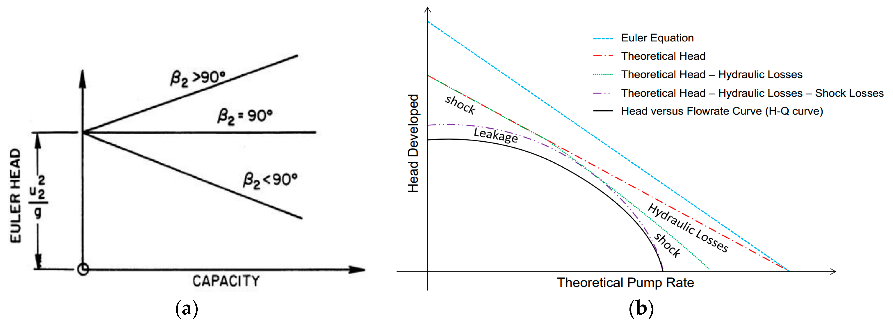
ESPs are widely used in petroleum industry to increase the hydrocarbon fluid production rates, especially for off-shore deep-water oil fields. Normally, multistage ESP is assembled in series (Figure 1a) with each stage comprising the rotating impeller and stationary diffuser (Figure 1b,c). In oil fields, the ESP system usually contains hundreds of stages to meet the boosting pressure requirement due to the great depth of reservoir. The impeller is the dominant part of ESP since it forces the fluid flow and adds kinetic energy to the fluids by spinning the blades. At the outlet of impeller, the main part of kinetic energy in the fluid is converted to pressure potential by diffuser vanes, which are fixed and work as the guiding channels for the impeller of the next stage.
As a type of centrifugal pumps, ESPs can be classified into three different categories: radial, axial and mixed types based on the dimensionless specific speed (NS). The non-dimensional NS is given by:
N S = Ω Q 1 / 2 ( g H ) 3 / 4
where Ω is the rotational speed (rad/s), Q is liquid flow rate (m3/s), g is local gravitational acceleration (m/s2), H is pump head (m). The pump industry uses a more practical expression for the specific speed NS as below:
N q = N q h 0.75
where N, q and h are rotational speed (rpm), flow rate (gpm) and pump head (ft), respectively. Based on Equation (2), centrifugal pumps are categorized into radial, mixed and axial types. The radial pumps usually fall in the range 500 < NS < 1800, while the mixed pumps can reach a maximum NS = 4500.
For a centrifugal pump, there are three important variables to characterize its hydraulic and mechanical performance, namely: pumping head (H), efficiency (η) and brake horsepower (BHP). Figure 2 below shows the typical pump performance curves provided in the product brochure, which are obtained experimentally using tap-water.
With the liquid flow rate increase, the ESP performance curves exhibit different trends. The horsepower and pumping head render a monotonic increasing and decreasing trend versus flow rate, respectively, whereas the efficiency is in a semi-quadratic relationship with the pump capacity. The best efficiency point (BEP) presented with the dashed line, corresponds to the highest efficiency of 68.9% at Q = 2700 bpd, N = 3500 rpm in Figure 2. It is an important parameter in characterizing the ESP overall performance. In this study, the main objective is to review different models in predicting ESP hydraulic boosting pressure under gas-liquid flow conditions.

2.1. Euler Head

For an ESP impeller, the velocity triangles at the intake and discharge are shown in Figure 3. All the variables are in International System of units (SI). The absolute velocity C can be decoupled into two components: relative velocity W and peripheral velocity U, which is calculated by U = Ω × r . The subscripts 1 and 2 denote the inlet and outlet of impeller, respectively. Here, W is relative to the impeller and C is relative to the global coordinate and is equal to the vector summation of U and W, e.g., C = W + U . In Figure 3c, C’2 is an ideal absolute velocity assuming infinite number of impeller blades, while C2 is the real absolute velocity at the impeller outlet.
According to the ideal conservation law of angular momentum in rotating centrifugal pump, the Euler head (HE) can be expressed as [6]:
H E = C 2 U 2 C 1 U 1 g = U 2 C 2 U U 1 C 1 U g
where C1U and C2U are the projection of absolute velocities at the impeller inlet and outlet to the direction of peripheral velocities. Applying the velocity triangle relationship in Figure 3, one can obtain:
H E = U 2 2 U 1 2 2 g + W 1 2 W 2 2 2 g + C 2 2 C 1 2 2 g
and:
H E = Ω 2 ( r 2 2 r 1 2 ) g Q Ω 2 π g h ( 1 tan β 2 1 tan β 1 )
where r is the radius of impeller, h is the channel height, β is the blade angle. If the fluids enter the impeller without pre-rotation, Equation (5) can be written as:
H E = Ω 2 r 2 2 g Q Ω 2 π g h tan β 2

2.2. Head Loss Mechanisms

As shown in Equation (6), the ideal Euler head HE is in linear relationship with liquid flow rate. In reality, pressure losses in the impeller, the diffuser, and losses from the interaction between them must be deducted from the ideal Euler head, including friction, shock and recirculation losses. Therefore, the actual pump head can be calculated by:
H = H E H f r i t i o n H s h o c k H l e a k a g e H r e c i r c u l a t i o n H d i f f u s e r H d i s k
Figure 4a shows the change of the ideal Euler head with the outlet blade angle β. Figure 4b shows the losses to the ideal head and the final H-Q curve of a centrifugal pump according to Equation (7). Friction loss becomes prominent at high flow rates. In contrast, leakage loss is more at relatively low flow rates. Shock loss takes place when the liquid flow rate differs from the designed flow rate. Table 1, Table 2, Table 3, Table 4 and Table 5 below discuss each pressure loss mechanism by presenting existing models that are available in literature.
Table 1 summarizes the studies on the friction losses inside a centrifugal pump impeller. Takacs [3] pointed out that friction losses progressively increase with liquid rate and are due to fluid friction in the impeller.
The mechanism of shock losses in centrifugal pump is still not well studied. Thus, only empirical correlations are available in the literature. Table 2 lists the existing prediction models of shock loss as implemented in the prediction models. Shock losses are negligible at the best efficiency point (BEP) of the pump, but increase at lower and higher liquid flow rates. They occur at the entrance and the exit of the impeller and are caused by sudden changes in the direction of flow [3].
As suggested by Tackas [3], the leakage losses represent the losses through the clearances between the rotating and stationary parts of the pump stage (at the impeller eye, through balancing holes, etc.), which decrease with increase of liquid rates. Table 3 below shows the calculation models available in literature.
In a rotating centrifugal pump, recirculation loss is interpreted as the dissipated fluid energy which is continuously obtained from the shaft due to adverse pressure gradient from the impeller inlet to outlet. As liquid flow rate decreases, the adverse pressure gradient increases, resulting more severe head loss due to fluid recirculation. Currently, the agreement has not been reached as for the definition of recirculation, which in turn a fully understanding in terms of recirculation loss mechanism is unavailable by far. However, the empirical correlations have been proposed in literature, as summarized in Table 4 below.
Sun and Prado [12,14,22] claimed that the diffuser loss is caused mainly by the friction on the diffuser walls. Table 5 presents the calculation formulae of diffuser losses that were implemented in the prediction models. Most equations are similar to the friction loss formulae in Table 1.
Disk friction losses, as Stepanoff [6] defined, are due to the contact between a rotating disk and fluid. Thus, additional power is consumed to keep the disk rotating since the viscous shear forces act on the disk surfaces [7]. Table 6 shows some of existing models of calculating disk friction losses in literature.
By deducting the pressure losses from Euler head in Equation (7), the real pressure increment of a centrifugal pump is obtained for single-phase flow. As can be seen in the Table 1, Table 2, Table 3, Table 4, Table 5 and Table 6, different pressure loss models are available in literature. A proper combination of these models may output an optimized estimation of pump performance. Yet, due to the empirical nature of these models, the universal validity of such combination to deduce the most appropriate prediction model is questioned. Thus, more and more researchers resort to numerical approaches to calculate the hydraulic performance and understand the complicated flow structures inside rotating ESPs.

3. Experimental Studies

The ESP boosting pressure depends on many hydraulic factors including pump geometry, fluid properties and multi-phase flow conditions. In recent years, with more and more installations of ESP in oil production systems, the effects of fluid viscosity and gas entrainment on ESP’s pressure boosting ability have been the focal areas of research interests.

3.1. Single-Phase Tests

For single-phase flow, ESP performance is sensitive to the fluid viscosity. With the increase of oil viscosity, ESP boosting pressure becomes lower corresponding to the same flow rate. By the same token, the flow rate through the ESP decreases corresponding to the same boosting pressure in ESPs. Ippen [25] conducted over 200 performance tests for oil viscosities up to 10,000 Saybolt Second Universal (SSU) on four variants of centrifugal pumps. The experimental results were summarized by plotting the ratio of oil head to water head, brake horsepower and efficiency against a Reynolds-type dimensionless number, based on which the general correction factors for specific speeds from 800 to 2200 were proposed to correlate pump’s boosting pressure under viscous fluid flow.
Hydraulic Institute provided a typical empirical approach with correction factors to estimate the conventional centrifugal pump boosting pressure for viscous liquid flow if the water performance were known. However, the accuracy of this approach was questioned by Gülich [19,20] and Li [26] since the experiments carried out by Hydraulic Institute were within a narrow range of the pump specific speeds. Unreasonable errors were found if extrapolation was beyond that range.
Stepanoff [6] proposed a similar Reynolds-type number by using only one correction factor to get the new H-Q curves if the water performance were known. A more general model based on the evaluation of viscous dissipation for disk and hydraulic frictions to predict the boosting pressure of centrifugal pumps was proposed by Gülich. The friction losses on disk and in flow passage, as the author claimed, were dominating factors impairing centrifugal pump’s ability to handle high viscosity fluids. Compared with available data, Gülich also pointed out that friction losses were affected significantly by pump geometry, fluid properties and thermal conditions. More recent experimental studies conducted by Amaral et al. [27] and Solano [28] further revealed that the Hydraulic Institute charts and empirical correlations available in literature were unable to give appropriate correction factors to predict the ESP boosting pressure for viscous oil flow. The discrepancies between experimental measurements and predictions by existing correlations or charts are discussed in Barrios et al. [29] and Banjar et al. [30].

3.2. Two-Phase Tests

The pioneering experimental studies conducted by Murakami and Minemura [31,32] investigated centrifugal pump performance with gas entrainment. By employing a semi-opened impeller pump with a transparent casing, they experimentally observed the behavior of entrained air bubbles. The decreasing total head of the pump caused by air admission and the work consumed for air delivery were reported. Since then, investigators have conducted more experimental measurements and mathematical modeling on centrifugal pump performance under gassy flow conditions. Experimental researches of ESP performance under gas-liquid flow conditions have been carried out extensively at the Tulsa University Artificial Lift Project (TUALP) in the past decades. Table 7 lists a summary of these studies.
As can been seen in Table 7, the previous experimental studies, which were conducted by Cirilo [33], Pessoa [35], Beltur [36], Duran [37], Zapata [38], Barrios [39], Gamboa [40], and Salehi [42] among others, covers a wide range of flow conditions. Cirilo built the experimental flow loops for testing ESP performance at the TUALP. Using water and air as the working fluids, he measured both the water and air-water performances of three different types of ESPs as a function of GVFs (the volumetric fraction of gas phase at the ESP inlet), intake pressure and rotational speeds. The obtained data indicated that the mixed type pumps were able to handle much higher GVFs (>30%) than radial type pumps (<10%). With necessary modifications of the same testing flow loops, Pessoa conducted experimental investigations of two-phase performance of ESP using a 22-stage GC6100 pump. By monitoring the stage-by-stage pressure increment, his results revealed that the ESP average behavior was significantly different from that observed per stage. Also, phenomena like surging and gas locking were observed and their boundaries were mapped. Additionally, a second region after pressure surging was observed in mapping test curves, where the slope of pressure increment versus flow rate changed again.
Using the same experimental flow loop of Pessoa, Beltur, Duran, Zapata and Salehi conducted extensive experimental measurements of ESP performance under both liquid- and gas-liquid flow conditions. Beltur focused on ESP performance deterioration with the presence of gas for varying intake GVFs and pressure. Data analysis revealed that the intake GVF is the most important factor affecting ESP boosting pressure under gassy flow. A higher deterioration of pumping head occurs at GVFs above 6%. Duran and Zapata developed empirical correlations for predicting the pressure increment across the stage and the flow regime boundaries. Zapata also carried out further measurements with a wide range of rotational speed to study its effects on the average efficiency of ESP. Salehi did similar measurements using a 14-stage TE2700 ESP, on which the effects of the stage number, intake pressure and fluid properties were investigated. It was found that ESP two-phase boosting pressure varied stage by stage only when the GVF exceeded a certain value, below which the deterioration was mild and independent of stage number. However, the degradation of pumping head became more prominent and affected by the stage number if the GVF reached a critical value, at which the pump boosting pressure of the downstream stage is better than upstream ones.
A typical testing result of ESP two-phase performance with pure water-air flow is shown in Figure 5 [40], including surging (Figure 5a) and mapping tests (Figure 5b). For surging test, the liquid flow rate is fixed, but gas flow rate or inlet gas volumetric fraction (GVF) varies. On the contrary, the liquid flow rate changes while the gas flow rate is fixed in mapping test. In Figure 5a, different curves correspond to different pump intake pressures. Obviously, the pump pressure increment declines non-linearly with the increase of inlet GVF. For mapping test results in Figure 5b, each curve corresponds to a different gas flow rate, which increases from the top to bottom curves. With a fixed gas flow rate, a sudden drop of pump stage pressure increment is observed when flow rate is reduced to a certain value.
A more recent experimental study regarding surfactant effect on ESP gas-handling ability and boosting pressure under gassy flow was conducted by Zhu et al. [44]. Surfactants are molecules with a hydrophobic and a hydrophilic part, and therefore they preferentially adsorb at the interface of continuous/dispersed phases. In the process, they reduce the interfacial tension [45]. Studies of surfactant effect on bubble/droplet formation in air/water or water/oil binary immiscible two-phase flows were carried out by Hu et al. [46], Omer and Pal [47]. Surfactant effect on liquid loading in gas well has been studied by van Nimwegen et al. [48,49], Ajani et al. [50,51]. Both reported a lower critical gas velocity at which liquid loading occurs, meaning that the surfactant presence helps prevent liquid loading in wells.
However, the studies on the surfactant effect on centrifugal pump performance under two-phase flow conditions are few. Zhu et al. [44] measured the ESP two-phase pressure increment with/without surfactant injection in the flow loop. The surfactant used in their study is isopropanol alcohol (IPA). The decline trend of normalize pressure (Np) in Figure 6a versus the intake GVF improves with surfactant injections, and the pressure surging phenomenon depicted by a sudden drop of ESP boosting pressure disappears. Figure 6b compares ESP H-Q performance curves under air-water flow with different IPA volumetric concentrations. A clear difference can be seen at low QL in terms of the stage pressure increment. Without IPA injection, the pressure increment drops to zero if QL becomes very low. But, the ESP performance improves significantly with surfactant presence.

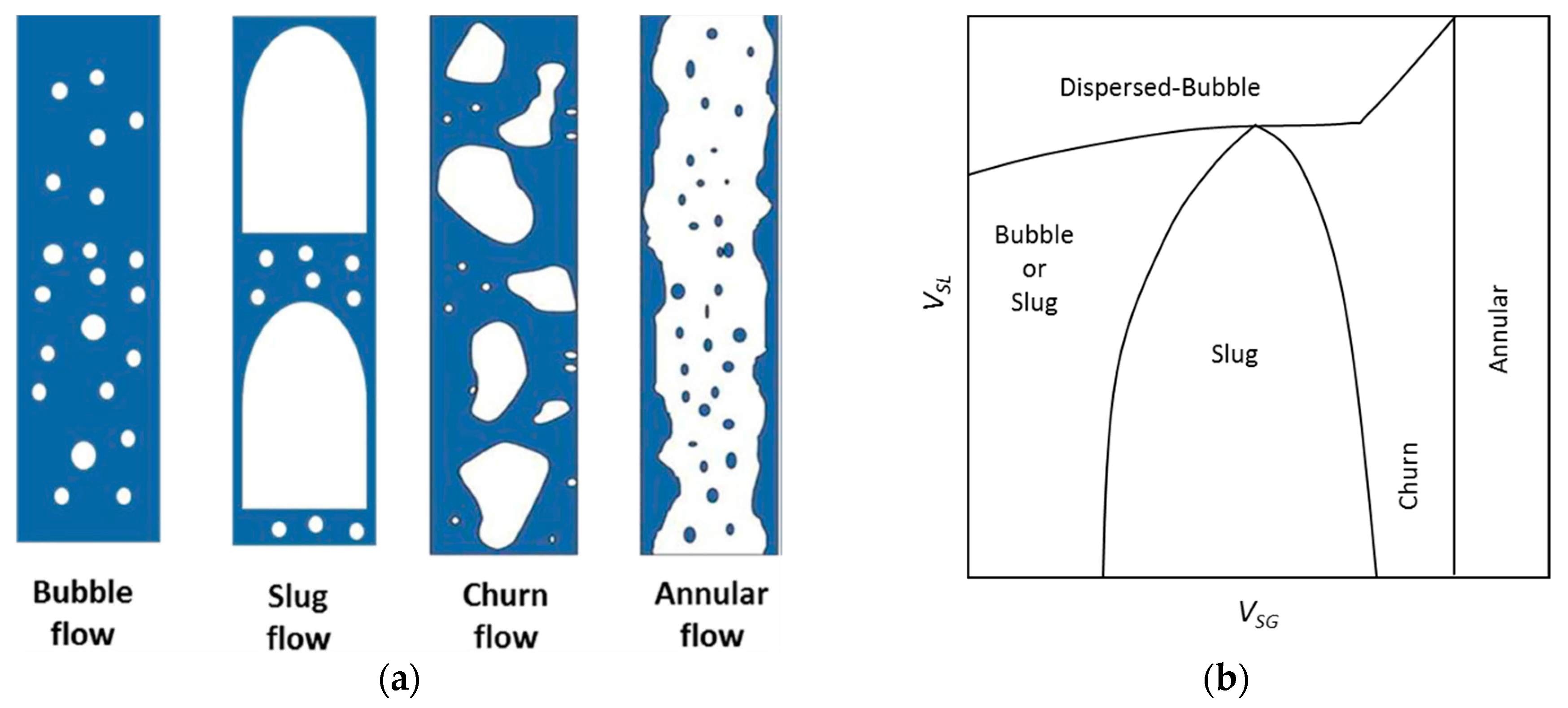
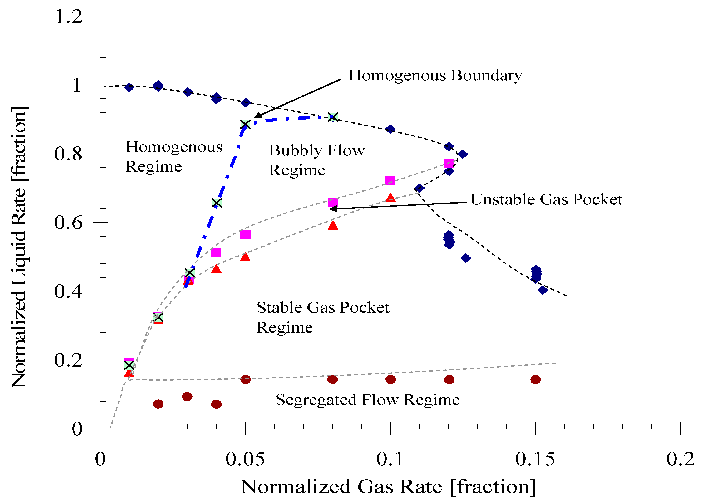
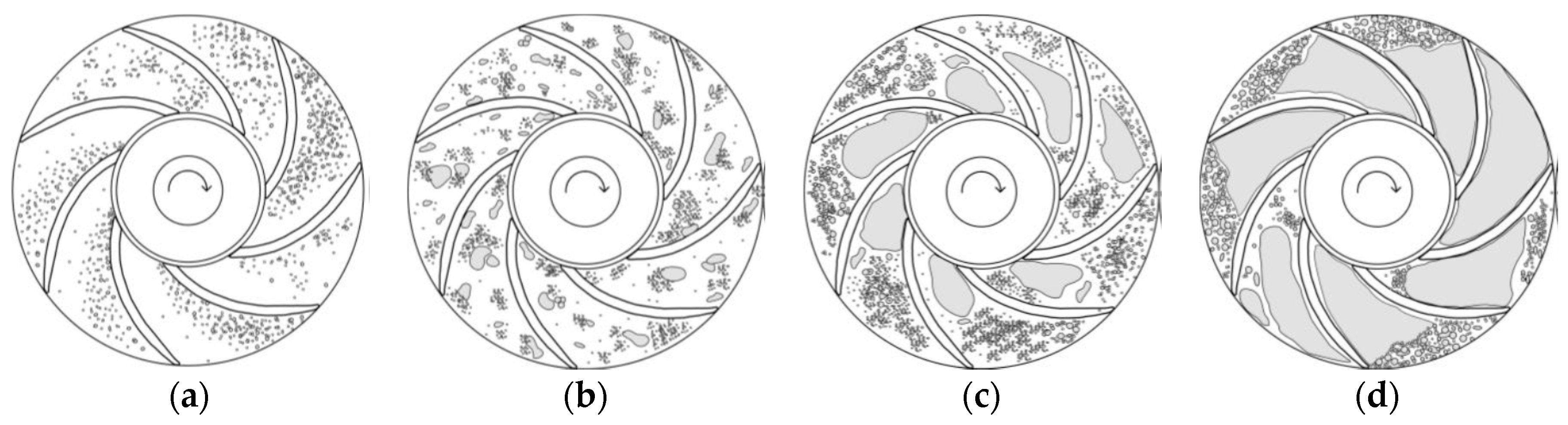
3.3. Flow Pattern Recognition

In multiphase pipe flow, flow pattern varies due to phase interaction and interfacial momentum transfer changes, which depend on fluid properties, flow rates and pipe geometry. Many studies on the recognition of flow patterns and their transition boundaries are available in literature [52,53,54]. Flow pattern is important to accurately predict the liquid holdup and pressure gradient in pipe flow. Take the upward gas/liquid flow in a vertical pipe for example, the main flow patterns are bubble, slug, churn and annular flows as illustrated in Figure 7a. Correspondingly, the flow pattern map showing the transition boundaries between different flow patterns is plotted in Figure 7b with the superficial velocities of gas and liquid as its coordinates.
The dispersed bubble flow prevails if the gas flow rate is low and the liquid flow rate is high, as shown in Figure 7a. For this flow pattern, the turbulence forces are high enough to breakup gas-phase into small bubbles and disperse them in the continuous liquid-phase [52].
When both gas flow rate and liquid flow rate are low, gas bubbles become larger and move upward in a zigzag path. The bubble flow regime may or may not exist depending on the pipe diameter. Confined by maximum lattice packing, the in-situ gas void fraction of bubble flow should be below 0.52 [55]. However, for a practical application, the maximum gas void fraction below 0.25 is commonly used for vertical co-current pipe flow.
Slug flow regime corresponds to the steady alternating flow of gas pockets (Taylor bubble) and liquid slugs [53] at even higher gas flow rates (see Figure 7b), where Taylor bubbles occupy the entire cross section of the pipe except for a thin liquid film on the wall. Slug flow can be considered as steady-state flow pattern since its slug length, frequency, translational velocity etc. are time-independent. However, a further increase of gas flow rates triggers the collapse of slugs and lead to an unstable flow that is described as the churn flow regime due to the large degree of turbulence in the flow [54].
Annular flow is characterized by extremely high gas flow rates and continuous gas core flowing upward with thin liquid film on the pipe wall. Due to high interfacial shear and drag force effects, the liquid droplets from the wavy interface between gas core and liquid film can be swept into the gas core, and pushed upward by the high-speed gas phase.
Several visualization studies have been conducted to observe multiphase flow structures/patterns inside a rotating centrifugal pump. Table 8 below lists the visualization experiments on flow patterns inside a centrifugal pump in literature. Most of these studies used transparent casing to visually observe the pump internal flow patterns. Starting with the original volute-type centrifugal pumps [31,32,56,57,58,59,60,61,62,63,64,65,66,67,68,69,70], they cover several research topics including flow pattern recognition, bubble movement visualization, mapping transition boundaries etc.
Murakami and Minemura [31,32] experimental study first investigated the gas entrainment effect on the hydraulic pump head of a centrifugal pump visually, and associated the degradation of pump performance with gas-liquid flow pattern inside the rotor. Using a transparent casing, Estevam [62] conducted the first visualization experiment of flow pattern recognition inside a rotating ESP impeller. Later visualization experimental work, conducted by Gamboa [40] presented similar observations as Estevam’s study, based on which the first flow pattern map with transition boundaries between different flow patterns inside an ESP was proposed. His work offers significant insight regarding how to characterize the flow patterns in an ESP quantitatively.
Among previous visualization experiments, two recent studies from Schäfer et al. [68] and Neumann et al. [69] are different from the others. They both used a new non-intrusive technique, the so called high resolution computed tomography (HireCT) to accurately measure the distribution of in-situ gas void fractions. Compared to the intrusive technique, the new measurement approach, as the authors claimed, can provide better image resolution of the gas void distribution and thus a higher measurement accuracy.
By visualizing the ESP internal flow, Barrios [39], Barrios and Prado [67] observed that bubbles enlarged when inlet GVFs increased and pump rotational speeds decreased. Such enlargement corresponding to the poorer pump performance indicated that bubble behaviors played a significant role in ESP’s ability of handling gas-liquid mixtures. In addition, visualization experiments also showed different flow patterns prevailing inside ESP channels at higher GVFs.
In Figure 8, λG denotes the intake GVF. It is evident that flow behaviors inside ESP impeller altered significantly with flow conditions. From Figure 8a,b, the GVF increase caused formation of larger bubbles and gas pockets, which in turn choked the flow passage for liquids and decreased the pump hydraulic head. Moreover, the flow patterns prevailing in ESP impeller at a specific value of λG, are comparable to that of gas-liquid two-phase flow in pipelines.
Similar as the gas/liquid pipe flow, Estevam [64] and Estevam et al. [71] categorized the flow patterns in a rotating ESP impeller as bubbly flow, transition flow, and elongated-bubble flow. A more thorough experimental study on flow pattern recognition of two-phase flow in ESP impeller was carried out by Gamboa [40], Gamboa and Prado [72]. Under a given flow condition, the typical flow pattern map from their visualization experiments is shown in Figure 9, where the curves denoted by different symbols represent the transition boundaries between flow patterns, including homogenous flow, bubbly flow, gas-pocket formation, and segregated flow. Figure 9 is important to understand the two-phase flow mechanisms in a rotating ESP. From the perspective of mechanistic modeling, each flow regime corresponds to the specific governing equations for flow characteristics, such as bubble size (db), in-situ gas void fraction (αG), slippage velocity (Vslip) between gas and liquid phases. With the flow pattern prevailing inside a rotating ESP determined, the governing equations based on mass and momentum conservations can be simplified.
Verde et al. [70] conducted visualization experiments on flow pattern recognition inside a rotating ESP impeller using high speed and resolution imaging technique. As shown in Figure 10, four different flow patterns were classified, including bubble flow (Figure 10a), agglomerated bubble flow (Figure 10b), gas pocket flow (Figure 10c) and segregated flow (Figure 10d). They observed that the intensity of pump performance degradation is directly influenced by the flow pattern within the impeller. The occurrence of the gas pocket flow pattern is linked to the intensification of the deterioration of pump performance and the appearance of operation instabilities. Moreover, the segregated flow patterns correspond to the severe performance degradation which makes the pump incapable of generating pressure.
Summarized by Verde et al. [70], the schematic representations of each flow pattern are shown in Figure 11 with intake GVF increasing from left to right. Due to the relatively small intake GVF, the homogenous flow regime is featured by tiny and evenly-dispersed bubbles inside impeller channels, as shown in Figure 11a. Under this regime, the bubbles are deemed to move together with liquid phase. Slippage between gas and liquid is small, meaning the in-situ αG is almost the same as λG.
As the intake GVF increases, the tiny bubbles are prone to collide and aggregate to form bigger ones, resulting in bubbly flow regime. In contrast to homogenous flow regime, the phase slippage between gas and liquid, shown by Figure 11b can no longer be neglected. Thus, depending on the intake GVF, the in-situ αG under bubbly flow becomes higher than λG. A further increase of GVF induces more severe collision and aggregation of bubbles so that the large gas pocket forms. This flow pattern is similar as slug/churn flow patterns in pipelines, which are featured by a gas core/pocket followed by a liquid slug. As shown in Figure 11c, the Taylor-bubble-like gas pocket forms near the suction side of ESP impeller, which occupies a significant portion of the impeller flow passage.
A relatively high gas flow rate and low liquid flow rate lead to the segregated flow pattern, similar to the annular/stratified flows in pipe. As it can be seen in Figure 11d, the elongated bubble expands and occupies the entire impeller length. For practical applications, the segregated flow pattern corresponds to gas-locking, an operational failure which gives null pump head and null flow rate [70].
As a direct observation of flow patterns inside the ESP impeller, visualization experiments can help reveal gas-liquid flow behaviors intuitively. However, the experimental facility needs special designs associated with necessary modifications on pump geometries, such as the removal of impeller hub and attaching the Pyrex glass on its top for visualized observation. Barrios [39] pointed out that the visualization of two-phase flow structures in a multistage ESP assembled in series was much more difficult. Thus, how to characterize the multiphase flow in ESPs has become a challenging topic. Although several technologies [68,69,73,74,75] to visualize the internal flows inside a centrifugal pump were discussed, they required some modifications on pump geometry and the implementation was difficult to carry out. It required mounting HireCT into the apparatus so that the internal flow structures could be visualized regardless of the opaque pump casing or volute. In addition, the data processing involved time-averaged rotation-synchronized CT scanning techniques, adding further complexity in analyzing the obtained experimental results.
Figure 12 shows the measurements using the HireCT technique by Schäfer et al. [68]. The horizontal axis denotes the inlet GVF and the vertical axis is the volumetric averaged in-situ αG in the rotating pump impeller. Clearly, there is a sharp αG increase at a GVF corresponding to the severe gas-pocket formation and pumping head degradation. The step change is between inlet GVF = 2.5% and 3.0%. As confirmed by Schäfer et al. observation, such change is due to the rapid flow pattern change from bubbly flow to intermittent flow.
The aforementioned experimental studies on ESP gas-liquid performance used tap water as the working fluid, while the gas phase was compressed air or nitrogen. Several recent experimental studies focusing on ESP gas-handling ability under viscous fluid flow were conducted by Trevisan [41], Trevisan and Prado [76], Banjar et al. [30], and Paternost et al. [77]. Using a visualization prototype built from original ESP components and with minimal geometrical modifications, Trevisan [41], Trevisan and Prado [76] conducted experiments to investigate the viscosity effect on liquid/gas two-phase flow through ESP. The authors identified four liquid/air flow patterns inside the impeller channels: agglomerated bubble, gas pocket, segregated gas and intermittent gas flows. It was concluded that the agglomerated bubble flow is responsible for pressure surging phenomenon, which is the initiation of pump head deterioration due to gas entrainment. The authors also observed that the increase in viscosity caused surging to occur at relatively lower inlet GVFs. Similar experimental observations were made by Banjar et al. [30]. Paternost et al. [77] further investigated the performance of a centrifugal pump handling single-phase viscous liquids and analyzed the impact of free gas entrainment. They concluded that the degradation of pump head was due to the stagnation of large gas-pocket formation, which became worse with the increase of liquid viscosity. An empirical correlation similar to the dimension analysis procedure in Solano [28] was proposed to correlate ESP pressure increment under two-phase flow conditions accounting the inlet GVF and fluid viscosity.

4. Modeling Approaches

In this section, several empirical correlations for calculating centrifugal pump performance under gas/liquid two-phase flow are reviewed. Although empirical correlations are much easier to implement compared to other numerical or mechanistic models, the application range is rather limited. With this consideration, the more sophisticated one-dimensional two fluid models coupled with interfacial momentum transfer mechanisms are discussed. The 3D CFD simulations, based on the conservation laws of mass and momentum, can provide detailed numerical results in terms of flow structure, phase distribution and slippage etc. However, CFD simulations for multiphase flow, which usually demand high computational cost, are not as reliable or robust as for single-phase flow. Furthermore, both one-dimensional two-fluid model and CFD-based numerical model are extremely sensitive to the closure relationships, such as bubble size, drag force model and other interphase momentum transfer terms, etc. Thus, the mechanistic models rooted in physics, including flow pattern, mass and momentum conservation equations, have become a new direction for developing the best prediction model of boosting pressure in ESPs with gas involvement.

4.1. Emperical Correlations

The first empirical correlation based on experimental data of ESP pressure degradation due to free gas entrainment was proposed by Turpin et al. [78]:
H m = H exp ( q g q l ( ( 346430 ( C 1 p i n ) 2 ) q g q l 410 C 1 p i n ) )
where, Hm is the head of ESP with gas/liquid flow (ft); H is the single-phase pump head (ft); qg and ql are gas and liquid flow rates (bpd), respectively; pin is pump intake pressure (psi); C1 = 0.145 is a unit conversion constant. As the authors claimed, a critical constraint of stable flow condition inside ESPs should be applied to this model so as to achieve a reasonable prediction accuracy. Thus, another empirical correlation to distinguish the stable/unstable flow boundaries are given as below:
ϕ = 2000 ( q g / q l 3 p i n )
The stable flow condition corresponds to ϕ < 1, which is the recommended application range of Equation (8).
Romero [34] established a multiphase head model for the type of mixed flow pumps based on Cirilo’s [33] experimental data:
H m H max = ( 1 q l d q d max ) ( a ( q l d q d max ) 2 + q l d q d max + 1 )
where Hmax is the shut-in pump head in ESP; qld is the dimensionless liquid flow rate, a ratio of the intake liquid flow rate to the open flow rate (OFR). The application range for Equation (10), as pointed out by the authors, is dispersed bubble flow or low degradation of ESP performance:
a = 2.902 λ G + 0.2751
q d max = 1 2.2035 λ G
To extend the application range of above two empirical correlations, Duran and Prado [79] presented models for the mild and severe head degradations in ESPs, which correspond to bubbly and elongated bubble flow regimes:
Δ p m = { ( 1 α ) ρ l H q l 1 α + α ρ g H q g α 0.47075 0.21626 ln ( q g ( 1 α ) q max )
where Δpm is the pressure increment of single stage ESP with gas/liquid flow (psi), α is the in-situ gas void fraction. Equation (13) is applied to bubbly flow and elongated bubble flow, respectively. A closure relationship is presented below to solve for α in above equations:
q g ( 1 α ) q max = { ( 0.843 ρ m ρ l + 0.85 ) ( q l ( 1 α ) q max ) 1.622 q l ( 1 α ) 1.6213 q max 0.435
Similarly, Equation (14) corresponds to Equation (13), which can be used to calculate the in-situ gas void fraction and then the pressure increment in ESP with gas presence can be obtained accordingly. Although the application range of Equations (13) has been extended compared to Equation (10), its formulation is only based on the experimental data from a single ESP geometry without any validation against different pump models. Thus, its general validity is questioned due to its empirical nature.

4.2. One-Dimension Two-Fluid Modeling

Zakem [80] first developed a mathematical model using a one-dimensional control volume method to analyze gas bubbles and liquid interaction for straight blade impellers. Furuya [81] developed a similar analytical model by incorporating the pump geometry, void fraction, flow slippage, and the flow regime but neglecting the compressibility and condensation effects. The basic formula in Furuya study is given by:
m ˙ l 2 ρ l ( d n ) 2 1 1 α ( 1 1 α d α d s 1 d n d ( d n ) d s ) + m ˙ g 2 ρ g ( d n ) 2 1 α α 2 ( 1 α d α d s + 1 d n d ( d n ) d s ) + ρ l 2 [ ( m ˙ g ρ g α d n ) 2 ( 1 α d α d s + 1 d n d ( d n ) d s ) + ( m ˙ l ρ l ( 1 α ) d n ) 2 ( 1 1 α d α d s 1 d n d ( d n ) d s ) ] = ( ρ l ρ g ) ( 1 α ) r ω 2 sin β cos γ 3 8 C d r b ρ l ( m ˙ l ρ l ( 1 α ) d n m ˙ g ρ g α d n ) 2
m ˙ l and m ˙ g are the mass flow rates of liquid and gas. s is the streamline coordinate. n is the coordinate normal to the streamline coordinate s. β is the angle between relative flow velocity and circumferential direction. γ is the angle between the radial direction and the stream surface. Cd is the drag coefficient. rb is the bubble radius. Comparing with experimental data in literature, the model predictions were within the relative average error band of ±30% for GVF <20%, and ±50% for GVF >30%.
Sachdeva et al. [82,83] conducted a comprehensive investigation of two-phase flow in ESPs with air/water and diesel/CO2 mixtures. A dynamic five-equation, one-dimensional, two-fluid model accounting for pump geometry, intake pressure and GVF, fluid properties, was developed and verified to predict ESP boosting pressure. The basic equations of Sachdeva model are presented below.
The mass balance equations are:
d ( α G ρ G W G r sin β ) d s = 0
d ( ( 1 α G ) ρ L W L r sin β ) d s = 0
where r is radius in ESP, WG and WL are the mass flow rates of gas and liquid, respectively.
The momentum balance equations are:
α G ρ G V R , G V R , G s = α G P s + α G ρ G r ω 2 r s F W , G + F i + F v
( 1 α G ) ρ L V R , L V R , L s = ( 1 α G ) P s + ( 1 α G ) ρ L r ω 2 r s F W , L F i F v
where VR,G and VR,L are the radial components of gas and liquid absolute velocities, respectively. FW,G and FW,L are the friction forces of gas and liquid against the channel walls per unit volume of fluids. Fi is the interfacial friction force between gas and liquid per unit volume. Fv is the virtual mass force per unit volume.
Minemura et al. [84] also studied the performance of centrifugal pumps in the nuclear industry under air-water two phase flow conditions with a low inlet GVF (<10%). Based on energy change in the flow from the rotating impeller to the stationary volute, a 1D, two-fluid model considering fluid viscosity and air-phase compressibility in a rotating impeller was proposed. This model can be solved numerically with a prediction error of ±20% of the related flow capacity. However, both Sachdeva et al. and Minemura et al. models are valid only under a narrow application range or specific experimental conditions. Compared to Sachdeva model, the major difference in Minemura et al. model is that the momentum balance equations are based on the relative velocities of gas/liquid rather than the radial components of the absolute velocities, which are given as:
α G ρ G W G W G s = α G P s + α G ρ G r ω 2 r s F W , G + F i + F v
( 1 α G ) ρ L W L W L s = ( 1 α G ) P s + ( 1 α G ) ρ L r ω 2 r s F W , L F i F v
Based on Sachdeva et al. and Minemura et al. one-dimensional two-fluid models, Sun [12,22] developed a new two-phase model including a set of one-dimensional mass and momentum balance equations for predicting ESP performance. He also improved analytical models for wall frictional losses and shock loss, as well as new correlations for the drag coefficient. The general momentum balance equation along the streamlines is given by:
d p d r | s t r e a m l i n e = [ ρ p W p d W p d r + ρ p Ω 2 r + ( d p d s ) f , p d s d r M p , s α p d s d r ] s t r e a m l i n e
where the subscript p is g or l for gas or liquid phase, respectively. And Mp,s is the interfacial momentum transfer term. Eliminating the pressure increment term at the left hand side in Equation (24), the combined momentum balance equation can be expressed as
ρ l W l d W l ρ g W g d W g = ( ρ l ρ g ) Ω 2 r d r + ( ( d p d s ) f , l ( d p d s ) f , g ) d s M l , s 1 α l α g d s
Applying a finite differencing algorithm, a preferred numerical scheme [85], to solving this model, a good agreement of pump performance curve, αG distribution, surging and gas lock conditions against correspondent experimental measurements was obtained. Although many studies for modeling ESP performance under gassy conditions were conducted, mechanistic modeling is still needed due to the over-simplification and assumptions or narrow application ranges of the existing models.

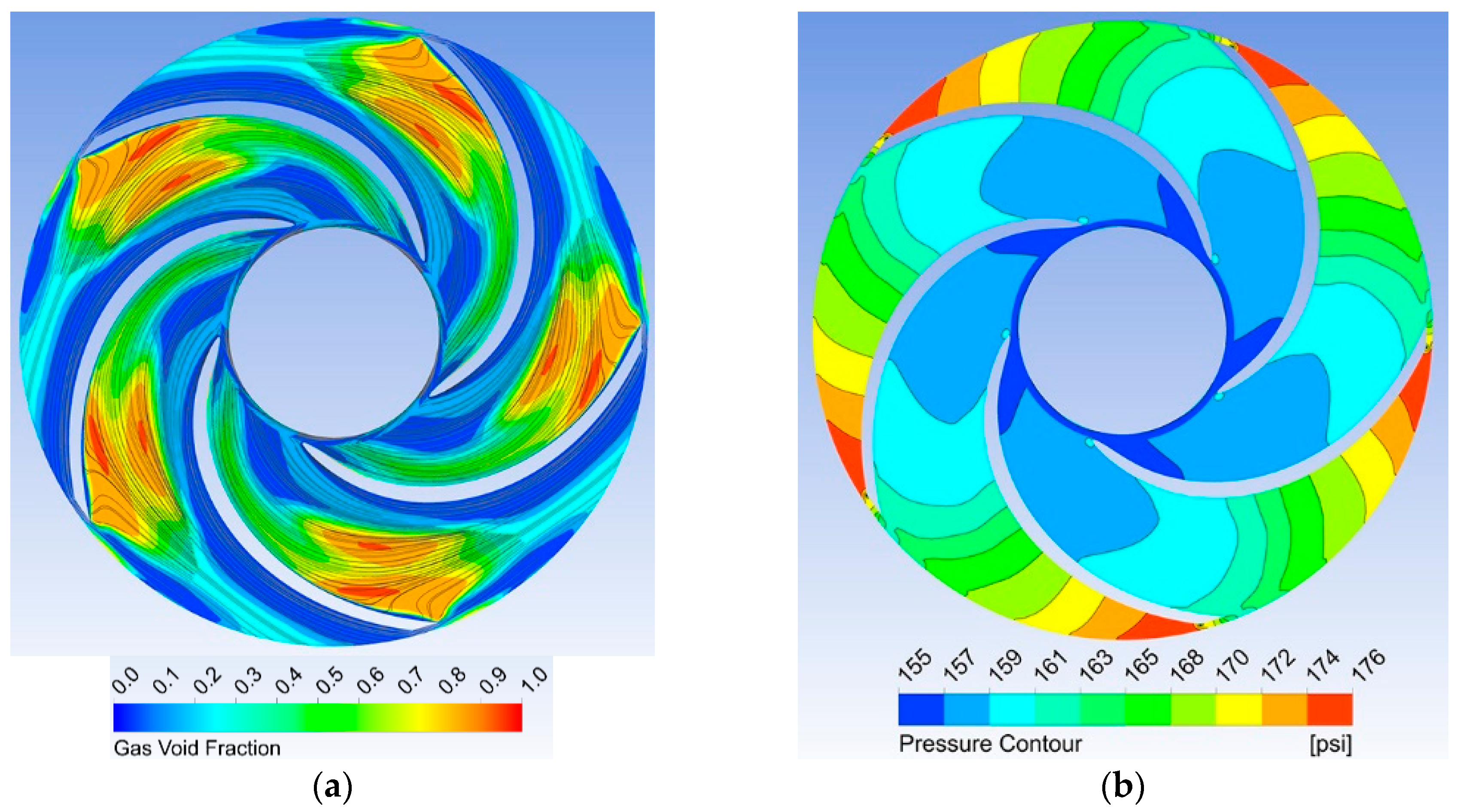
4.3. Three-Dimension Computational Fluid Dynamics (CFD)

With the advances of computer technology, computational fluid dynamics (CFD) becomes a more and more powerful tool to study centrifugal-pump performance under single-phase and multiphase flow conditions. Due to complicated ESP geometries, it is difficult to investigate the internal velocity and pressure fields experimentally. However, CFD offers an alternative way to simulate the complex internal flow structures. A centrifugal pump consists of an impeller rotating at a set angular velocity and a volute which is stationary. For an ESP, the rotating and stationary parts are the impeller and diffuser, which are accommodated in the rotating and stationary computational domains in CFD, respectively.
Using a 3D CFD code with the frozen-rotor interface model, the internal flow inside centrifugal pumps can be simulated, including velocity and pressure fields [86,87,88] as well as flow recirculation and separation [89,90]. The frozen-rotor model is considered as steady-state simulation because it holds the rotating and stationary parts in two separate reference frames. Some transient simulations were conducted using the sliding-mesh technique to investigate the dynamic flow structures in centrifugal pumps [91,92,93,94]. Gonzalez et al. [91] performed numerical simulations of unsteady flow in a single-phase centrifugal pump, considering impeller-volute interaction. By solving viscous, incompressible Navier-Stokes (N-S) equations with the sliding mesh technique, the unsteady flow behavior inside a centrifugal pump due to impeller-volute interaction was captured. A relationship between the global variables, such as torque, as a function of impeller relative position, secondary flow in volute, etc., was obtained numerically. This approach was successful in predicting the dynamic interaction between impeller and volute. Huang et al. [93] studied unsteady flow and pressure fluctuations due to interaction between impeller and diffuser vanes by the sliding mesh technique. His study confirmed that the global variables are primarily affected by impeller blade passing frequency.
In addition to designing turbomachinery, CFD can help engineers study the viscosity effects on centrifugal pump performance. Shojaeefard et al. [95,96] conducted both experimental study and numerical simulation of a centrifugal pump handling viscous fluids. The authors stated that a good agreement between simulation and experimental data was obtained by solving the steady state Reynolds-averaged Navier–Stokes (RANS) equations with Shear Stress Transport (SST) k-ω turbulence model. Using the same pump geometry, Sirino et al. [97] and Stel et al. [98] performed numerical investigations of viscosity effects on single-stage and three-stage ESPs, respectively. Similar numerical methodologies were used in their work including SST turbulence model with transient rotor-stator techniques. Both simulation results matched experiments well under a wide range of fluid viscosity. Stel et al. [98,99] pointed out that CFD simulated boosting pressure with multistage ESP geometry agreed with experimental results better than that with a single-stage geometry. The phenomenon of rising head with moderate increase of fluid viscosity was studied by Li [100]. By implementing the standard k-ε turbulence model and non-equilibrium wall function into RANS equations, the author confirmed that the rising pump head was due to the transition from hydraulically rough regime to hydraulically smooth regime. Zhu et al. [84] solved a set of 3D, steady-state RANS equations with standard SST turbulence model using the commercial CFD solver ANSYS CFX by employing the frozen-rotor technique. Their results matched correspondent experimental data well.
CFD has also been used to simulate pump performance with gas involvement, such as cavitation phenomenon [101,102], and free-gas entrainment flow [103,104,105]. Unlike single-phase simulations, the two-phase simulation requires the solution of conservation equations of mass, momentum and energy for the continuous and dispersed phases. Meanwhile, another set of constitutive equations, for describing the interphase interactions, such as interfacial momentum/heat transfer, need to be solved simultaneously.
Minemura and Uchiyama [106] solved 3D momentum equations with a finite-element method to predict gas/liquid flow behavior in a rotating centrifugal pump impeller. Tremante et al. [107] numerically studied gas/liquid flow through a cascade axial pump by CFD simulation. Coupled with a modified k-ε turbulence model by considering the viscosity of the liquid phase and the compressibility of the gas phase, the gas/liquid distributions versus different attack angles were obtained. Caridad et al. [108,109] studied ESP impeller performance handling water/air mixtures using CFD simulation. Applying two fluid models in 3D CFD simulations, the pressure and velocity fields, as well as the gas phase distributions (Figure 13) were obtained. The gas pocket near the impeller blade was also identified and compared with experimental observations.
The sensitivity analysis on GVF and bubble diameter indicated that ESP performance deteriorated with GVF and bubble diameter increase. Barrios [39], Barrios et al. [103] conducted multiphase CFD simulations on a single-stage ESP impeller with the new models of bubble size and drag coefficient predictions. Their simulations agreed with laboratory visualization images of streamlines and gas-accumulation zones. Qi et al. [110] designed ESPs for geothermal application with high-temperature gas-liquid two-phase flow. Using CFD simulations, the designed mix-type centrifugal impeller and diffuser were optimized for better gas-handling and higher efficiency within a wide range of production rate. Zhu and Zhang [104] conducted multiphase CFD simulations on a three-stage ESP with each stage comprising of an impeller and a diffuser. Comparing to experimental measurements, their work revealed that bubble size was a critical factor affecting ESP performance under gassy conditions. A new bubble size prediction model was later proposed in Zhu and Zhang [105] based on CFD simulations. They also predicted the in-situ gas void fraction (αG) with a mechanistic model and validated the results with numerically simulated values (Zhu and Zhang [90]). A typical CFD simulation result of gas/liquid flow inside a rotating ESP from their studies is shown in Figure 14 below.
Multiphase flow phenomena in ESP are transient in nature, such as fluctuations of local pressure, gas void fractions, and breakup or coalescence of bubbles. To better simulate the hydrodynamics of gas-liquid two-phase flow in a rotating centrifugal pump, the unsteady CFD simulation code coupled with multiphase flow model and transient rotor-stator algorithm to account for the interactions between impeller and diffuser should be adopted. However, the computational cost for transient CFD simulations is far more than that for steady-state simulations. Marsis et al. [111] performed transient two-phase CFD simulations on eight multi-vane ESP designs. The predicted pump performance was confirmed by experimental results. The final design was achieved with the stage pressure increased by 4% for single-phase flow and 23% for two-phase flow at inlet GVF = 20% by optimizing the meridional profile and number of blades.
Yu et al. [112,113] conducted unsteady numerical simulation on gas-liquid flow in a multiphase centrifugal pump. Considering multiple interfacial momentum transfer components, such as drag force, lift force, virtual mass force (VMF) and turbulent dispersion force (TDF), they concluded that the two-fluid multiphase model was able to capture the transport process more accurately than the homogeneous model. Compared to turbulent dispersion force, the drag force plays a more dominant role, as shown in Figure 15a. In Figure 15, z is in the streamwise direction, while L is the maximum streamline as the fluid flows from the intake to discharge of the computational domain. As bubble size (Db) may vary in a rotating centrifugal pump, its effect on the local drag force is limited, which can be verified in Figure 15b.
Huang et al. [94] investigated the transient inhaling process of gas initially filling a section of pipe into centrifugal pump impeller by sliding mesh and transient-frozen-rotor methods. The phase distribution, pressure and velocity versus time were computed and analyzed. Pineda et al. [114] presented an alternative approach to obtain the distribution and concentration of the dispersed phase in a rotating centrifugal pump by solving the realizable k-ε turbulence model coupled with the volume of fluid (VOF) multiphase model. They observed that the numerically simulated results of in-situ αG could be correlated by the Lockhart-Martinelli parameter. Zhang et al. [115,116] compared the unsteady CFD simulation results of multiphase flow patterns in a three-stage centrifugal pump with the corresponding visualization experiments. Good agreement on the positions and shapes of the gas pocket was observed. Ye et al. [117] combined the advanced transient CFD multiphase simulation with finite-element-analysis (FEA) to optimize the 3D metal printing process of hybrid stage prototype and ESPs for high-gas wells. A design-validation tool was developed and a prototype ESP was manufactured which can pump up to 75% GVF gas/liquid mixture without gas locking.

4.4. Mechanistic Modeling

Unlike multiphase pipe flow, whose flow structures and characteristics are easier to visualize and quantify, the mechanistic modeling of ESP performance under gas/liquid flow is more difficult due to its highly twisted flow channel and compact assembly. At present, only limited studies are available in the literature related to this topic, such as Barrios [39], Gamboa [40] and Zhu [1]. Similar to the mechanistic model of multiphase pipe flow, the flow patterns in ESP two-phase flow should be identified first, based on which the corresponding flow models can be developed.
Based on Sachdeva [82] and Sun [12] momentum equations in Equation (24) along the streamline inside a rotating centrifugal pump, Zhu [1] derived the combined momentum equation of gas and liquid phases by assuming the Taylor bubble flow pattern prevailing in rotating ESP two-phase flow:
ρ L ( v T v F ) ( v S v F ) ρ C ( v T v C ) ( v S v C ) l F τ F S F H L F A τ I S I ( 1 H L F A + 1 ( 1 H L F ) A ) + ( ρ L ρ C ) Ω 2 R I | s t r e a m l i n e = 0 .
where the subscripts L, F, S, C, LF, and I denote liquid, film, slug, gas core, liquid film and interface, respectively. vT is the translational velocity. Compared to the combined momentum equation for slug flow in pipe [115,116,118,119,120], the difference in Equation (24) is the body force term. All the velocities are the relative velocities to the ESP channel. By applying the flow pattern and necessary assumptions, Equation (24) can be reduced to the simplified flow model, under which the flow characteristics and pump performance can be solved.

4.4.1. Flow Pattern Map and Transition Boundary

As aforementioned, the visualization of flow patterns inside ESP with gas/liquid flow either involves difficult experimentation to install transparent glasses so as to enable the visualization of internal flow fields [39,70] or requires the complicated and expensive non-intrusive instrumentation [66]. However, the identification of flow patterns and transition boundaries inside a rotating ESP impeller is still not well understood. Gamboa and Prado [72] proposed an alternative approach to recognize the flow patterns of ESP multiphase flow by relating the inflection points on pump performance curves. Figure 16 below illustrates the identification process schematically.
Gamboa and Prado [72] ascribed the inflections on each performance curve to the flow pattern transitions inside an ESP with gas/liquid flow. As the authors pointed out that such analogy can merely achieve a rough accordance, it did offer significant convenience to obtain the transition boundary among flow patterns. In Figure 16, the horizontal axis is normalized liquid flow rate, and the vertical axis is the measured pump pressure increment. Compared to single-phase performance curve with no inflections, it is found that the two-phase performance curve suffers from significant pressure degradation with inflections at varying loci as qld drops. Different markers representing the inflection points on each mapping test performance curve correspond to different flow pattern transitions. The white circles denote the transition boundary between dispersed bubble flow and bubbly flow; green diamond shows the transition from bubbly flow to intermittent flow; green square corresponds to the transition from intermittent flow to segregated flow.

Transition from Dispersed Bubble Flow to Bubbly Flow (1st Transition Boundary)

As discussed above, the dispersed bubble flow is considered as no-slip flow. On the contrary, bubbly flow, featured by phase slippage, corresponds to the uneven dispersion of gas bubbles in liquids. For a rotating ESP, the initiation of pressure surging is closely related to the 1st transition boundary [44,72]. Due to the lack of a valid mechanistic model to predict the initiation of pressure surging inside ESPs, the empirical correlations have been developed from multi-variable regression of experimental data. Table 9 below summarizes several existing pertinent studies.
Figure 17 shows the comparison of surging initiation models in ESPs. The same flow conditions with rotational speed N = 3500 rpm and separator pressure at Psep = 1034 kpa are applied to all calculations. As can be seen, the predictions of ESP surging initiation from existing models vary significantly. Turpin et al. [78] and Cirilo [33] suggested that pressure surging should be independent on liquid flow rates (QL). Other studies [37,38,72] claimed that the critical gas volumetric fraction (λC) at which ESP pressure surging initiates is in a close relationship with QL. Duran [37] and Zapata [38] correlations predict λC in monotonic-increase trend with respect to QL. Gamboa and Prado correlated λC and QL with a concave quadratic function, and claimed that this model was validated for Q L / Q max > 0.2 , beyond which the prediction error might occur.
In Figure 17, the red-asteroid curve is obtained based on the mechanistic model predictions with a dome-shape with the maximum λC at QL close to BEP (grey dashed line). At low QL, turbulent kinetic energy in ESP impeller is low. It is easy for bubbles to coalesce and form large gas pocket. The flow pattern transition and pressure surging will occur earlier at smaller λC. At high QL, the hydraulic head of ESP is close to zero due to open flow conditions. Thus, the turbulent kinetic energy of fluids is also low according to Padron [121] postulation ε = k P Q L / ( ρ V ) , where k is a constant value obtained from experiments. Then, bubbles are more likely to collide and coalesce to generate bigger ones, leading to further decrease of pump boosting pressure if the gas entrainment rate increases. Thus, the dome-shape of λC versus QL is reasonable.

Transition from Bubbly Flow to Intermittent Flow (2nd Transition Boundary)

For this flow pattern transition, it associates with the severe collision, breakup and coalescence of free bubbles, which triggers the formation of large gas pocket and unstable flow characteristics. Unfortunately, quite few modeling studies are available in literature on this topic. Similar to slug flow in pipes, the intermittent flow inside a rotating ESP involves transient flow coupled with complex pump geometry, which brings in great difficulties to the quantitative analysis. Zhu [1] claimed a critical in-situ gas void fraction (αCrit) based on the maximum packing theory in a 3D cubic that initiates the transition of bubbly flow to intermittent flow. In multiphase pipe flow, αCrit = 0.25 is mostly used as the critical value. To account for the rotation effect in ESP, a new value was proposed by Zhu [1] as below:
α C r i t = π 6 ( π 6 1 4 ) exp ( ( N N R E F ) n )
where NREF is the rotational speed at best efficiency point, which is 3500 rpm for most ESPs. If N = 0 rpm (no-rotation), Equation (25) is reduced to αCrit = 0.25, the same value as used in prediction of the transition boundary from bubbly flow to slug flow in two-phase pipe flow. If N = +∞, the equation reduces to αCrit = 0.52, corresponding the maximum packing of bubbles. The index n (n > 0, usually bounded by 4.0) is an empirical constant determined by experimental data [1].

Transition from Bubbly Flow to Intermittent Flow (3rd Transition Boundary)

When the transition from slug flow to annular flow occurs, the momentum exchange term can be neglected. Given the superficial gas velocity vSG, and making a guess for the superficial liquid velocity vSL, the critical liquid holdup of the film can be obtained by iterations.
The combined momentum balance equation (Equation (26)) can be reduced to:
τ F S F H L F A τ I S I ( 1 H L F A + 1 ( 1 H L F ) A ) + ( ρ L ρ C ) Ω 2 R I | s t r e a m l i n e = 0
With the calculated HLF (liquid holdup in film), vF (film velocity), HLC (liquid holdup in gas core), and vC (gas core velocity), Equation (26) can be solved to get a new vF. Several iterations are required to reach convergence. Finally, the superficial gas/liquid velocity can be calculated.
Figure 18 shows a typical calculation result for predicting the transition boundary, where the regimes I, II, III and IV correspond to the dispersed bubble flow, bubbly flow, intermittent flow and segregated flow, respectively. The legend labels of DB, BF, SF, and AF denote dispersed bubble flow, bubbly flow, slug flow and annual flow. The colored markers represent the flow patterns from experimental results. As can be seen, the flow patterns predicted by mechanistic model are comparable to that detected from experimental performance curves. Compared to Gamboa [40] visualization experiments, similar flow pattern transition boundaries are well predicted. At low gas flow rate (QG), the dispersed bubble flow encompassed by the blue line or bubbly flow bounded by the red line prevails. With the increase of gas flow rate or decrease of liquid flow rate (QL), slug flow takes place with the boundary of the black dot-dash line. The segregated flow (regime IV) corresponds to extremely low QL.

4.4.2. Flow Model

With the analytical understanding of flow patterns prevailing inside a rotating ESP and the transition boundaries, the assumptions that simplify the governing equation (Equation (26)) can be made. Then the flow characteristics of each flow pattern can be solved by iterations. However, due to the limited studies on ESP flow models with gas/liquid flow in literature, the material is insufficient to conduct the corresponding review. Thus, this part is not discussed in detail.

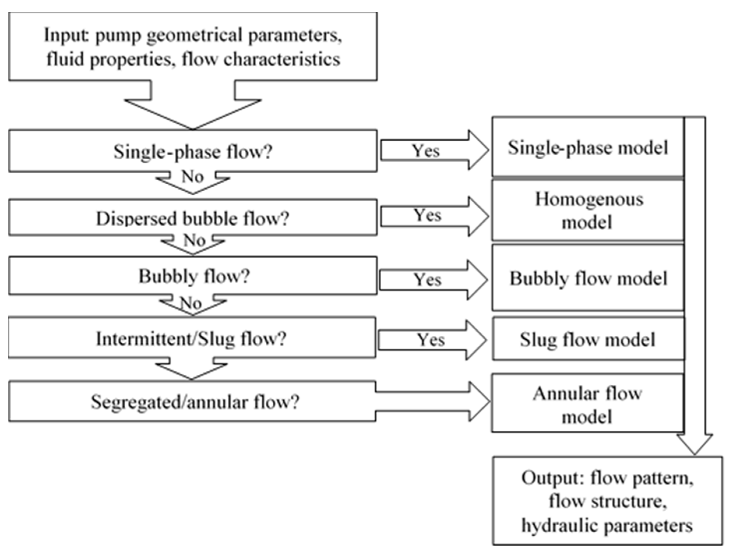
4.4.3. Mechanistic Model Calculation

For the mechanistic models of two-phase flow in a rotating ESP discussed above, a calculation flow chart is given below in Figure 19.
From our previous studies [1,90,122], the inputs of the mechanistic model contain pump geometrical parameters such as radius, blade angles, channel volume and cross sectional area etc., as well as the fluid properties, e.g., gas/liquid density, viscosities, surface tension. The ESP operation conditions (rotational speed, flow rates etc.) are also required. The flow pattern transition boundaries are similar to two-phase pipe flow. The flow map can be divided into four different flow regimes, namely dispersed bubble flow, bubbly flow, intermittent flow, and segregated flow. Based on the limited visualization results, the intermittent and segregated flows in a rotating ESP are slug flow and co-current annular flow, respectively.
With the flow pattern determined, the respective flow model can be called to solve the governing equations to obtain the flow structure and other hydraulic parameters, among which the in-situ gas void fraction (αG) inside the rotating impeller is the most important parameter to estimate ESP boosting pressure under gassy flow conditions.

5. Closure Relationship
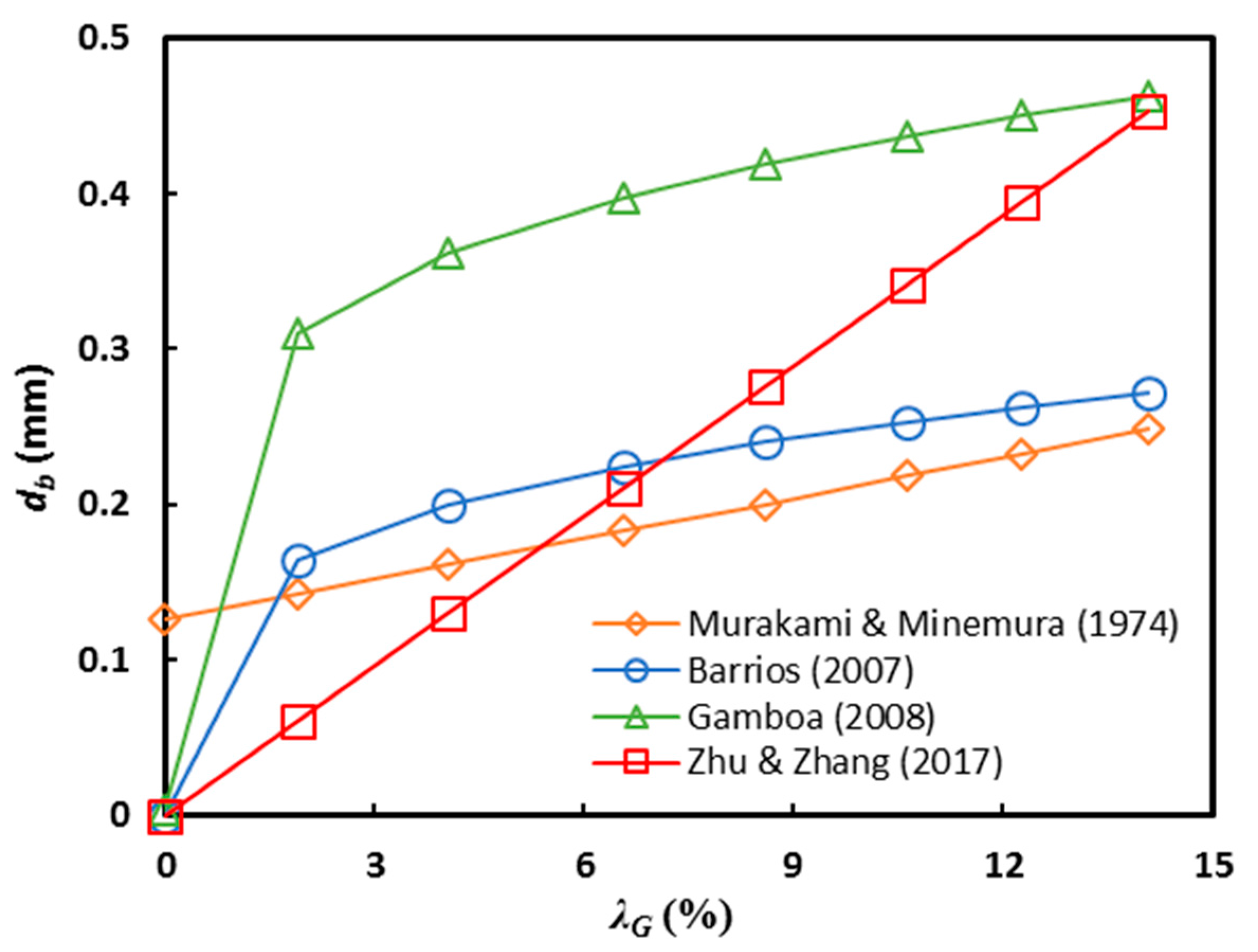
In mechanistic or numerical models, the closure relationships are needed on top of the conservation equations. The closure relationships in modeling centrifugal pump two-phase performance include bubble size, drag force coefficient, in-situ gas void fractions, friction factors etc.

5.1. Bubble Size

The bubble size prediction is a critical closure relationship in mechanistic modeling of ESP performance under gassy conditions. However, a generally validated mechanistic model for predicting bubble size in centrifugal pumps is not available. Several proposed bubble size models for centrifugal pump are either empirical or semi-empirical. They were verified with specific pumps and air/water as working fluids [31,32,39,40]. The generality of these models is questionable. The bubble characteristics inside the rotating impeller are affected by many factors, including fluid properties (density, viscosity, surface tension), pump geometry and operating parameters (rotational speed, flow rates).
By photographing the bubble dispersion in a pump with a transparent Plexiglas casing, Murakami and Minemura [31,32] correlated the observed bubble sizes with a linear relationship of Sauter Mean Diameter (d32) versus GVF (Equation (29)):
d m = 21.82 ( N 6.862 ) 3 4 ( 0.618 + 4.273 λ )
Although Equation (27) is based on rotational speed (N) and inlet GVF, the empirical nature limited its applicability (λ < 8%, 1000 < N < 1500 rpm). Another model of bubble size in a centrifugal pump was proposed by Estevam [64] based on analogy to gas-liquid two-phase pipe flow. Applying Hinze [123] theory for droplet breakup mechanism in turbulent flow to bubble size prediction in centrifugal pump, Estevam obtained the following equation to calculate the maximum dispersed bubble size:
d max = 1.17 ( σ ρ l ) 3 5 ( 2 f β , ω D H ) 2 5
where the constant of 1.17 is a parameter accounting for the curvature of impeller flow passages; σ, ρl and DH are interfacial tension, liquid density and hydraulic diameter, respectively; the friction factor (fβ,ω) is determined by analogy to fluid flow in pipeline and considering rotational speed effect.
Following a similar methodology of modeling bubble size inside a centrifugal pump, Barrios [39] proposed a bubble size prediction model based on the visualization experimental data inside ESP taken by high-speed camera. Barrios pointed out that the experimental results were necessary to determine the relationship of the maximum bubble size, the critical bubble size and inlet GVF. The critical Weber number (Wecrit) is a parameter dominating gas bubble breakup. Hence, Equation (30) explicitly relates the bubble size with the rotational speed and liquid properties:
d b _ s u r g = 0.0348 N 0.8809 λ 1 / 4 ( σ ρ l ) 3 / 5 1 ( N 3 r 1 2 ) 2 / 5
where r1 is the impeller radius. Gamboa [40] employed the Levich [124] model for maximum stable bubble size in pipe flow and proposed an alternative way of modeling bubble size inside an ESP. Gamboa improved the bubble size model by introducing dispersed gas phase density and Wecrit based on Kouba [125] droplet breakup studies:
d max = 14.27 ( σ ρ l ) 3 / 5 ( ( Ω D ) 4 ν ) 2 / 5 ( ρ l ρ g ) 1 / 5 ( 1 + 191.7 λ 0.2 )
where ρg is in-situ gas density, v is liquid kinetic viscosity and Ω, D are impeller rotational speed and diameter, respectively.
A new correlation for computing the representative bubble sizes inside or rotating ESP impeller was recently proposed by Zhu and Zhang [105], as given by Equation (31). The model is based on CFD simulations of pump pressure increment under gassy flows, where the bubble size plays a dominant role to make the numerically simulated ESP heads comparable to the corresponding experimental data. The proposed correlation was verified by further comparisons of the CFD simulation results with the incorporation of Equation (33) against the experimental pump pressure increment, which shows a good match:
d 32 = 6.034 λ G ( σ ρ c ) 3 / 5 ( Δ P q ρ c V ) 2 / 5 ( ρ c ρ d ) 1 / 5
where d32 is the Sauter mean diameter; λG is the inlet gas volumetric fraction; subscripts of c and d denote continuous and dispersed phases, respectively. ΔP is the pressure increment of ESP under single-phase flow; V is the volume of the entire impeller flow domain.
The comparison of existing bubble size models in literature is shown in Figure 20, where the horizontal axis corresponds to λG and the vertical axis shows the calculated bubble diameters. As can be seen, the predicted bubble sizes in the rotating ESP impeller by different models vary significantly. The reason might be due to the derivation of prediction model that is based on either empirical constant or partial regression of experimental data. The complex physical reality of multiphase flow through a rotating ESP impeller further contributes to the difficulty of reaching a generally validated prediction model of bubble size. Meanwhile, the mutual validation among different models seems to be unavailable due to the lack of relevant experimental measurement of in-situ bubble sizes as well as geometrical details (channel volume etc.). A similar trend of db versus λG is used by Barrios [39] and Gamboa [40] to correlate the experimental measurement of bubble diameters. However, the linear relationship of db versus λG is applied by Murakami and Minemura [31,32], and Zhu and Zhang [105] studies, where a good agreement between the model predicted db against either visualization experiments or CFD simulation results can be reached.
Although several models are available in literature for bubble size prediction in a centrifugal pump with rotating turbulent flow, their empirical/semi-empirical natures limited the range of applications. As discussed by Gamboa [40], the challenge in modeling bubble size inside a rotating ESP is the mechanism that dominates bubble formation, including coalescence and breakup. Therefore, investigation is needed to better understand the bubble dispersion mechanism and develop better model for bubble size prediction.

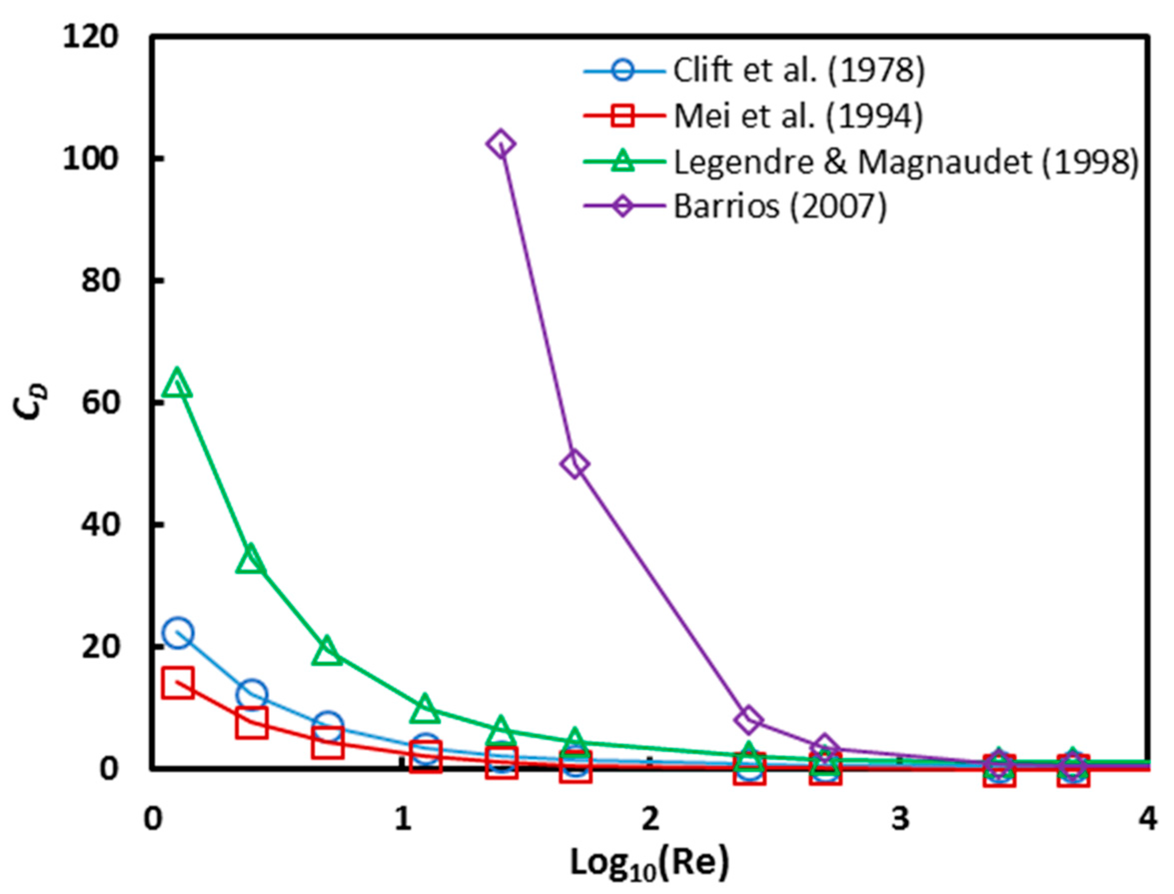
5.2. Drag Coefficient

In gas-liquid two-phase flow, the drag force is the interfacial momentum transfer due to velocity difference between gas and liquid phases [102]:
F D = C D A p ρ f ( U v ) | U v | 2
where U and v are velocities of liquid and gas phases, respectively. The drag coefficient (CD) for bubbles in no-rotating flow fields without shearing was studied by Schiller and Naumann [126], Clift et al. [127], Ishii and Zuber [128], Mei et al. [129] among others. Schiller and Naumann proposed an empirical correlation of CD for 0.1 < Re < 800. Clift et al. developed a more accurate expression which is valid for higher Re up to 3 × 10⁵ [130]:
C D = 24 Re ( 1 + 0.15 Re 0.687 ) + 0.42 1 + 4.25 × 10 4 Re 1.16
Ishii and Zuber incorporated a correlation term (1 + αd)γ to account for effects of bubble volumetric fraction and flow regime, where γ is an empirical constant determined by fluid properties and particle shapes. Mei et al. [129] studied the behavior of clean bubbles (no contaminations or surfactants involved) in a uniform flow and proposed an empirical drag CD for 0.1 < Re < 100:
C D = 16 Re ( 1 + ( 8 Re + 1 2 ( 1 + 3.315 Re 1 2 ) ) 1 )
For shear-induced flow, the viscous drag force exerted on bubbles is increased by broadening the near wake [131]. Thus, the dimensionless shear rate, Strouhal number (Sr) as an indicator of shear strength, was employed by Legendre and Magnaudet [132] to calculate CD in shear flow for moderate-to-large Re (≥50):
S r = d b ω | U v |
and:
C D , s r = C D , 0 ( 1 + 0.55 S r 2 )
where CD,0 is the drag coefficient calculated without shear effect [131]. Rastello et al. [133,134] revised Equation (36) to get a better fitting of their experimental data for low, moderate and high Reynolds numbers with a broad range of Sr:
C D , s r = C D , 0 ( 1 + 0.3 S r 2.5 )
Barrios [39] measured bubble sizes inside a single-stage ESP with a visualization experimental system and calculated the drag coefficients on stagnant bubbles in rotating flow field. Then, the drag coefficients were correlated by:
C D = 24 Re Y ( 1 + f ( Re , Y ) )
where Y and f (Re,Y) are given by:
f ( Re , Y ) = 5.48 24 ( Re Y ) 0.427 + 0.36 24 ( Re Y )
and:
Y = 0.00983 + 389.9 Re N 2
Figure 21 shows the comparison of drag coefficients predicted by the empirical models discussed above. As can be seen, the evident discrepancy is observed under relatively low Reynolds number with/without considering the rotating effects in flow fields. At higher Reynolds number, the similar drag coefficients, which are close to 0.44, can be obtained from the existing empirical models. The drag coefficients predicted by Clift et al. [127] and Mei et al. [128] is close to each other due to neglecting rotation flow. However, when accounting for fluid rotating effect, the model predictions of CD vary significantly. Barrios [39] correlation outputs CD that is several times larger than that calculated by Legendre and Magnaudet [132] model. A possible explanation is that Barrios model is specifically on basis of the bubble flow inside a rotating ESP impeller, while the Legendre and Magnaudet model is regressed from a single bubble flowing inside a rotating cylinder.

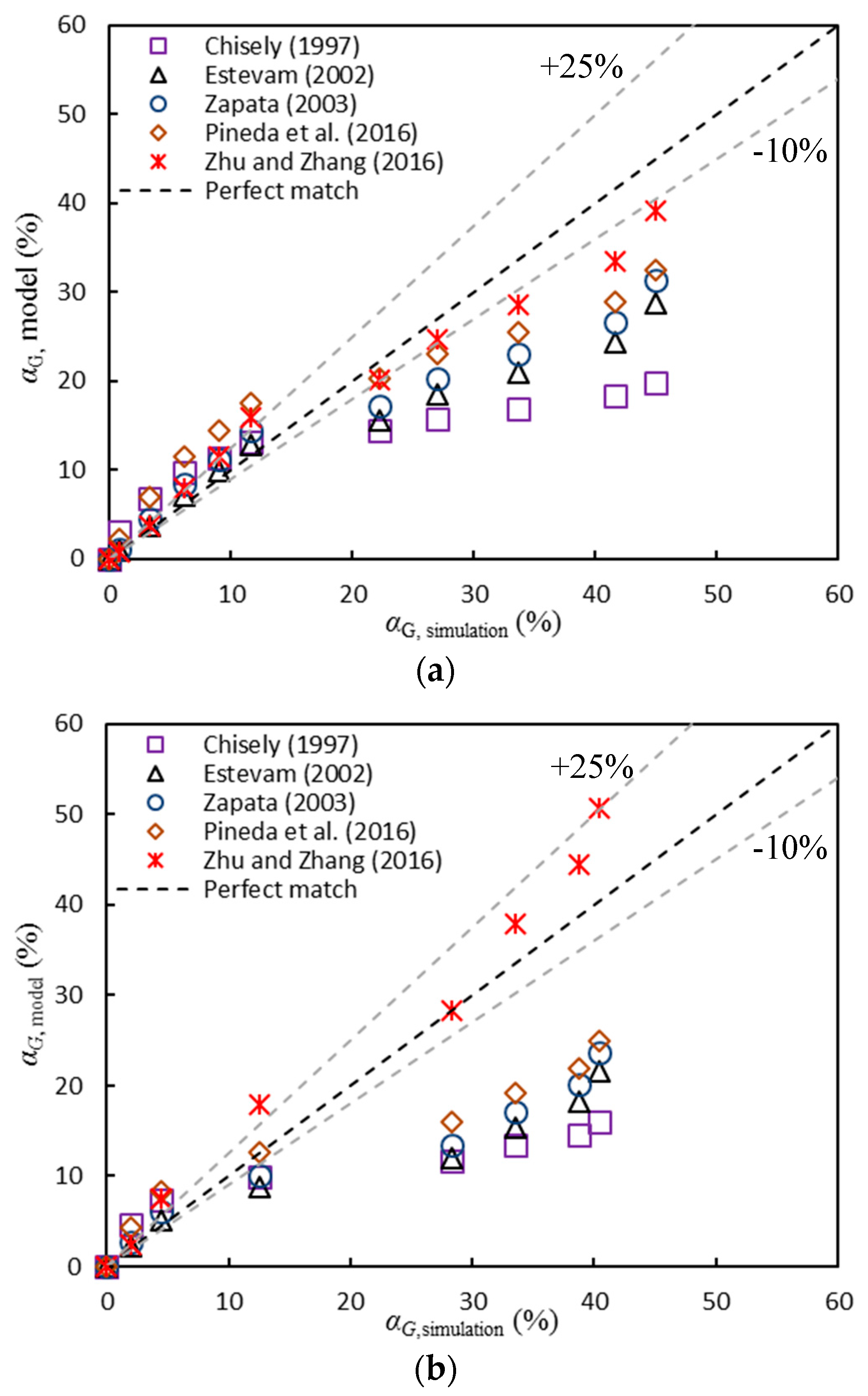
5.3. In-Situ Gas Void Fraction (αG)

The in-situ gas void fraction (αG) is an important variable in two-phase flow related to the velocity slippage between two immiscible phases and the gas accumulation. Moreover, αG is needed to determine the in-situ gas/liquid mixture density by ρ M = α G ρ G + ( 1 α G ) ρ L , which in turn affects the pump boosting pressure significantly according to P M = ρ M g H M . ρM is the mixture density, and HM is the hydraulic head of ESP with gas/liquid flow. However, due to the complicated pump geometries and fluid flow dynamics in the ESP impeller, it is challenging to develop a mechanistic model to predict αG with general validity. Very few studies on mechanistic modeling of local gas void fraction in ESPs can be found in literature so far.
The simplest model for predicting αG in multiphase centrifugal pump flows is the homogeneous model, which assumes no slippage between gas and liquid phases:
α G = λ G = Q G Q G + Q L
The homogenous model is valid for very low inlet GVFs when the slippage between gas and liquid is minimal. Errors will result from applying the homogeneous model to flow conditions with high inlet GVFs when the slippage is not negligible. Accounting for the phase slippage, several empirical correlations were proposed by Chisely [62], Estevam [64], Zapata [38] and Pineda et al. [114], among others.
Chisely studied loss of coolant accident with a volute-type centrifugal pump in the nuclear industry. The pressure distribution and flow regimes were determined with the experimental measurement and high-speed photographing. A model for predicting the centrifugal pump pressure increment under two-phase flow conditions was proposed. To make this model solvable, the in-situ αG was correlated as:
α G = [ 1 + 0.28 ( 1 x x ) 0.64 ( ρ G ρ L ) 0.36 ( μ L μ G ) 0.07 ] 1
where χ is the gas quality, μG and μL are the gas and liquid viscosities.
Zapata experimentally studied the rotational speed effect on ESP two-phase performance. Using least-square regression, a new correlation of αG was presented to predict the pump boosting pressure. The empirical correlation as function of gas and liquid flow rates and the rotational speed is given as:
α G = [ ( q G q max ) ( q L / q max ) 1.277 0.034 N d N d 0.598 + 0.223 N d N d ] 1 0.921 + 0.068 N d N d
where qG and qL are the gas and liquid flow rates, N d N d is normalized rotational speed, and qmax is the maximum single-phase liquid flow rate.
Pineda et al. [114] proposed an empirical correlation based on the Lockhart-Martinelli type parameter Xtt by non-linear regression of CFD simulated values of in-situ αG:
α G = 7.119 X t t 0.8778 0.002138
where:
X t t = ( μ L μ G ) 0.1 ( 1 x x ) 0.9 ( ρ G ρ L ) 0.5
Zhu and Zhang [90] proposed a mechanistic model to compute the in-situ gas void fraction. The model prediction was validated by the 3D CFD simulation. A better match over the existing empirical models was achieved. The model is based on the balance of centrifugal buoyancy force and drag force on a stable gas bubble in ESP, which incorporates the gas-liquid interaction mechanism and is applicable to a wide flow conditions. The prediction model is given as,
α G = R S 1 + ( 1 R S ) 2 + 4 R S λ G 2 R S
where:
R S = V S R ( 2 π R I Z I T B ) Y I Q + Q L K
VSR is the slippage velocity in radial direction, RI is the representative impeller radius, ZI is the impeller number, TB is the blade thickness, YI is the impeller channel height, Q and QLK is the liquid flow rate and its corresponding leakage flow rate. The drag coefficient is calculated by
C D = { C D , 0 ( 1 + 0.55 S r 2 ) Re > 50 C D , 0 ( 1 + 0.3 S r 2.5 ) Re 50
where Sr is Strouhal number and defined by S r = d B Ω / | U v | . U and v are phase velocities. CD,0 is the drag coefficient proposed by Clift et al. [127] without consideration of shear effect.
Figure 22 shows the comparison of existing models in predicting in-situ gas void fraction in a rotating pump impeller. As can be seen, Zhu and Zhang [90] model predicts in-situ αG with an error less than 25%, and most predictions are bounded by 10% error line. Nevertheless, αG predicted by previous empirical correlations deviates from CFD simulated αG increasingly as inlet λG increases. Since most of the correlations were based on homogeneous assumption rather than velocity slippage between gas and liquid phases, the predictions from empirical correlations are acceptable only at low λG. For relatively higher λG, the phase slippage dominates bubble behaviors, which results in the failure of empirical correlations.

6. Conclusions and Future Work

In this paper, the experimental studies and modeling approaches for investigating gas/liquid two-phase flow inside a rotating electrical submersible pump have been reviewed in detail. Different empirical and mechanistic models for predicting ESP boosting pressure under gassy flows were discussed. The state-of-art CFD-based numerical simulation as a complemental method for ESP two-phase performance prediction was elaborated.
The review of the published experimental studies for gas-liquid flow in centrifugal pumps has highlighted the complications behind the accurate prediction of two-phase performance inside a rotating ESP. The turbulent flow with transient behaviors make it difficult to visualize the internal flow structures and flow patterns. This is not helped by the twisted blade/vane geometries and multistage assembly. Due to these observation difficulties, the multiphase flow mechanisms that dominate the ESP head degradation were not well understood. This in turn delayed the development of mechanistic models. Although CFD simulation serves as an alternative way to study multiphase flow, its validity and reliability, especially coupled with the strong shearing effect and phase interactions are questioned.
The ESP performance under gassy flow is affected by many factors. There is room for further improvements on the mechanistic modeling and prediction:
  • Experimental visualization of internal two-phase flow structures in a rotating ESP is inadequate, which restricts the flow pattern assessment and the formulations of governing equations. Moreover, the measurement of in-situ gas phase is insufficient, resulting in further difficulty to characterize pump performance quantitatively. Future experimental work should take these challenges into consideration, thus providing in-depth knowledge of multiphase flow mechanisms in ESPs.
  • The computational fluid dynamics techniques need to be further developed in order to capture the complex behaviors and movement of gas bubbles inside ESPs and thus better understand the interactions between the gas and liquid phases in different flow patterns.
  • The mechanistic models should focus more on the physics of the two-phase flow in rotating ESPs to propose better closure relationships. From the one-dimensional two-fluid model, the simplified mass and momentum conservation equations are solvable with the help of the improved closure relationships in future, ending up with a more accurate and reliable mechanistic model to predict ESP two-phase flow performance.

Acknowledgments

The authors appreciate the technical and financial support of the Tulsa University Artificial Lift Projects (TUALP) member companies. The work is supported by the National Natural Science Foundation-Outstanding Youth Foundation (51622405).

Conflicts of Interest

The authors declare no conflict of interest.

Nomenclature

Aarea, L2, m2
achannel length, L, m
bblade thickness, L, m; or channel width, L, m
BEPbest efficiency point
BHPbrake horsepower, ML2/T3, kg∙m2/s3
Cabsolute velocity, L/T, m/s
CDdrag coefficient
Cmdisk friction coefficient
Cpdiffuser loss coefficient
dbubble diameter, L, m
D1tdiameter at tip of inlet, L, m
Dfdiffusion factor
DHhydraulic diameter, L, m
Diimpeller diameter, L, m
ffriction factor
fdiskdisk friction loss coefficient
fEliquid entrainment factor
fgeoshape factor dependent on the impeller diameters and the angle between the sidewall of the rotor and the pump shaft
F interfacial force vector, M/(LT2), Pa
g gravity acceleration vector, L/(T2), m/s2
GVFgas volumetric fraction
hchannel height, L, m or hydraulic head, L, m
Hhydraulic head, L, m or holdup
kturbulent kinetic energy, L2/(T2), m2/s2
kRRfriction factor
m ˙ mass flow rate, M/T, kg/s
Mmomentum transfer term per unit volume, M/(L2T2), Pa/m
nphase number
Nrotational speed, 1/L, rpm
ppressure, M/(LT2), Pa
ΔPstage pressure increment, M/(LT2), Pa
Ppressure, M/(LT2), Pa
qflow rate, L3/T, m3/s
Qmass flow rate, M/T, kg/s
rradius, L, m
rHhydraulic radius, L, m
ReReynolds number
sstreamline, L, m
SrStrouhal number
ttime, T, s
Ttorque, (ML2)/T2, kg∙m2/s2
u i phase velocity vector, L/T, m/s
Uperipheral velocity, L/T, m/s
vvelocity, L/T, m/s
vvelocity fluctuation, L/T, m/s
Vvelocity, L/T, m/s
Volvolume, L3, m3
Wrelative velocity in ESP, L/T, m/s
WeWeber number
xmass fraction or mole fraction
Ychannel height, L, m
Zblade number
Greek Symbols
αgas void fraction, or absolute flow angle formed between the absolute
velocity and its tangential component
βtangential blade angle, deg
λGno-slip gas void fraction (GVF)
μdynamic viscosity, M/(LT), Pa∙s
μtturbulent viscosity, M/(LT), Pa∙s
Ωangular speed, 1/T, rad/s
ωshaft or impeller blades angular velocity, 1/T, rad/s
ρfluid density, M/L3, kg/m3
σsurface tension, M/T2, N/m or slip factor
τ ¯ ¯ stress-strain tensor, M/(LT2), Pa
εturbulent energy dissipation rate per unit mass, L2/T3, m2/s3
θcomponent of the radial coordinate system
Subscripts
1inlet
2outlet
32Sauter mean diameter
Bbubble or blade
b_surgbubble at pressure surging
ccontinuous phase
Cgas core or critical
CRITcritical
ddiffuser or dispersed phase or dimensionless parameter
Ddiffuser
effeffective
EEuler
Ffilm
FIfluid in ESP impeller
FDfluid in ESP diffuser
Ggas phase
Hhydraulic parameter
Iinterface or impeller
Lliquid phase
LFliquid film
Mmeridional direction or mixture
mmixture
Rradius direction
spheresphere
streamline projection on streamline
Sspecific speed or shear or slug body
SGsuperficial gas
SIimpeller channel wall
SLsuperficial liquid
SRshear in the radial direction
Uperipheral direction
vmvirtual mass
wwater
Wwall
Units
bpdbarrel per day, 1 bpd ≈ 1.8942 × 10⁻⁶ m3/s
psipound per square inch, 1 psi ≈ 6894.76 pa
psiapound per square inch for absolute pressure
psigpound per square inch for gauge pressure

References

  1. Zhu, J. Experiments, CFD Simulation and Modeling of ESP Performance under Gassy Conditions. Ph.D. Thesis, The University of Tulsa, Tulsa, OK, USA, 2017. [Google Scholar]
  2. Barrios, L.; Rojas, M.; Monteiro, G.; Sleight, N. Brazil field experience of ESP performance with viscous emulsions and high gas using multi-vane pump MVP and high power ESPs. In Proceedings of the SPE Electric Submersible Pump Symposium, The Woodlands, TX, USA, 24–28 April 2017. [Google Scholar]
  3. Takacs, G. Electrical Submersible Pumps Manual: Design, Operations, and Maintenance; Gulf Professional Publishing: Burlington, NY, USA, 2009. [Google Scholar]
  4. Oliva, G.B.; Galvão, H.L.; dos Santos, D.P.; Silva, R.E.; Maitelli, A.L.; Costa, R.O.; Maitelli, C.W. Gas effect in electrical-submersible-pump-system stage-by-stage analysis. SPE Prod. Oper. 2017, 32, 294–304. [Google Scholar] [CrossRef]
  5. Zhou, D.; Sachdeva, R. Simple model of electric submersible pump in gassy well. J. Pet. Sci. Eng. 2010, 70, 204–213. [Google Scholar] [CrossRef]
  6. Stepanoff, A.J. Centrifugal and Axial Flow Pumps: Theory, Design and Application, 2nd ed.; John Wiley & Sons: New York, NY, USA, 1957. [Google Scholar]
  7. Vieira, T.S.; Siqueira, J.R.; Bueno, A.D.; Morales, R.E.M.; Estevam, V. Analytical study of pressure losses and fluid viscosity effects on pump performance during monophase flow inside an ESP stage. J. Pet. Sci. Eng. 2015, 127, 245–258. [Google Scholar] [CrossRef]
  8. Ito, H. Friction factors for turbulent flow in curved pipes. J. Basic Eng. 1959, 81, 123–134. [Google Scholar]
  9. Jones, O.C. An improvement in the calculation of turbulent friction in rectangular ducts. J. Fluids Eng. 1976, 98, 173–180. [Google Scholar] [CrossRef]
  10. Churchill, S.W. Friction-factor equation spans all fluid-flow regimes. Chem. Eng. 1977, 84, 91–92. [Google Scholar]
  11. Shah, R.K. A correlation for laminar hydrodynamic entry length solutions for circular and noncircular ducts. J. Fluids Eng. 1978, 100, 177–179. [Google Scholar] [CrossRef]
  12. Sun, D. Modeling Gas-Liquid Head Performance of Electrical Submersible Pumps. Ph.D. Thesis, The University of Tulsa, Tulsa, OK, USA, 2003. [Google Scholar]
  13. Wiesner, F.J. A review of slip factors for centrifugal impellers. J. Eng. Power 1967, 89, 558–566. [Google Scholar] [CrossRef]
  14. Sun, D.; Prado, M.G. Single-phase model for electric submersible pump (ESP) head performance. SPE J. 2006, 11, 80–88. [Google Scholar] [CrossRef]
  15. Thin, K.C.; Khaing, M.M.; Aye, K.M. Design and performance analysis of centrifugal pump. World Acad. Sci. Eng. Technol. 2008, 46, 422–429. [Google Scholar]
  16. Ito, H.; Nanbu, K. Flow in rotating straight pipes of circular cross section. J. Basic Eng. 1971, 93, 383–394. [Google Scholar] [CrossRef]
  17. Bing, H.; Tan, L.; Cao, S.; Lu, L. Prediction method of impeller performance and analysis of loss mechanism for mixed-flow pump. Sci. China Technol. Sci. 2012, 55, 1988–1998. [Google Scholar] [CrossRef]
  18. Amaral, G. Single-Phase Flow Modeling of an ESP Operating with Viscous Fluids. Master’s Thesis, State University of Campinas, Campinas, São Paulo, Brazil, 2007. [Google Scholar]
  19. Gülich, J.F. Pumping highly viscous fluids with centrifugal pumps—Part 1. World Pumps 1999, 395, 30–34. [Google Scholar] [CrossRef]
  20. Gülich, J.F. Pumping highly viscous fluids with centrifugal pumps—Part 2. World Pumps 1999, 396, 39–42. [Google Scholar] [CrossRef]
  21. Tuzson, J. Centrifugal Pump Design; John Wiley & Sons: New York, NY, USA, 2000. [Google Scholar]
  22. Sun, D.; Prado, M.G. Modeling gas-liquid head performance of electric submersible pumps. J. Press. Vessel Technol. 2005, 127, 31–38. [Google Scholar] [CrossRef]
  23. Van Esch, B.P.M. Simulation of Three-Dimensional Unsteady Flow in Hydraulic Pumps. Master’s Thesis, University of Twente, Enschede, The Netherlands, 1997. [Google Scholar]
  24. Ladouani, A.; Nemdili, A. Influence of Reynolds number on net positive suction head of centrifugal pumps in relation to disc friction losses. Forsch. Ing. 2009, 73, 173. [Google Scholar] [CrossRef]
  25. Ippen, A.T. The Influence of Viscosity on Centrifugal Pump Performance; Issue 199 of Fritz Engineering Laboratory Report, ASME Paper No. A-45-57; The American Society of Mechanical Engineers: New York, NY, USA, 1945. [Google Scholar]
  26. Li, W.G. Experimental investigation of performance of commercial centrifugal oil pump. World Pumps 2002, 425, 26–28. [Google Scholar] [CrossRef]
  27. Amaral, G.; Estevam, V.; França, F.A. On the influence of viscosity on ESP performance. SPE Prod. Oper. 2009, 24, 303–310. [Google Scholar] [CrossRef]
  28. Solano, E.A. Viscous Effects on the Performance of Electro Submersible Pumps (ESP’s). Master’s Thesis, The University of Tulsa, Tulsa, OK, USA, 2009. [Google Scholar]
  29. Barrios, L.J.; Scott, S.L.; Sheth, K.K. ESP technology maturation: Subsea boosting system with high GOR and viscous fluid. In Proceedings of the SPE Annual Technical Conference and Exhibition, San Antonio, TX, USA, 8–10 October 2012. [Google Scholar]
  30. Banjar, H.M.; Gamboa, J.; Zhang, H.-Q. Experimental study of liquid viscosity effect on two-phase stage performance of electrical submersible pumps. In Proceedings of the SPE Annual Technical Conference and Exhibition, New Orleans, LA, USA, 30 September–2 October 2013. [Google Scholar]
  31. Murakami, M.; Minemura, K. Effects of entrained air on the performance of a centrifugal pump (1st report, performance and flow conditions). Bull. JSME 1974, 17, 1047–1055. [Google Scholar] [CrossRef]
  32. Murakami, M.; Minemura, K. Effects of entrained air on the performance of a centrifugal pump (2nd report, effects of number of blades). Bull. JSME 1974, 17, 1286–1295. [Google Scholar] [CrossRef]
  33. Cirilo, R. Air-Water Flow through Electric Submersible Pumps. Master’s Thesis, The University of Tulsa, Tulsa, OK, USA, 1998. [Google Scholar]
  34. Romero, M. An Evaluation of an Electric Submersible Pumping System for High GOR Wells. Master’s Thesis, University of Tulsa, Tulsa, OK, USA, 1999. [Google Scholar]
  35. Pessoa, R. Experimental Investigation of Two-Phase Flow Performance of Electrical Submersible Pump Stages. Master’s Thesis, The University of Tulsa, Tulsa, OK, USA, 2001. [Google Scholar]
  36. Beltur, R. Experimental Investigation of Two-Phase Flow Performance of ESP Stages. Master’s Thesis, The University of Tulsa, Tulsa, OK, USA, 2003. [Google Scholar]
  37. Duran, J. Pressure Effects on ESP Stages’ Air-Water Performance. Master’s Thesis, The University of Tulsa, Tulsa, OK, USA, 2003. [Google Scholar]
  38. Zapata, L. Rotational Speed Effects on ESP Two-Phase Performance. Master’s Thesis, The University of Tulsa, Tulsa, OK, USA, 2003. [Google Scholar]
  39. Barrios, L. Visualization and Modeling of Multiphase Performance inside an Electrical Submersible Pump. Ph.D. Thesis, The University of Tulsa, Tulsa, OK, USA, 2007. [Google Scholar]
  40. Gamboa, J. Prediction of the Transition in Two-Phase Performance of an Electrical Submersible Pump. Ph.D. Thesis, The University of Tulsa, Tulsa, OK, USA, 2008. [Google Scholar]
  41. Trevisan, F.E. Modeling and Visualization of Air and Viscous Liquid in Electrical Submersible Pump. Ph.D. Thesis, The University of Tulsa, Tulsa, OK, USA, 2009. [Google Scholar]
  42. Salehi, E. ESP Performance in Two-Phase Flow through Mapping and Surging Tests at Various Rotational Speeds and Intake Pressures. Master’s Thesis, The University of Tulsa, Tulsa, OK, USA, 2012. [Google Scholar]
  43. Croce Mundo, D.D. Study of Water/Oil Flow and Emulsion Formation in Electrical Submersible Pumps. Master’s Thesis, The University of Tulsa, Tulsa, OK, USA, 2014. [Google Scholar]
  44. Zhu, J.; Zhu, H.; Zhang, J.; Zhang, H.-Q. An experimental study of surfactant effect on gas tolerance in electrical submersible pump (ESP). In Proceedings of the ASME 2017 International Mechanical Engineering Congress and Exposition, Tampa, FL, USA, 3–9 November 2017. [Google Scholar]
  45. DeGennes, P.-G.; Brochard-Wyart, F.; Quere, D. Capillarity and Wetting Phenomena; Springer: New York, NY, USA, 2004. [Google Scholar]
  46. Hu, B.; Nienow, A.W.; Stitt, E.H.; Pacek, A.W. Bubble sizes in agitated solvent/reactant mixtures used in heterogeneous catalytic hydrogenation of 2-butyne-1,4-diol. Chem. Eng. Sci. 2006, 61, 6765–6774. [Google Scholar] [CrossRef]
  47. Omer, A.; Pal, R. Effects of surfactant and water concentrations on pipeline flow of emulsions. Ind. Eng. Chem. Res. 2013, 52, 9099–9105. [Google Scholar] [CrossRef]
  48. Van Nimwegen, A.T.; Portela, L.M.; Henkes, R.A. The effect of surfactants on vertical air/water flow for prevention of liquid loading. SPE J. 2015, 4, 488–500. [Google Scholar]
  49. Van Nimwegen, A.T.; Portela, L.M.; Henkes, R.A.W.M. The effect of surfactants on upward air-water pipe flow at various inclinations. Int. J. Multiph. Flow 2016, 78, 132–147. [Google Scholar] [CrossRef]
  50. Ajani, A.; Kelkar, M.; Sarica, C.; Pereyra, E. Effect of surfactants on liquid loading in vertical wells. Int. J. Multiph. Flow. 2016, 83, 183–201. [Google Scholar] [CrossRef]
  51. Ajani, A.; Kelkar, M.; Sarica, C.; Pereyra, E. Foam flow in vertical gas wells under liquid loading: Critical velocity and pressure drop prediction. Int. J. Multiph. Flow 2016, 87, 124–135. [Google Scholar] [CrossRef]
  52. Shoham, O. Mechanistic Modeling of Gas-Liquid Two-Phase Flow in Pipes; Society of Petroleum Engineers: Richardson, TX, USA, 2006. [Google Scholar]
  53. Parsi, M.; Najmi, K.; Najafifard, F.; Hassani, S.; McLaury, B.S.; Shirazi, S.A. A comprehensive review of solid particle erosion modeling for oil and gas wells and pipelines applications. J. Nat. Gas Sci. Eng. 2014, 21, 850–873. [Google Scholar] [CrossRef]
  54. Wu, B.; Firouzi, M.; Mitchell, T.; Rufford, T.E.; Leonardi, C.; Towler, B. A critical review of flow maps for gas-liquid flows in vertical pipes and annuli. Chem. Eng. J. 2017, 326, 350–377. [Google Scholar] [CrossRef]
  55. Taitel, Y.; Bornea, D.; Dukler, A.E. Modelling flow pattern transitions for steady upward gas-liquid flow in vertical tubes. AIChE J. 1980, 26, 345–354. [Google Scholar] [CrossRef]
  56. Minumura, K.; Murakami, M. A theoretical study on air bubble motion in a centrifugal pump impeller. J. Fluids Eng. 1980, 102, 446–455. [Google Scholar] [CrossRef]
  57. Patel, B.R. Investigations into the two-phase flow behavior of centrifugal pumps. In Polyphase Flow in Turbomachinery, Proceedings of the ASME Winter Annual Meeting of the American Society of Mechanical Engineering, San Francisco, CA, USA, 10–15 December 1978; The American Society of Mechanical Engineers: New York, NY, USA; pp. 79–100.
  58. Sekoguchi, K.; Takada, S.; Kanemori, Y. Study of air-water two-phase centrifugal pump by means of electric resistivity probe technique for void fraction measurement: 1st report, measurement of void fraction distribution in a radial flow impeller. Bull. JSME 1984, 27, 931–938. [Google Scholar] [CrossRef]
  59. Kim, J.H.; Duffey, R.B.; Belloni, P. On centrifugal pump head degradation in two-phase flow. In Design Methods for Two-Phase Flow in Turbomachinery; The American Society of Mechanical Engineers: New York, NY, USA, 1985. [Google Scholar]
  60. Sato, S.; Furukawa, A.; Takamatsu, Y. Air-water two-phase flow performance of centrifugal pump impellers with various blade angles. JSME Int. J. Ser. B Fluids Therm. Eng. 1996, 39, 223–229. [Google Scholar] [CrossRef]
  61. Takemura, T.; Kato, H.; Kanno, H.; Okamoto, H.; Aoki, M.; Goto, A.; Egashira, K.; Shoda, S. Development of rotordynamic multiphase pump: The first report. In Proceedings of the International Conference on Offshore Mechanics and Arctic Engineering, Vancouver, BC, Canada, 13–17 April 1997. [Google Scholar]
  62. Chisely, E.A. Two Phase Flow Centrifugal Pump Performance. Ph.D. Thesis, Idaho State University, Pocatello, ID, USA, 1997. [Google Scholar]
  63. Suryawijaya, P.; Kosyna, G. Unsteady measurement of static pressure on the impeller blade surfaces and optical observation on centrifugal pumps under varying liquid/gas two-phase flow condition. J. Comput. Appl. Mech. 2001, 6759, D9–D18. [Google Scholar]
  64. Estevam, V. A Phenomenological Analysis about Centrifugal Pump in Two Phase Flow Operation. Ph.D. Thesis, Universidade Estadual de Campinas, Campinas, Brazil, 2002. [Google Scholar]
  65. Poullikkas, A. Two phase flow performance of nuclear reactor cooling pumps. Prog. Nucl. Energy 2000, 36, 123–130. [Google Scholar] [CrossRef]
  66. Thum, D.; Hellmann, D.H.; Sauer, M. Influence of the patterns of liquid-gas flows on multiphase-pumping of radial centrifugal pumps. In Proceedings of the 5th North American Conference on Multiphase Technology, Banff, AB, Canada, 31 May–2 June 2006. [Google Scholar]
  67. Barrios, L.; Prado, M.G. Experimental visualization of two-phase flow inside an electrical submersible pump stage. J. Energy Resour. Technol. 2011, 133. [Google Scholar] [CrossRef]
  68. Schäfer, T.; Bieberle, A.; Neumann, M.; Hampel, U. Application of gamma-ray computed Tomography for the analysis of gas holdup distributions in centrifugal pumps. Flow Meas. Instrum. 2015, 46, 262–267. [Google Scholar] [CrossRef]
  69. Neumann, M.; Schäfer, T.; Bieberle, A.; Hampel, U. An experimental study on the gas entrainment in horizontally and vertically installed centrifugal pumps. J. Fluids Eng. 2016, 138, 091301. [Google Scholar] [CrossRef]
  70. Verde, W.M.; Biazussi, J.L.; Sassim, N.A.; Bannwart, A.C. Experimental study of gas-liquid two-phase flow patterns within centrifugal pumps impellers. Exp. Therm. Fluid Sci. 2017, 85, 37–51. [Google Scholar] [CrossRef]
  71. Estevam, V.; França, F.A.; Alhanati, F.J. Mapping the performance of centrifugal pumps under two-phase conditions. In Proceedings of the 17th International Congress of Mechanical Engineering, Sao Paulo, Brazil, 10–14 November 2003. [Google Scholar]
  72. Gamboa, J.; Prado, M. Review of electrical-submersible-pump surging correlation and models. SPE Prod. Oper. 2011, 26, 314–324. [Google Scholar] [CrossRef]
  73. Schäfer, T.; Neumann, M.; Bieberle, A.; Hampel, U. Experimental investigations on a common centrifugal pump operating under gas entrainment conditions. Nucl. Eng. Des. 2017, 316, 1–8. [Google Scholar] [CrossRef]
  74. Bieberle, A.; Schlottke, J.; Spies, A.; Schultheiss, G.; Kühnel, W.; Hampel, U. Hydrodynamics analysis in micro-channels of a viscous coupling using gamma-ray computed tomography. Flow Meas. Instrum. 2015, 45, 288–297. [Google Scholar] [CrossRef]
  75. Wagner, M.; Bieberle, A.; Bieberle, M.; Hampel, U. Dynamic bias error correction in gamma-ray computed tomography. Flow Meas. Instrum. 2017, 53, 141–146. [Google Scholar] [CrossRef]
  76. Trevisan, F.; Prado, M. Experimental investigation of the viscous effect on two-phase-flow patterns and hydraulic performance of electrical submersible pumps. J. Can. Pet. Technol. 2011, 50, 45–52. [Google Scholar] [CrossRef]
  77. Paternost, G.M.; Bannwart, A.C.; Estevam, V. Experimental study of a centrifugal pump handling viscous fluid and two-phase flow. SPE Prod. Oper. 2015, 30, 146–155. [Google Scholar] [CrossRef]
  78. Turpin, J.L.; Lea, J.F.; Bearden, J.L. Gas-liquid through centrifugal pumps-correlation of Data. In Proceedings of the Third International Pump Symposium, Houston, TX, USA, 20–22 May 1986. [Google Scholar]
  79. Duran, J.; Prado, M.G. ESP stages air-water two-phase performance—Modeling and experimental data. SPE 120628. Presented at the 2004 SPE ESP Workshop, Houston, TX, USA, 28–30 April 2004. [Google Scholar]
  80. Zakem, S. Determination of gas accumulation and two-phase slip velocity ratio in a rotating impeller. In Polyphase Flow and Transportation Technology, Proceedings of the ASME Century 2 Emerging Technology Conference, San Francisco, CA, USA, 13–15 August 1980; The American Society of Mechanical Engineers: New York, NY, USA; Volume 12, pp. 167–173.
  81. Furuya, O. Analytical model for prediction of two-phase (noncondensable) flow pump performance. J. Fluids Eng. 1985, 107, 139–147. [Google Scholar] [CrossRef]
  82. Sachdeva, R. Two-Phase Flow through Electric Submersible Pumps. Ph.D. Thesis, The University of Tulsa, Tulsa, OK, USA, 1988. [Google Scholar]
  83. Sachdeva, R.; Doty, D.R.; Schmidt, Z. Performance of electric submersible pumps in gassy wells. SPE Prod. Facil. 1994, 2, 55–60. [Google Scholar] [CrossRef]
  84. Minemura, K.; Uchiyama, T.; Shoda, S.; Kazuyuki, E. Prediction of air-water two-phase flow performance of a centrifugal pump based on one-dimensional two-fluid model. J. Fluids Eng. 1998, 120, 327–334. [Google Scholar] [CrossRef]
  85. Gao, C.; Gray, K.E. The development of a coupled geomechanics and reservoir simulator using a staggered grid finite difference approach. In Proceedings of the SPE Annual Technical Conference and Exhibition, San Antonio, TX, USA, 7–12 October 2017. [Google Scholar]
  86. Asuaje, M.; Bakir, F.; Kouidri, S.; Kenyery, F.; Rey, R. Numerical modelization of the flow in centrifugal pump: Volute influence in velocity and pressure fields. Int. J. Rotating Mach. 2005, 3, 244–255. [Google Scholar] [CrossRef]
  87. Maitelli, C.; Bezerra, V.; Da Mata, W. Simulation of flow in a centrifugal pump of ESP systems using computational fluid dynamics. Braz. J. Pet. Gas 2010, 4, 1–9. [Google Scholar]
  88. Rajendran, S.; Purushothaman, K. Analysis of a centrifugal pump impeller using ANSYS-CFX. Int. J. Eng. Res. Technol. 2012, 1, 1–6. [Google Scholar]
  89. Cheah, K.W.; Lee, T.S.; Winoto, S.H.; Zhao, Z.M. Numerical flow simulation in a centrifugal pump at design and off-design conditions. Int. J. Rotating Mach. 2007. [Google Scholar] [CrossRef]
  90. Zhu, J.; Zhang, H.-Q. Mechanistic modeling and numerical simulation of in-situ gas void fraction inside ESP impeller. J. Nat. Gas Sci. Eng. 2016, 36, 144–154. [Google Scholar] [CrossRef]
  91. Gonzalez, J.; Fernandez, J.; Blanco, E.; Santolaria, C. Numerical simulation of the dynamic effects due to impeller-volute interaction in a centrifugal pump. J. Fluids Eng. 2002, 124, 348–355. [Google Scholar] [CrossRef]
  92. Gonzalez, J.; Santolaria, C. Unsteady flow structure and global variables in a centrifugal pump. J. Fluids Eng. 2006, 128, 937–946. [Google Scholar] [CrossRef]
  93. Huang, S.; Mohamad, A.A.; Nandakumar, K.; Ruan, Z.Y.; Sang, D.K. Numerical simulation of unsteady flow in a multistage centrifugal pump using sliding mesh technique. Prog. Comput. Fluid Dyn. 2010, 10, 239–245. [Google Scholar] [CrossRef]
  94. Huang, S.; Su, X.; Guo, J.; Yue, L. Unsteady numerical simulation for gas-liquid two-phase flow in self-priming process of centrifugal pump. Energy Convers. Manag. 2014, 85, 694–700. [Google Scholar] [CrossRef]
  95. Shojaeefard, M.H.; Tahani, M.; Ehghaghi, M.B.; Fallahian, M.A.; Beglari, M. Numerical study of the effects of some geometric characteristics of a centrifugal pump impeller that pumps a viscous fluid. Comput. Fluids 2012, 60, 61–70. [Google Scholar] [CrossRef]
  96. Shojaeefard, M.H.; Boyaghchi, F.A.; Ehghaghi, M.B. Experimental study and three-dimensional numerical flow simulation in a centrifugal pump when handling viscous fluids. IUST Int. J. Eng. Sci. 2006, 17, 53–60. [Google Scholar]
  97. Sirino, T.; Stel, H.; Morales, R.E. Numerical study of the influence of viscosity on the performance of an electrical submersible pump. In Proceedings of the ASME 2013 Fluids Engineering Division Summer Meeting, Incline Village, NV, USA, 7–11 July 2013. [Google Scholar]
  98. Stel, H.; Sirino, T.; Prohmann, P.R.; Ponce, F.; Chiva, S.; Morales, R.E. CFD investigation of the effect of viscosity on a three-stage electric submersible pump. In Proceedings of the ASME 2014 4th Joint US-European Fluids Engineering Division Summer Meeting Collocated with the ASME 2014 12th International Conference on Nanochannels, Microchannels, and Minichannels, Chicago, IL, USA, 3–7 August 2014. [Google Scholar]
  99. Stel, H.; Sirino, T.; Ponce, F.J.; Chiva, S.; Morales, R.E.M. Numerical investigation of the flow in a multistage electric submersible pump. J. Pet. Sci. Eng. 2015, 136, 41–54. [Google Scholar] [CrossRef]
  100. Li, W.G. Mechanism for onset of sudden-rising head effect in centrifugal pump when handling viscous oils. J. Fluids Eng. 2014, 136. [Google Scholar] [CrossRef]
  101. Flores, N.G.; Goncalves, E.; Rolland, J.; Rebattet, C. Head drop of a spatial turbopump inducer. J. Fluids Eng. 2008, 130. [Google Scholar] [CrossRef]
  102. Jeanty, F.; De Andrade, J.; Asuaje, M.; Kenyery, F.; Vásquez, A.; Aguillón, O.; Tremante, A. Numerical simulation of cavitation phenomena in a centrifugal pump. In Proceedings of the ASME 2009 Fluids Engineering Division Summer Meeting, Vail, CO, USA, 2–6 August 2009; pp. 331–338. [Google Scholar]
  103. Barrios, L.; Prado, M.G.; Kenyery, F. CFD modeling inside an electrical submersible pump in two-Phase flow condition. In Proceedings of the ASME 2009 Fluids Engineering Division Summer Meeting, Vail, CO, USA, 2–6 August 2009; Volume 1, pp. 457–469. [Google Scholar]
  104. Zhu, J.; Zhang, H.-Q. CFD simulation of ESP performance and bubble size estimation under gassy conditions. In Proceedings of the SPE Annual Technical Conference and Exhibition, Amsterdam, The Netherlands, 29 October 2014. [Google Scholar]
  105. Zhu, J.; Zhang, H.-Q. Numerical study on electrical-submersible-pump two-phase performance and bubble-size modeling. SPE Prod. Oper. 2017, 32, 267–278. [Google Scholar] [CrossRef]
  106. Minemura, K.; Uchiyama, T. Three-dimensional calculation of air-water two-phase flow in centrifugal pump impeller based on a bubbly flow model. J. Fluids Eng. 1993, 115, 766–771. [Google Scholar] [CrossRef]
  107. Tremante, A.; Moreno, N.; Rey, R.; Noguera, R. Numerical turbulent simulation of the two-phase flow (liquid/gas) through a cascade of an axial pump. J. Fluids Eng. 2002, 124, 371–376. [Google Scholar] [CrossRef]
  108. Caridad, J.; Kenyery, F. CFD analysis of electric submersible pumps (ESP) handling two-phase mixtures. J. Energy Resour. Technol. 2004, 126, 99–104. [Google Scholar] [CrossRef]
  109. Caridad, J.; Asuaje, M.; Kenyery, F.; Tremante, A.; Aguillón, O. Characterization of a centrifugal pump impeller under two-phase flow conditions. J. Pet. Sci. Eng. 2008, 63, 18–22. [Google Scholar] [CrossRef]
  110. Qi, X.; Turnquist, N.; Ghasripoor, F. Advanced electric submersible pump design tool for geothermal applications. GRC Trans. 2012, 36, 543–548. [Google Scholar]
  111. Marsis, E.; Pirouzpanah, S.; Morrison, G. CFD-based design improvement for single-phase and two-phase flows inside an electrical submersible pump. In Proceedings of the ASME 2013 Fluids Engineering Division Summer Meeting, Incline Village, NV, USA, 7–11 July 2013. [Google Scholar]
  112. Yu, Z.; Zhu, B.; Cao, S. Interphase force analysis for air-water bubbly flow in a multiphase rotodynamic pump. Eng. Comput. 2015, 32, 2166–2180. [Google Scholar] [CrossRef]
  113. Yu, Z.Y.; Zhu, B.S.; Cao, S.L.; Wang, G.Y. Application of two-fluid model in the unsteady flow simulation for a multiphase rotodynamic pump. In Proceedings of the IOP Conference Series: Materials Science and Engineering, Kuala Lumpur, Malaysia, 2–4 July 2013; p. 52. [Google Scholar]
  114. Pineda, H.; Biazussi, J.; López, F.; Oliveira, B.; Carvalho, R.D.; Bannwart, A.C.; Ratkovich, N. Phase distribution analysis in an Electrical Submersible Pump (ESP) inlet handling water-air two-phase flow using Computational Fluid Dynamics (CFD). J. Pet. Sci. Eng. 2016, 139, 49–61. [Google Scholar] [CrossRef]
  115. Zhang, H.-Q.; Wang, Q.; Sarica, C.; Brill, J.P. Unified model for gas-liquid pipe flow via slug dynamics—Part 1: Model development. J. Energy Resour. Technol. 2003, 125, 266–273. [Google Scholar] [CrossRef]
  116. Zhang, H.-Q.; Wang, Q.; Sarica, C.; Brill, J.P. Unified model for gas-liquid pipe flow via slug dynamics—Part 2: Model validation. J. Energy Resour. Technol. 2003, 125, 274–283. [Google Scholar] [CrossRef]
  117. Ye, Z.; Rutter, R.; Martinez, I.; Marsis, E. CFD and FEA-Based, 3D metal printing hybrid stage prototype on electric submersible pump ESP system for high-gas wells. In Proceedings of the SPE North America Artificial Lift Conference and Exhibition. Society of Petroleum Engineers, Woodlands, TX, USA, 25–27 October 2016. [Google Scholar]
  118. Zhang, H.-Q.; Wang, Q.; Sarica, C.; Brill, J.P. A unified mechanistic model for slug liquid holdup and transition between slug and dispersed bubble flows. Int. J. Multiph. Flow 2003, 29, 97–107. [Google Scholar] [CrossRef]
  119. Zhang, H.-Q.; Wang, Q.; Sarica, C.; Brill, J.P. Unified model of heat transfer in gas-liquid pipe flow. In Proceedings of the SPE Annual Technical Conference and Exhibition, Houston, TX, USA, 26–29 September 2004. [Google Scholar]
  120. Zhang, H.-Q.; Sarica, C. Unified modeling of gas/oil/water pipe flow-basic approaches and preliminary validation. SPE Proj. Facil. Constr. 2006, 1, 1–7. [Google Scholar] [CrossRef]
  121. Padron, G.A. Effect of Surfactants on Drop Size Distributions in a Batch, Rotor-Stator Mixer. Ph.D. Thesis, University of Maryland, College Park, MD, USA, 2004. [Google Scholar]
  122. Zhu, J.; Guo, X.; Liang, F.; Zhang, H.-Q. Experimental study and mechanistic modeling of pressure surging in electrical submersible pump. J. Nat. Gas Sci. Eng. 2017, 45, 625–636. [Google Scholar] [CrossRef]
  123. Hinze, J.O. Fundamentals of the hydrodynamic mechanism of splitting in dispersion processes. AIChE J. 1955, 1, 289–295. [Google Scholar] [CrossRef]
  124. Levich, V. Physicochemical Hydrodynamics, 1st ed.; Prentice Hall: Upper Saddle River, NJ, USA, 1962. [Google Scholar]
  125. Kouba, G.E. Mechanistic models for droplet formation and breakup. In Proceedings of the ASME/JSME 2003 4th Joint Fluids Summer Engineering Conference, Honolulu, HI, USA, 6–10 July 2003; Volume 1, pp. 1607–1615. [Google Scholar]
  126. Schiller, L.; Naumann, A. Fundamental calculations in gravitational processing. Z. Ver. Dtsch. Ing. 1933, 77, 318–320. [Google Scholar]
  127. Clift, R.; Grace, J.; Weber, M. Bubbles, Drops, and Particles; Academic Press: New York, NY, USA, 1978. [Google Scholar]
  128. Ishii, M.; Zuber, N. Drag coefficient and relative velocity in bubbly, droplet or particulate flows. AIChE J. 1979, 25, 843–855. [Google Scholar] [CrossRef]
  129. Mei, R.; Klausner, J.F.; Lawrence, C.J. A note on the history force on a spherical bubble at finite Reynolds number. Phys. Fluids 1994, 6, 418–420. [Google Scholar] [CrossRef]
  130. Tran-Cong, S.; Gay, M.; Michaelides, E.E. Drag coefficients of irregularly shaped particles. Powder Technol. 2004, 139, 21–32. [Google Scholar] [CrossRef]
  131. Van Nierop, E.A.; Luther, S.; Bluemink, J.J.; Magnaudet, J.; Prosperetti, A.; Lohse, D. Drag and lift forces on bubbles in a rotating flow. J. Fluid Mech. 2007, 571, 439–454. [Google Scholar] [CrossRef]
  132. Legendre, D.; Magnaudet, J. The lift force on a spherical bubble in a viscous linear shear flow. J. Fluid Mech. 1998, 368, 81–126. [Google Scholar] [CrossRef]
  133. Rastello, M.; Marié, J.L.; Grosjean, N.; Lance, M. Drag and lift forces on interface-contaminated bubbles spinning in a rotating flow. J. Fluid Mech. 2009, 624, 159–178. [Google Scholar] [CrossRef]
  134. Rastello, M.; Marié, J.L.; Lance, M. Drag and lift forces on clean spherical and ellipsoidal bubbles in a solid-body rotating flow. J. Fluid Mech. 2011, 682, 434–459. [Google Scholar] [CrossRef]
Figure 1. Main components of an electrical submersible pump (ESP). (a) Multistage assembly (figure courtesy of http://www.franklinwater.com); (b) impeller components; (c) diffuser components [3].
Energies 11 00180 g001
Figure 2. Typical ESP pump performance curves (figure courtesy of Wood Group ESP, Inc., Oklahoma City, OK, USA).
Energies 11 00180 g002
Figure 3. Velocity triangles. (a) Schematic of impeller flow channel; (b) inlet velocity triangle; (c) outlet velocity triangle.
Energies 11 00180 g003
Figure 4. Schematic of head curves. (a) Euler heads with different outlet blade angles; (b) actual head after deducting losses [7].
Energies 11 00180 g004
Figure 5. ESP two-phase pressure increment [40]. (a) Surging test; (b) mapping test.
Energies 11 00180 g005
Figure 6. Comparison of ESP two-phase pressure increment with/without surfactant injection [44]. (a) Constant liquid flow rate testing; (b) constant gas flow rate testing.
Energies 11 00180 g006
Figure 7. Typical flow patterns and transition boundaries in vertical pipe, (a) main observed flow patterns [54]; (b) transition boundaries and flow pattern map [52].
Energies 11 00180 g007
Figure 8. Impeller channel flow behavior at N = 600 rpm and QL = 174 bpd with various gas flow rates. (a) λG = 0.15%; (b) λG = 0.23%; (c) λG = 0.39%; (d) λG = 1.05% [39].
Energies 11 00180 g008
Figure 9. Flow pattern map for GC-6100 ESP at 2400 rpm and 150 psig [39].
Energies 11 00180 g009
Figure 10. Visualized flow patterns in a rotating ESP impeller [68]. (a) Bubble flow pattern; (b) agglomerated bubble flow pattern; (c) gas-pocket flow pattern; (d) segregated flow pattern.
Energies 11 00180 g010
Figure 11. Schematic representations of flow patterns inside a rotating ESP impeller [70], (a) bubble flow; (b) agglomerated bubble flow; (c) gas-pocket flow; (d) segregated flow.
Energies 11 00180 g011
Figure 12. In-situ gas void fractions at various intake GVFs measured by HireCT [68].
Energies 11 00180 g012
Figure 13. Typical multiphase CFD simulation results of gas/liquid flow in ESPs [108].
Energies 11 00180 g013
Figure 14. CFD predicted gas void fraction distribution and the corresponding pressure contour [90], (a) gas void fraction color map; (b) pressure contour on half impeller span.
Energies 11 00180 g014
Figure 15. Magnitude analysis of interface forces by CFD simulations [112], (a) magnitude ratios of non-drag forces to drag force; (b) bubble size effect on drag force magnitude.
Energies 11 00180 g015
Figure 16. Flow pattern recognition by interpreting performance curves [72].
Energies 11 00180 g016
Figure 17. Comparison of surging initiation models for ESP gas/liquid flow [122].
Energies 11 00180 g017
Figure 18. Validation of mechanistic model for predicting the flow pattern transition boundary in ESP under gas/liquid flow [1].
Energies 11 00180 g018
Figure 19. Flow chart for gas-liquid flow calculation inside a rotating ESP impeller.
Energies 11 00180 g019
Figure 20. Comparison of bubble size prediction models.
Energies 11 00180 g020
Figure 21. Comparison of drag coefficient models.
Energies 11 00180 g021
Figure 22. Comparison of model predictions of in-situ gas void fraction against CFD simulation results [90], (a) N = 3500 rpm; (b) N = 1800 rpm.
Energies 11 00180 g022
Table 1. Friction loss models in literature.
ReferenceModelCoefficient
Ito [8], Jones [9], Churchill [10],
Shah [11], Sun [12]
h f r i c t i o n = f γ β ω Q 2 8 g D H π 2 b m 2 s i n 3 β m r 2 r 1 r 1 r 2 f γ β ω = F γ F β F ω f
Wiesner [13], Sun and Prado [14], Thin et al. [15] h f r i c t i o n = b 2 ( D 2 D 1 ) ( W 1 + W 2 ) 2 8 g s i n β 2 r H b2—constant
Ito and Nanbu [16], Bing et al. [17] h f r i c t i o n = N a f γ β ω s D H W 1 2 + W 2 2 4 g
Zhu [1] h f r i c t i o n = f F I V I 2 L I 2 g D I fFI—empirical constant
Table 2. Shock loss models in literature.
ReferenceModelCoefficient
Stepanoff [6], Amaral [18] Thin et al. [15] h s h o c k = k s h o c k ( Q Q B E P ) 2 kshock—empirical constant
Wiesner [13] Sun and Prado [14] Thin et al. [15] h s h o c k = k s h o c k 2 g ( Q Q B E P Q B E P U 1 ) 2
Zhu [1] h T I = f T I V I 2 2 g fTI—empirical constant
Table 3. Leakage loss models in literature.
ReferenceModelCoefficient
Bing et al. [17] h l e a k a g e = Q c 1 U c 1 U 2 2 Q g
Zhu [1] h l e a k a g e = 3 V L 2 4 g + f L K V L 2 L G 2 g S L fLK—empirical constant
Table 4. Recirculation loss models in literature.
ReferenceModelCoefficient
Gulich [19,20] h r e c i r c u l a t i o n = 0
Sun and Prado [14], Bing et al. [17] h r e c i r c u l a t i o n = k r e c s i n h ( 3.5 α 2 3 ) D f 2 U 2 2 / g
α 2 = arcsin ( Q 2 π r 2 b 2 ( U 2 2 + W 2 2 2 U 2 W 2 c o s β 2 ) )
D f = 1 + W 2 W 1 t ( 0.75 g H t U 2 2 1 ( N a π ) ( 1 ( D 1 t D 2 ) ) + D 1 t D 2 1 )
k r e c = 8 × 10 5
Tuzson [21], Thin et al. [15] h r e c i r c u l a t i o n = 0                              Q > QBEP
h r e c i r c u l a t i o n = k r e c ω 3 D 1 2 ( Q Q BEP ) 2.5    Q ≤ QBEP
Zhu [1] h r e c i r c u l a t i o n = C 2 2 C 2 E 2 2 g C2E—effective outlet velocity
Table 5. Diffuser loss models in literature.
ReferenceModelCoefficient
Ito [8], Jones [9], Churchill [10], Shah [11], Sun [12] h d i f f u s e r = F γ F β f Q 2 8 g D H π 2 b m 2 s i n 3 β m r 3 d i f r 2 d i f r 3 d i f r 2 d i f
Sun and Prado [14], Bing et al. [17] h d i f f u s e r = N a ( F γ F β f ) S D H ( V 2 d 2 + V 3 2 ) 4 g
Amaral [18] h d i f f u s e r = ( V 2 d 2 V 3 2 ) 2 g C p V 3 2 2 g
V 2 d = Q π ( r 2 d i f f 2 r 1 d i f f 2 )
C p = ( p 3 p 2 ) 0.5 ρ V 3 2
V 3 = V 1
Table 6. Disk loss models in literature.
ReferenceModelCoefficient
Sun and Prado [14]
Amaral [18]
h d i s k = ( V 2 2 V 2 d 2 ) B E P 2 g
Thin et al. [15] h d i s k = f d i s k ρ ω 3 r 2 5 10 9 Q
Van Esch [23] h d i s k = C m ω 3 r 2 5 2 g Q cm—empirical constant
Gulich [19,20]
Ladouani [24]
h d i s k = k R R f t h ω 3 r 2 5 g Q ( 1 ( D 1 D 2 ) 5 )
k R R = π r 2 2 R e h + 0.02 R e 0.2 1 + h / r 2 1 + h / ( 2 r 2 )
f t h = e x p ( 2 × 10 5 ( v 10 6 ) ) 1.34
h = 0.05 r 2
Table 7. Experimental studies on ESP two-phase performance conducted at TUALP.
StudyContentPumpFluid
Cirilo [33]Compare two-phase flow performance of three different ESPsGN4000
GN7000
Air/water
Romero [34]ESP gas-liquid performance with an advanced gas handler installed upstreamGN4000Air/water
Pessoa [35]Measure stage-by-stage pump pressure increment of a multistage ESPGC6100Air/water
Beltur [36]Investigate pressure surging in ESP and affecting factorsGC6100Air/water
Duran [37]Correlate experimental data of ESP two-phase performanceGC6100Air/water
Zapata [38]Investigate pump rotational speed effect on ESP two-phase performanceGC6100Air/water
Barrios [39]Visualize the internal flow of a 2nd stage ESP under gas/liquid flow conditionsGC6100Air/water
Gamboa [40]Visualize ESP two-phase flow pattern using a similar pump prototype as Barrios [ 37]GC6100Air/water
Trevisan [41]Visualize ESP internal flow under air/viscous-liquid flowGC6100Air/oil
visualization
Banjar [30]Investigate ESP performance with air/oil flowDN1750Air/oil
Salehi [42]Investigate ESP gas/liquid performance with various flow conditionsTE2700Air/water
Croce [43]Investigate ESP performance with water/oil emulsion flowDN1750Oil/water
Emulsion
Zhu [1]Investigate ESP gas/liquid flow performance with/without surfactant injectionsTE2700Air/water
Surfactant
Table 8. Experimental studies on two-phase flow patterns inside a centrifugal pump.
StudyApproachObservation
Murakami and Minemura [31,32,56]Transparent casing1st study that associated pump perfor-mance with gas-liquid flow pattern inside an impeller
Patel & Runstadler [57]Transparent casingSmall bubble flow and stationary large bubble coinciding with significant reduction of pump head
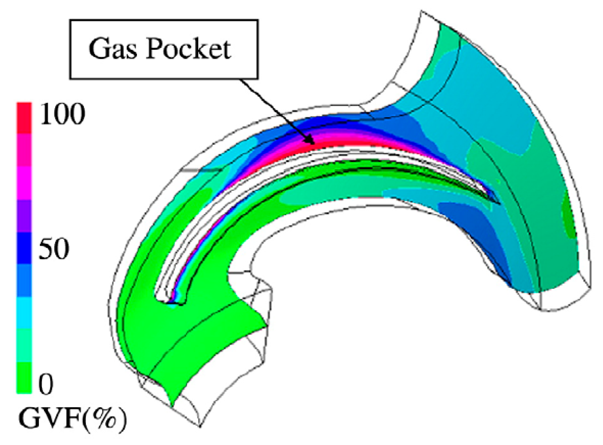
Sekoguchi et al. [58]Transparent casing
electric resistivity probe
The evolvement of dispersed bubble to slug flow and a large gas pocket
Kim et al. [59]Transparent casingPhase slippage leads to bubble agglomeration
Sato et al. [60]Transparent casingBubble flow to separated flow as gas flow rate increases
Takemura et al. [61]Transparent casingBubble accumulation coincided with large pressure gradient
Chisely [62]Transparent casingGas filled space starts to develop at the suction pipe of the pump
Suryawijaya et al. [63]Transparent casingBubble accumulates at pressure side of impeller blade
Estevam [64]Transparent casing1st study of flow patterns in ESP
Poullikkas [65]Transparent casingGas bubbles, gas pocket and blockage of pump flow
Thum et al. [66]Transparent casingLarger accumulation of bubbles is observed at pressure side than suction side, four flow patterns: bubble, plug, slug and stratified flow
Barrios [39,67]Transparent casingBubbly flow and segregated flow are observed
Gamboa [40]Transparent casing1st study of flow pattern map in ESP impeller
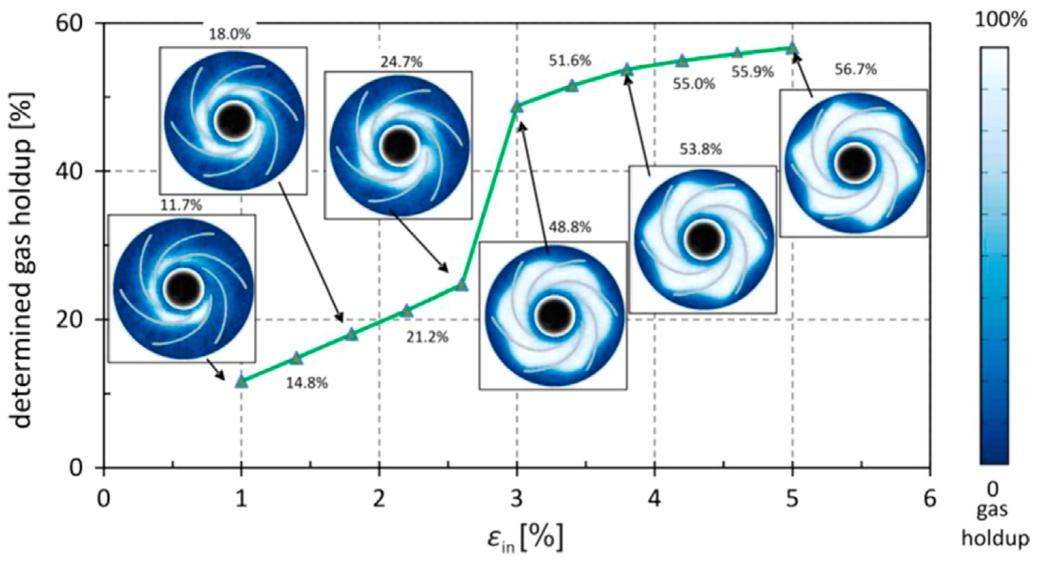
Schäfer et al. [68]HireCT, non-intrusiveMeasurement of gas void distribution in multiphase centrifugal pump
Neumann et al. [69]HireCT, non-intrusiveMeasurement of gas void distribution in multiphase centrifugal pump
Verde et al. [70]Transparent casingFlow patterns in ESP: bubble, agglomerated bubble, gas pocket, segregated flow
Table 9. Correlations of surging initiation (1st transition boundary) in literature.
StudyCorrelationApplication Range
Turpin et al. [78] ϕ = ( 2000 3 P i ) Q G Q L ϕ —empirical constant
Pi < 2.8 mPa
Cirilo [33] λ C = 0.0187 P i 0.4342 Pi < 3.4 mPa
QL < 0.02 m3/s
Estevam [64] λ C = 31.92 32.15 ( 1 λ G )
Duran [37] Q G Q max = ( 5.58 ρ G ρ L + 0.098 ) ( Q L Q max ) 1.421 Pi < 2.4 mPa
QG < 0.02 m3/s
QL < 0.013 m3/s
Zapata [38] Q G Q max = 0.027 Q L Q max 0.9001 Q L Q max Pi < 1.4 mPa
QG < 0.02 m3/s
QL < 0.016 m3/s
Gamboa and Prado [72] Q G Q max = ( ρ G ρ L ) 0.2 ( Ω D 2 ν ) 0.4 ( 0.102 exp ( Q L Q max ) ) 4.4682 Pi < 1.7 mPa
Zhu et al. [44] λ C = 2 [ 0.4 σ ( ρ L ρ G ) Ω 2 R I ] 1 2 10.056 ( σ ρ L ) 3 5 ( Δ P Q L ρ L V ) 2 5 ( ρ L ρ G ) 1 5

