An Integrated Start-Up Method for Pumped Storage Units Based on a Novel Artificial Sheep Algorithm

School of Hydropower and Information Engineering, Huazhong University of Science and Technology, Wuhan 430074, China
*
Authors to whom correspondence should be addressed.
Energies 2018, 11(1), 151; https://doi.org/10.3390/en11010151
Submission received: 22 November 2017
/
Revised: 12 December 2017
/
Accepted: 19 December 2017
/
Published: 8 January 2018
Abstract
:Pumped storage units (PSUs) are an important storage tool for power systems containing large-scale renewable energy, and the merit of rapid start-up enable PSUs to modulate and stabilize the power system. In this paper, PSU start-up strategies have been studied and a new integrated start-up method has been proposed for the purpose of achieving swift and smooth start-up. A two-phase closed-loop startup strategy, composed of switching Proportion Integration (PI) and Proportion Integration Differentiation (PID) controller is designed, and an integrated optimization scheme is proposed for a synchronous optimization of the parameters in the strategy. To enhance the optimization performance, a novel meta-heuristic called Artificial Sheep Algorithm (ASA) is proposed and applied to solve the optimization task after a sufficient verification with seven popular meta-heuristic algorithms and 13 typical benchmark functions. Simulation model has been built for a China’s PSU and comparative experiments are conducted to evaluate the proposed integrated method. Results show that the start-up performance could be significantly improved on both indices on overshoot and start-up, and up to 34%-time consumption has been reduced under different working condition. The significant improvements on start-up of PSU is interesting and meaning for further application on real unit.
1. Introduction
Nowadays, the increase of energy demand and the depletion of fossil fuel have necessitated the large-scale utilization of renewable energy (RE). More and more REs, like wind and solar power have access to power grid [1]. Due to the intermittent of the wind and solar power, the stability of the power grid that contains large capacity of RE has become a severe problem. Energy storage devices like batteries [2,3], flywheels [4] and pumped storage units (PSUs) [5] are indispensable in RE- connected power systems to mitigate this problem. Among these, PSUs might be the most economical and mature tool for power storage [6]. In addition, PSUs have good performance in peak load shaving, frequency regulation and emergency response in power systems [7]. In recent years, with the increasing scale of RE-integrated power systems, a considerable amount of work [8,9,10,11] has been carried out to study large-scale pumped storage facilities integrated with the grid-connected wind or solar power systems. In [8], joint operation of REs and energy storage devices like PSUs is studied in the energy and ancillary service market. In [9], the scheduling problem of a hybrid energy system containing intermittent solar power and pumped hydro storage (PHES) system has been investigated. In [10], a flexibility-based reserve scheduling method for energy storage system with PSUs has been developed to improve the flexibility of the power system. In [11], a model for transient stability analysis of a combined wind-pumped storage generation system is studied. Furthermore, this new generation model will be installed in El Hierro Island, in Spain. In those system or facilities where PSUs have been extensively adopted, the control quality of PSUs could not be neglected.
As a kind of hydropower generating unit, one of the merits of PSUs is their quick start-up, while a PSU could start and transfer to no-load condition from static status within 100 s and increase the power output to rated value within several minutes. This merit makes it able to quickly respond to RE power intermitting and load fluctuation, and keep the stability of the power system containing large-scale RE. The unit start-up related problems have attracted great interest of researchers. In [12], Saboya et al. proposes a start-up decision method by using machine learning-based system for providing secondary frequency control for a power grid. In [13], experimental investigations of transient pressure variations in a high head Francis turbine during start-up. A control system model of a hydropower unit was built and the start-up process was simulated in [14].
PSU start-up usually refers to the process of unit starting in turbine mode. This process begins at the time the guide vane is beginning to move and ends at the time the unit connects to the grid. PSU start-up is a complex control problem. Multiple control models exist in start-up processes. The traditional and actually applied start-up strategy of PSUs mainly contains two phases [15], namely the open-loop type and the close-loop type [16]. In the first phase, a direct guide vane control (DGVC) is adopted, which is usually open-loop, while the governor drives the guide vane (GV) as a given law. In the second phase, a closed-loop PID control is applied to track the rated rational speed and maintain the stability. The open-loop DGVC law provides the trajectory of guide vane opening (GVO), which could be a one-stage polyline or two-stage polyline. Take the two-stage DGVC as an example, in a two-stage strategy, the guide vane will firstly open to start opening, which is about twice as much as the no-load opening, and then keep the opening for a while; until the rotational speed rises to a threshold, guide vane opening is adjusted to the no-load opening. In the second phase, a closed-loop PID control is switched in to stabilize the rotational speed as soon as it reaches a threshold value.
Although the traditional strategies are applicable, there are two main drawbacks, which are: (1) parameters of GVO trajectory in the open-loop DGVC are difficult to set, which are always selected by experience; (2) study on optimization of start-up strategy is not sufficient. In order to handle these problems, researches have tried efforts. Bao et al. designed an “open-closed loop” GVO trajectory and the results indicated that a fast and smooth start-up process could been achieved [17]. Zhang et al. proposed a new DGVC strategy, which integrates the open-loop and close-loop trajectories in DGVC, aiming at balancing the start-up time and control quality [18]. In [7], Yang and Yang tried to modify the conventional open-loop DGVC law and the improved strategy has proved to be effective in promoting start-up performance. Besides, more efforts have been made in optimization of start-up strategies. Zhou et al. [19] selected a constant rational speed growth rate as the objective, so it’s easier to control the frequency change in the whole start-up process. The results also indicate that indices of rotation torque, axial thrust fluctuation as well as the pressure fluctuating of penstock could be improved except for the quick-start index. Dynamic control indices have been chosen as optimization objectives in designing an adaptively fast fuzzy fractional order PID controller in the second phase of start-up process and the simulation results demonstrates that the new controller could enhance the dynamic performance and stability of the pumped storage unit governing systems in the start-up process [20]. Although control quality indices are often considered in start-up strategy optimization, the start-up time is always neglected. An excellent start-up strategy should be built on indices concerning both quickness and control quality. Pannatier et al. presented the start-up and synchronization procedures of large variable-speed pump-turbine units in pumping mode. By the optimization of the start-up time, it leads to a significant decrease of the start-up time [21].
As for parameter tuning for control system of hydropower generating units, meta-heuristic algorithms have been successfully applied [22,23]. Moreover, some popular meta-heuristic algorithms, such as Genetic Algorithm (GA) [24], particle swarm optimization (PSO) [25], Ant Colony Optimization (ACO) algorithm [26], and Gravitational Search Algorithm (GSA) [27,28,29] have been adopted to solve optimization problems. Although numerous meta-heuristic algorithms have been proposed and applied to solve different optimization problems, there is no specific algorithm which can solve all optimization problems. For optimization of start-up strategy, a powerful algorithm is essential to achieve the desired goal.
Flocks of sheep, which is a common swarm in nature, also show intelligence in social activities. In foraging ground, the strolling of sheep implies individual exploration, and the bellwether is the leading elite that affects the swarm movement. Many swarm intelligence (SI) techniques are inspired by foraging and search behaviors. However, there is no SI technique in the literature mimicking the Herding Effect, which is a well-known phenomenon in the sheep flock. Motivated by this interesting behavior, a new meta-heuristic optimization algorithm is proposed in this paper. The mathematical model of the social behavior of a sheep flock, as well as investigation of its abilities in solving benchmark problems, will be fully discussed before applying it in start-up strategy optimization of PSU.
Motivated by the above discussion, a new integrated start-up method for PSU is proposed in this paper, while a two phase’s closed-loop startup strategy is designed, and optimization scheme is built for parameter optimization of the strategy. Moreover, in order to promote the optimization performance, new meta-heuristic algorithm is studied. This paper presents a novel meta-heuristic called Artificial Sheep Algorithm (ASA) based on social behaviors of sheep flock. The mathematically model of the social behavior of sheep flock, as well as investigation of its abilities in solving complicated problems, will be fully discussed.
The remaining part of this paper is organized as follows: Section 2 establishes a mathematical of Pump-Turbine Governing System which composed of PID controller, governor servo-mechanism, water diversion system, pump-turbine and generator. Section 3 introduces the theoretical knowledge of ASA. Section 4 delineates specific operations of traditional start-up and the proposed integrated start-up strategy. In Section 5, the performances of optimization schemes and integrated start-up strategy are analyzed by comparison experiment. The conclusions are summarized in the Section 6.
2. Modelling of Control System of PSU
The pump-turbine governing system (PTGS) is a main control system that undertakes the modulation of frequency (rotational speed) and power output. The simulation of PSU start-up is also related to PTGS. PTGS is composed of governor controller, governor servo-mechanism, water diversion system, pump-turbine and generator, as presented in Figure 1. In this paper, a method of characteristic (MOC) and an improved Suter transformation method have been studied for the modelling and simulation of PTGS [30,31].
2.1. Modelling of Water Diversion System
In this paper, the fundamental equations are applied to describe the water diversion pipelines, as shown below [32]:
The details of all the symbols in these equations are given in the nomenclature. The method of characteristics (MOC) is applied to the partial differential equations (PDEs) as shown in Equations (1) and (2), and the partial differential terms associated with the flow velocity and the pressure are reduced to ordinary differential ones compatible with two characteristics lines C+ and C− as shown in Figure 2.
The fixed-grid MOC requires that a common time step () being used for the solution of the governing equations in all pipelines [33]. Consider L is one of the pipelines total length subdivided into equal sections N, each of which . If we start with known steady state conditions at t = 0, then we know Q and H at the N + 1 sections of the pipeline. If we specify the time interval defined as the , the characteristic lines from the sections A and B intersect at P [34]. In these conditions, the final equations can be written in the following forms [32]:
where coefficients , .
In addition, the elastic water hammer effect is considered and different forms of pipelines, channels, and surge tanks are included.
2.2. Modelling of Pump-Turbine
Pump-turbines are the key component of PTGS, and the modeling of a pump turbine is based on its complete characteristic curves. The original performance curves of the pump-turbine unit are shown in Figure 3. The “S” area of characteristic curves presents an uneven distribution, crossing and aggregation phenomenon, which brings difficulties for modeling of pump-turbines. In order to overcome these problems, an improved Suter transformation method [35,36] have been proposed, and experiments have proved that the improved Suter transformation method could eliminate the uneven distribution, crossing and aggregation of “S” zone. Different processing methods for the curves can establish the pump-turbine linear model under different conditions as well as a nonlinear model by interpolation or fitting.
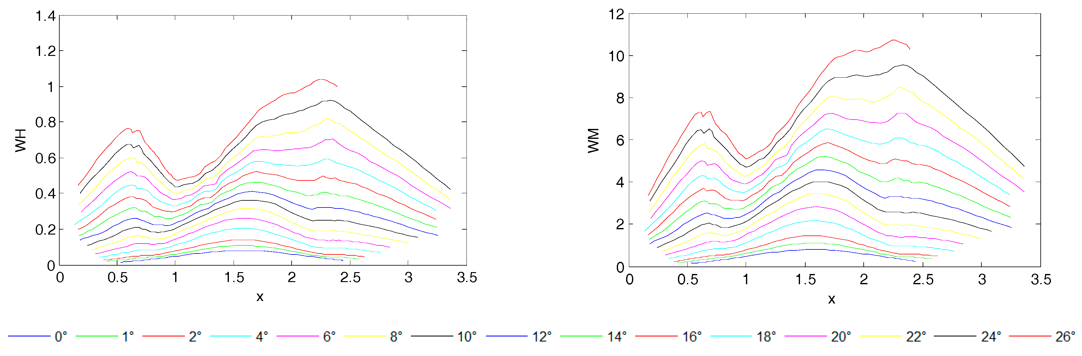
By setting the unit parameters N11~Q11 and N11~M11 as a cross-ordinate, a series of two-dimensional curves could be built to describe the complete characteristics of a pump turbine. While setting the gate opening y as reference variable, the flow characteristic curves and the torque characteristic curves of the complete characteristics could be established for a pump-turbine, as shown in Figure 3. In this figure, the range of guide vane opening is from 0° to 26°. From Figure 3, it can be noticed that the “S” area exists in characteristic curves. A multiple-valued problem occurs in interpolation calculating for pump-turbine modeling. In order to overcome this obstacle, an improved Suter transformation is used, as follows [36]:
where, , k2 = 0.5~1.2, Cy = 0.1~0.3, Ch = 0.4~0.6. A transformed WH and WM curves based on the improved Suter transformation method have been shown in Figure 4. It is obvious that the improved Suter transformation method eliminate the “S” characteristics, the uneven distribution, cross and aggregation of the curves.
According to the above content, the calculation model of pump-turbine could be summarized as Equation (6):
where equations hn+1 and mn+1 represent the interpolation of the characteristic curves of the pump turbine unit.
2.3. Modelling of Power System
This model calculates the unit running speed from the unbalance between the load moment Mg and the shaft mechanical moment Mt as defined in follows [37]:
Under start-up operation, the value of Mg is 0 and the corresponding equation can be considered as a special case of Equation (7), as follows:
2.4. Modelling of Pump-Turbine Governor
The pump-turbine governor contains a controller and servomechanism. A conventional PID controller is often used to eliminate the speed deviations from a reference speed in the later phases of a start-up process and under no-load conditions [38]. The transfer function of a PID controller is described as:
and the output of the controller is shown as:
where Kp, Ki and Kd are the proportional gain, integral gain, differential gain of PID controller. u(s), aref (s) and a(s) are the Laplace transform of controller output u, reference speed aref and synchronous generator speed a.
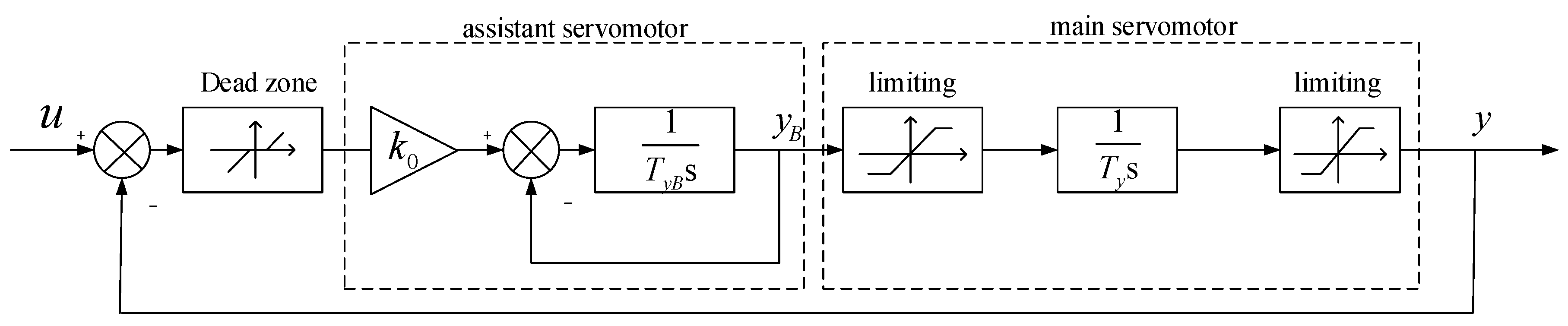
The servomechanism is the actuator of the speed governor which consists of main and assistant servomotors. The servomechanism is used to amplify the control signal and provide power to operate the guide vane of a pump-turbine. The structure of the servomechanism is shown as Figure 5.
2.5. Simulation of PTGS
While simulating the PTGS, the coupling relationships of water diversion system, pump-turbine and generator should be considered. Thus the iterative computation to calculate the water flow Qn+1 and turbine speed Nn+1 of the next time n + 1 for the simulation of PTGS before switching PID regulation is adopted, as the flow chart shown in Figure 6.
3. Artificial Sheep Algorithm
Optimization of parameters in the start-up strategy is an important task in this paper. A novel meta-heuristic called Artificial Sheep Algorithm (ASA) based on the social behaviors of sheep flocks is proposed and used to optimize the parameters. A series of test experiments are conducted to evaluate the performance of the proposed ASA.
Sheep flocks are always regarded as a scattered organization. Although they are loose, and can collide with each other in group activities, they have the habitual nature of following and moving towards the bellwether who is the strongest in the group. As sheep appear to blindly follow, people always associate them with conformity. Actually, the behavior of this social group has undergone ten million years of natural testing. From the perspective of SI, the loose individuals indicate random diversity, the blind herd behavior indicates high-efficiency positive feedback, and the bellwether leading implements the sharing of information in the whole group. This paper is inspired by the herd behavior of sheep flock and tries to simulate a novel meta-heuristic optimization algorithm with some artificial measures.
The social behaviors of sheep flock are attractive, and two main behaviors, namely the free strolling of individuals and strong leading of bellwether. In a sheep flock, the strongest sheep is called the bellwether, acting as the leader of the swarm. When fleeing from a predator or foraging, the individual will follow the bellwether by moving as close as possible. When strolling or playing, individuals are loose and always move randomly in their own local region.
3.1. Theoretical Knowledge of Algorithm
Consider a sheep flock with N sheep, the position of the ith sheep at specific time “t” is defined as:
where represents the position of ith sheep in the dth dimension, D is the dimension of the position.
For solving a minimization problem:
where is the lower boundary of the searing space, and is the upper boundary of the searing space. The objective function value of the ith agent at time “t” is expressed as .
Leading of bellwether
The influence of the bellwether is decisive. When the bellwether moves with a big stride, individuals will adjust their motion trajectory to follow the bellwether closely. The position of the bellwether should be recorded and inherited, and this position is denoted as . The influence of the bellwether acting on the ith sheep is expressed as bellwether vector, denoted by .
The bellwether vector that affects the movement of the ith agent, i = 1, …, N, is defined as:
where is the influence scope of the bellwether playing on the ith sheep on the dth dimension, , , is the coefficient of leading scope, rand1 is a random number generated in [−1, 1], w is a dynamic weight that linearly decreased from 1 to 0 over the course of iterations.
The coefficient c1 is a random value whose center is 1, and its radius is determined by the parameter , which is selected from [0, 1]. The is a control parameter, which influences the consensus effect of the bellwether in defining the distance vector. When tends to 1, it emphasizes the consensus influence of the bellwether; when tends to 0, it enhances the stochastic components. The coefficient c2 is a random dynamic number that is automatically generated, and its random range is linearly decreased over the course of iterations.
Individual strolling
Every individual of flock forages autonomously in a local area, and this behavior is called “self-awareness”. The mathematical model of “individual strolling” to represent shelf-awareness of sheep individual in the process of foraging is proposed as follow. We define a location vector to denote self-awareness in foraging.
The shelf-awareness vector that affects the movement of the ith agent, i = 1, …, N, is defined as:
where is a random number generated from [0, 1], the term is used to generate periodic random.
The vector represents the self-driven behavior and local random search of a sheep, which consists of a series of nonlinear operations. The parameter is a positive number that modulates the amplitude of the strolling step. As increases, the sheep’s jump steps increase exponentially and vice versa. As a result, this parameter controls the resolution of individual exploration. The value of should be chosen according to the search scope of the optimization problem.
In a sheep flock, the direction of the sheep flock is determined by the lead of the bellwether and the autonomous foraging. Based on the discussion above, the movement of a sheep is affected by its self-awareness and the summoning of the bellwether. The individuals in artificial sheep flock will automatically update their positions as follows:
where is linearly decreased from 1 to 0 over the course of iterations and r3 is random number generated in [0, 1].
Competition strategy
In ASA, competition mechanism is designed to keep the diversity of the flock. For a minimum problem, at a specific time “t”, calculate the average value of N objective function values of the flock , and the minimal objective function value .
For the ith sheep, if the elimination criteria as following is satisfied:
Then, the ith sheep is eliminated and reinitialized between .
3.2. The Optimized Procedures of Algorithm
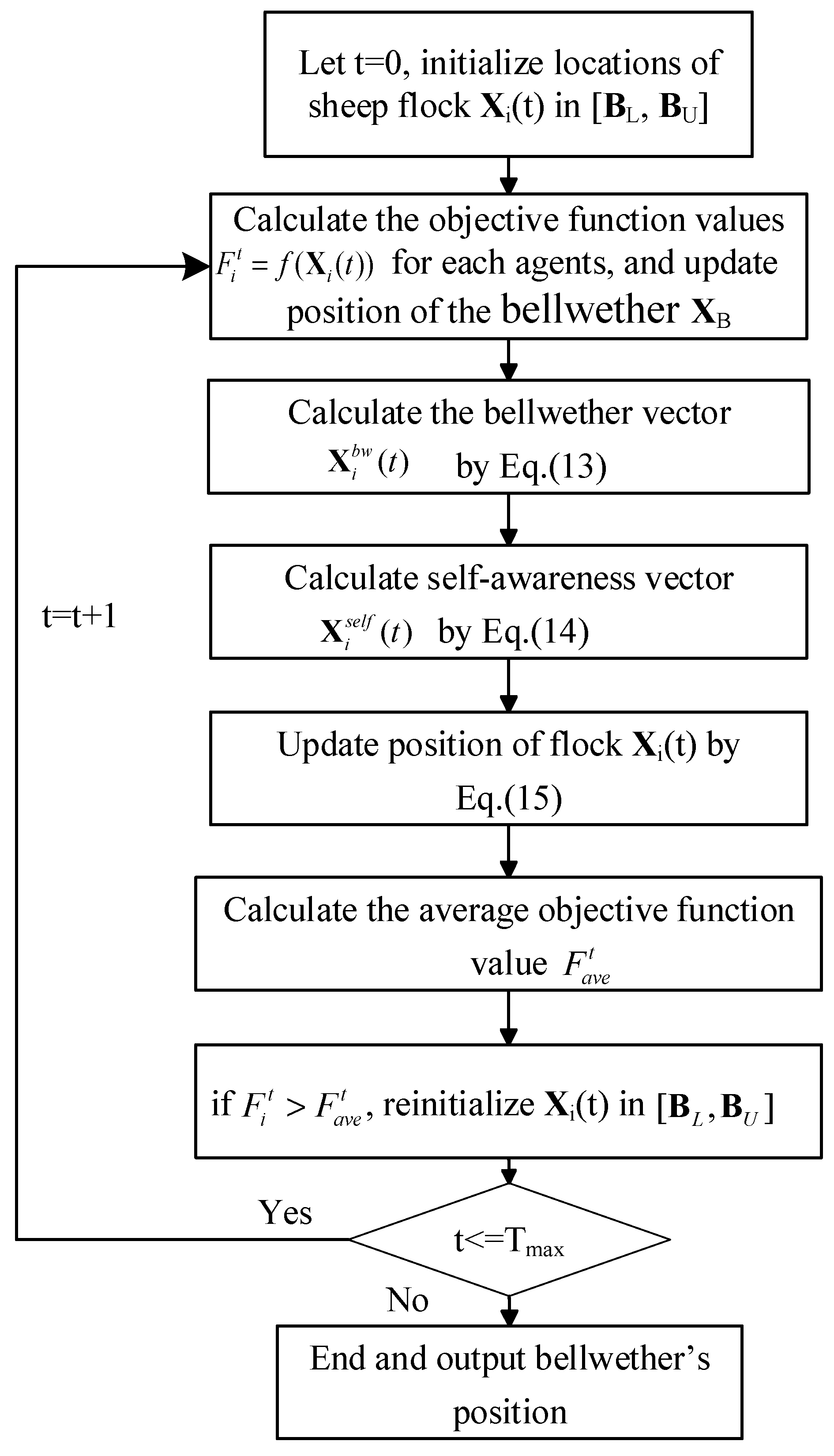
The whole idea and the specific architecture of ASA have been clearly presented in above paragraphs. The flow chart of ASA optimization is illustrated in Figure 7. Accordingly, the main steps of the ASA is summarized as follows.
- Step 1: Initialization. Initialize locations of sheep flock with N sheep in the solution space with boundaries , and calculate the objective function value , i = 1,…,N; set the first sheep as the bellwether ; set other control parameters: the initial scope coefficient of leading and the modulation coefficient of strolling ; set the total number of iteration T, and the current number of iteration t = 0.
- Step 2: Calculate the objective function values of agents , i = 1,…,N, and update the bellwether by conducting: if then , .
- Step 3: Calculate the bellwether vector , i = 1,…,N, according to the Equation (13).
- Step 4: Calculate self-awareness vector , i = 1,…,N, according to the Equation (14).
- Step 5: Updating position of flock according to the Equation (15).
- Step 6: Judge whether sheep need to be eliminated according to the Equation (16) and reinitialize the same number of new sheep between .
- Step 7: t = t + 1; if t > Tmax, end and output bellwether’s position as the final solution; else, go to Step 2.
The ASA is inspired by the behavior of the sheep flock and the complete optimization mechanism of ASA algorithm has been established now.
3.3. Experimental Study and Comparison Results on Benchmark Functions
To evaluate the performance of the proposed ASA, as well as other seven meta-heuristic optimization algorithms, i.e., Particle Swarm Optimization (PSO) [25], Differential Evolution (DE) [39], Ant Colony Optimization for continuous domain (ACOR) [40], Artificial Bee Colony (ABC) [41], Cuckoo Search (CS) [42], Gravitational Search Algorithm (GSA) [27], and Grey Wolf Optimizer (GWO) [43], were applied to solve 13 standard benchmark functions. The selected algorithms are representatives of evolutionary, physics-based and SI based meta-heuristics. In these algorithms, the newly developed meta-heuristics are included. The following experiments are conducted on MATLAB (R2016a, MathWorks, Natick, MA, USA).
3.3.1. Benchmark Functions
Table 1 and Table 2 present the benchmark functions used in our experimental study. The employed benchmark functions can be divided into two groups: unimodal, multimodal test functions with high dimension. The unimodal test functions have only one global optimal value, so they are often used to test the ability of exploitation of algorithms, as shown in Table 1. The multimodal test functions with high dimension have many local optimal values expect for the global optimum, so they are most difficult to optimize, as shown in Table 2.
In these tables, D is the dimension of function, fopt is the minimum value of the function, and searching space is a subset of . The minimum value (fopt) of the functions of Table 1 and Table 2 are zero, except for F8 which has a minimum value of −418.9829 × D. The optimum location (Xopt) for functions of Table 1 and Table 2, are in [0]D, except for F5, F12 and F13 with Xopt in [1]D and F8 in [420.96]D.
3.3.2. Parameters of Algorithms
A set of fair parameters obtained by a simple trail-and-error procedure was adopted for ASA. For a fair comparison, the recommended parameters of PSO, DE, ACOR, ABC, CS, GSA and GWO were used to tackle these problems. In order to conduct a fair comparison, the maximum number of iteration was chosen to 1000 and the population size of all algorithms was set to 30 (i.e., N = 30) in all experiences in this section. Other parameters of the comparative algorithms were set as follows:
- PSO: the inertia weight w was decreased linearly from 1 to 0.2. c1 and c2 are learning genes and chosen to be 2 in this section in this paper [44].
- DE: the mutation factor , the crossover rate [44].
- ACOR: the number of ants used in an iteration m = 3, an archive size k = 50, the Locality of the search process, q = 0.05 and the speed of convergence, E = 0.85 [44].
- ABC: the number of onlooker bees, employed bees and food sources was 30 [44].
- CS: the discovery rate p = 0.25 [42].
- GWO: are linearly decreased from 2 to 0 over the course of iterations and r1, r2 are random vectors in [0, 1] [43].
- ASA: the initial scope coefficient of leading ; the modulation coefficient of strolling .
3.3.3. Comparison Results on Benchmark Functions
All experiences were repeated 30 times independently. The mean value, the best value, as well as the standard deviation, of the optimal objective function values of 30 runs, were reported for unimodal functions in Table 3 and for multimodal test functions with high dimension in Table 4.
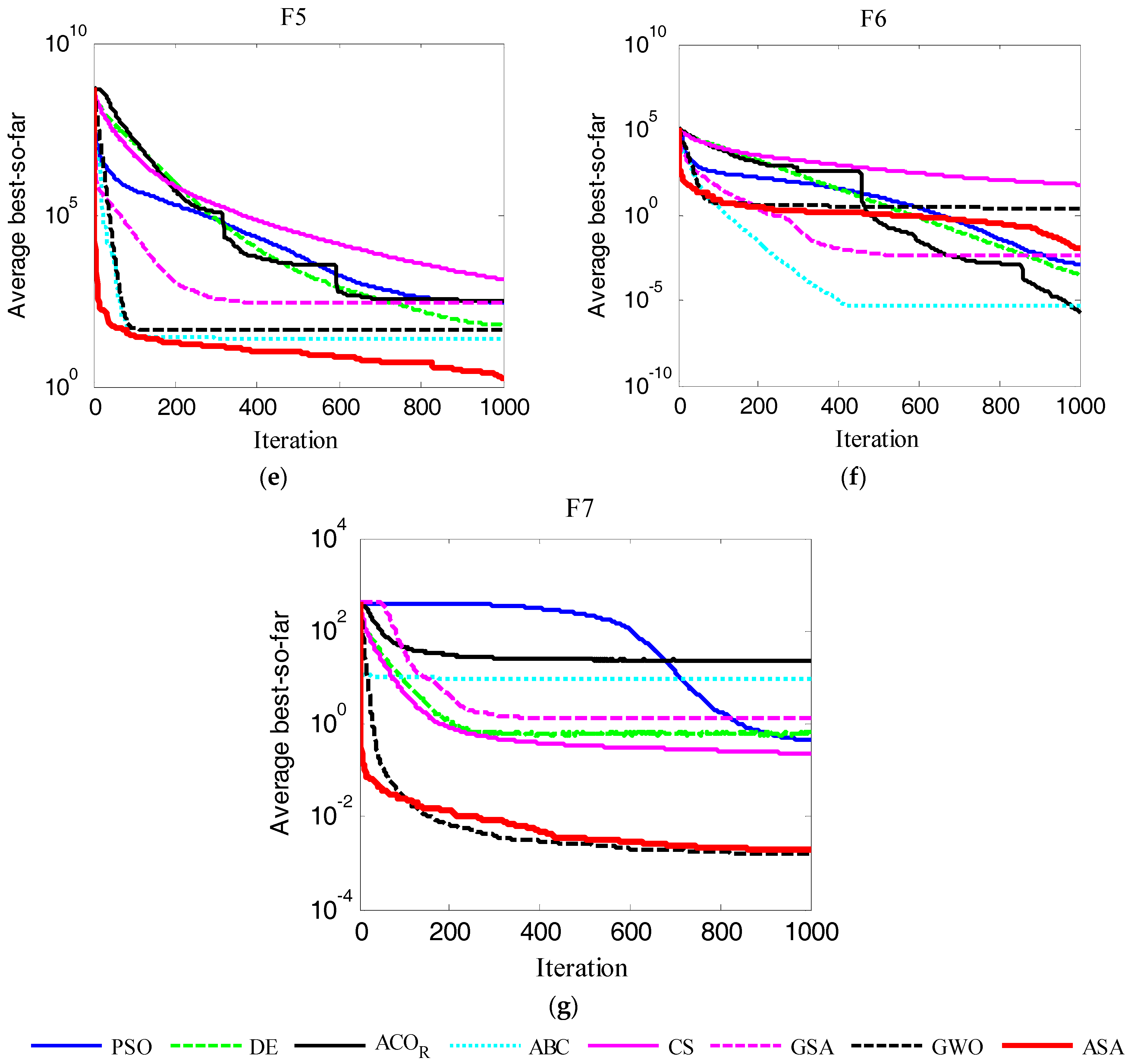
The unimodal test functions are relatively simple to optimize because they only have one global optimal value. From Table 3, it is clear that the ASA has a very good performance for the unimodal test functions. The ASA algorithm shows obvious advantage over the competitors in the remainder of high dimension unimodal functions, except for F4 and F6. The multimodal test functions with high dimension are relatively difficult to optimize because they have many local optimal values and one optimal global value. The ASA also has significant performance, as shown in Table 4. Generally, the ASA algorithm has shown an obvious advantage over the competitors on high dimensional benchmark functions F1–F13. Furthermore, optimization processes of the comparative algorithms were given in Figure 8 and Figure 9. The values shown in these figures were the average of “best so far” in iterations achieved from 30 runs. The “best so far” is the best objective function value searched by the artificial sheep flock at certain iteration.
Figure 8 shows the average “best so far” in iterations obtained by the eight methods on the unimodal functions F1–F7. From Figure 8 ASA performance is superior to the seven methods in the optimization process on all high dimensional unimodal functions except for F4 and F6.
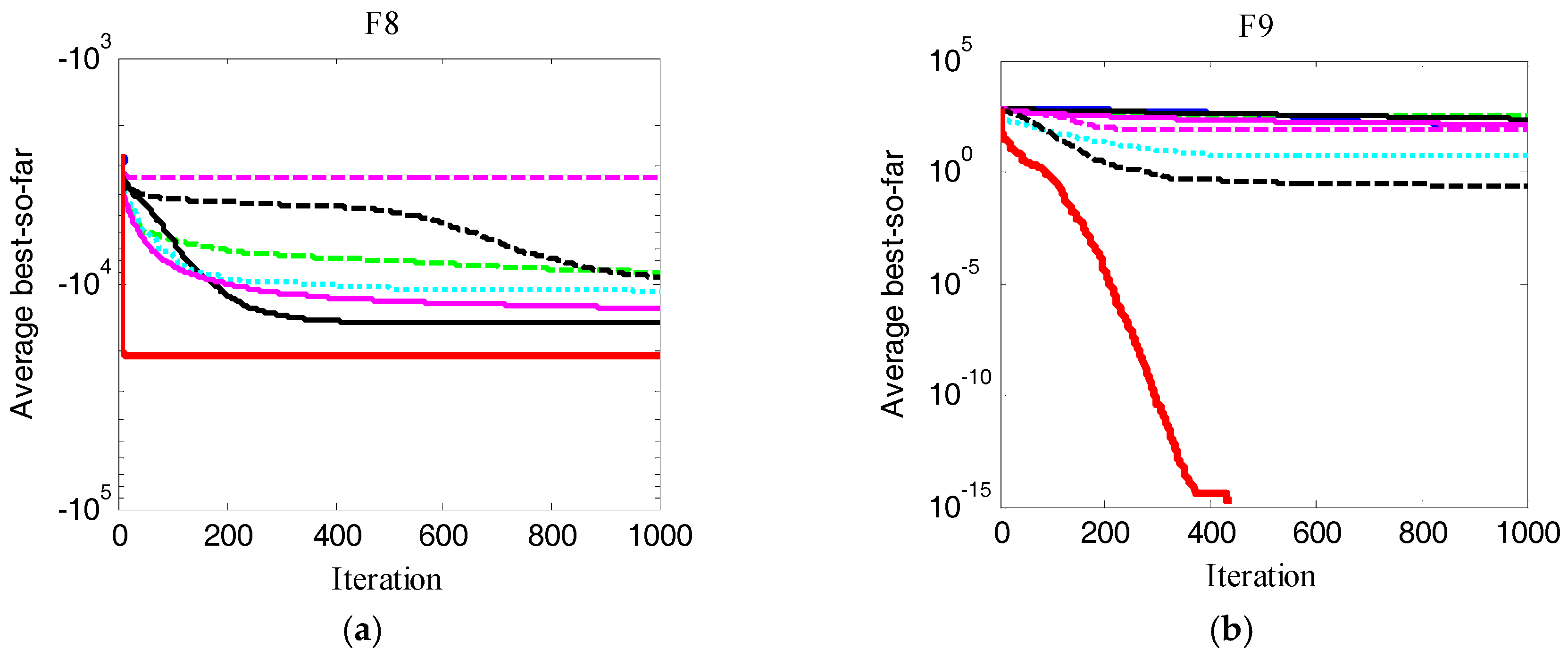
Figure 9 shows the average iteration processes obtained by the eight methods on the multimodal functions F8–F13. From Figure 9, it is demonstrated that ASA performs the best compared with another seven methods on F8–F12. ASA has advantages over other algorithms, except for DE, in the optimization process of F13. From these figures, it was seen that the ASA had a faster converge speed compared with other approaches. In particular, ASA had a very good performance on high dimensional test functions.
4. An Integrated Start-Up Method for Pumped Storage Units
4.1. Traditional Start-Up Strategies of a PSU
The traditional start-up method of a PSU contains two phases. In the first phase, the control system of the PSU is open-loop, in which the feedback signal of rotational speed of pump-turbine is not adopted and used for control. In this phase, the control system undertakes a kind of direct guide vane control (DGVC). After receiving the start-up command, governor will control the guide vane to tract a DGVC trajectory. As the rational speed of pump-turbine increase to a threshold value, the second phase starts. At that moment, the control system is closed-loop, while the feedback signal of pump-turbine speed is used for control. The system is then under a speed control mode. In the second phase, PID control is adopted for the purpose of adjusting and maintaining the stability of pump-turbine speed referring to the rated speed.
4.1.1. The First Phase: Direct Guide Vane Control
One-stage DGVC
The guide value opens as the highest speed to no-load opening, while the rotational speed of unit will increase. As the speed reaches 90% of the rated value, a closed-loop PID control will be switched on to adjust and maintain the stability of speed for grid connection. The one-stage DGVC is illustrated in Figure 10.
Two-stage DGVC
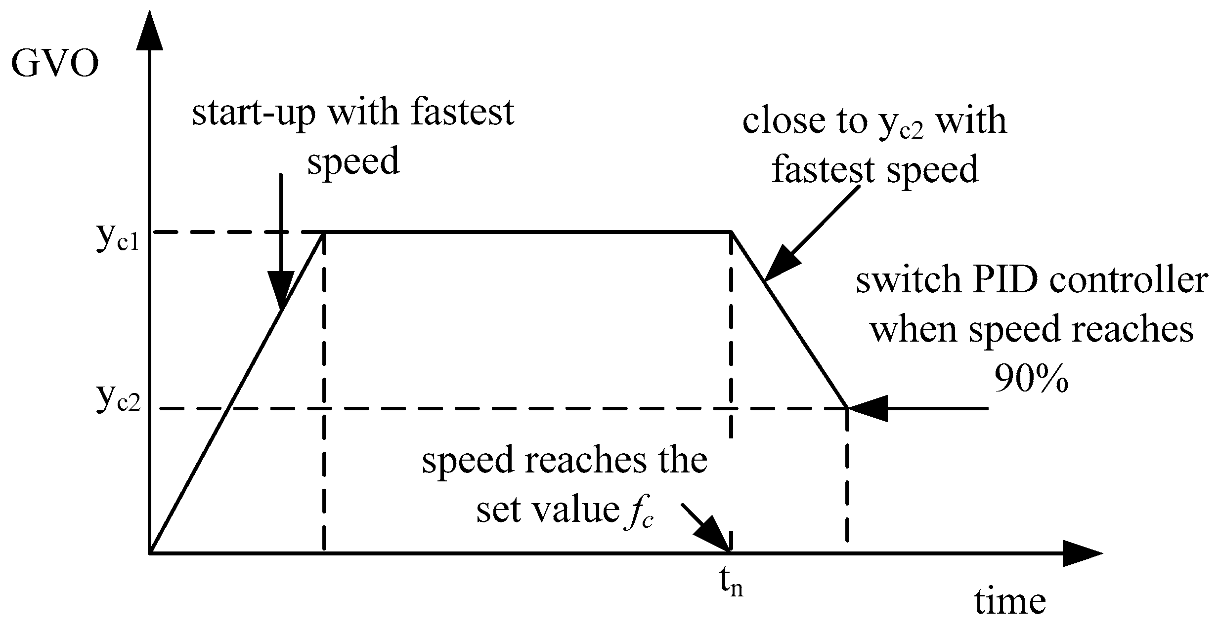
The guide vane opens rapidly to start opening (opening is about twice as much as the no-load opening) with the fastest speed, and keep the opening for a period, until the speed rises to a set value nc (nc is usually 60% of the rated speed). The guide vane opening is then adjusted to the no-load opening immediately. After the speed reaches 90% of the rated value, the PID control is switched on. The illustration of the two-stage DGVC is shown in Figure 11.
4.1.2. The Second Phase: PID Control
As mentioned above, following the open-loop direct guide vane control, the closed-loop PID control will be switched on when the pump-turbine speed reaches a threshold value, which is usually set as 90% of the rated speed. Though the PID controller is a very traditional design, it is still one of the favorite and most widely used controllers for many industrial process control applications. This is due to its simple structure, satisfactory control effect and acceptable robustness [45,46]. The PID controller is easier to understand due to intuitive simplicity of the algorithm and simple meaning of its tuning parameters proportional (Kp), integral (Ki) and derivative (Kd).
In the following, the start-up strategy composed of open-loop one-stage DGVC and closed-loop PID control is named the one-stage start-up strategy. The start-up strategy composed of open-loop two-stage DGVC and closed-loop PID control is named the two-stage start-up strategy.
4.2. Optimization Variables for Start-Up Strategies
In order to improve the start-up performance, the parameters in the start-up strategies could be optimized. Traditionally, PID control parameters are often optimized to enhance the control performance for a quick and smooth PSU start-up. The tuning parameter vector for a PID controller is .
The parameters of the DGVC could also be optimized, though this has seldom been researched. For a one-stage DGVC, the maximum value yc and the rising slope of guide vane kc can be used as parameters to be optimized, as . The parameters to be optimized of a two-stage DGVC are the maximum value of the guide vane opening yc1, the minimum value after guide vane closure yc2 and the set frequency fc when the guide vane began to decrease, as .
In this paper, optimization experiments of the traditional two-phase start-up strategies are grouped into two categories:
Scheme A: optimization of PID controller. In practice, parameters of the DGVC are set as a rule of thumb. The PID parameter vector is optimized. In these categories, one-stage DGVC and two-stage DGVC can be selected corresponding.
Scheme B: optimization of DGVC. DGVC parameters are optimized, the parameters of PID controller are kept the same as the optimized parameters of Scheme A.
4.3. An Integrated Start-Up Method
In order to improve the performance of the start-up process of PSUs, a new integrated start-up strategy and the relevant optimization method are proposed. This strategy is composed of two phases, in which a closed-loop PI control, instead of the open-loop GVO control, is applied in the first phase to open GVO, and a closed-loop PID control is switched on once the speed reaches the threshold. In the first phase, a closed-loop PI control is conducted to open the GVO to accelerate the rotational speed, while the control target is to keep the ratio of differential speed and speed deviation to be a constant:
where dΔa/dt is the speed differential speed; Δa is deviation of speed. When the speed is close to the rated speed (about 98% of the rated speed), the governor will switch to the PID controller to track the rated speed.
Parameters of the integrated start-up strategy can be optimized synchronously. Parameters of the first phase include parameters Kp1, Ki1, of PI controller, and the constant C in Equation (17). Parameters of the second phase are that of PID controller, Kp, Ki, and Kd. Therefore, the optimization vector is .
4.3.1. Objective Function
The objective function for start-up strategy optimization is an integral performance index to evaluate the control performances, including overshoot and start-up time. The Integral Time Absolute Error (ITAE) [47] index is used as the objective function as defined by:
where is parameter vector to be optimized, k is the sample number, Ns is the number of samples, T(k) is the sample time, a(k) is the relative value of unit speed.
In order to assess the performance of the proposed integrated start-up methods quantitatively, three indices about overshoot, start-up time and steady-state error are presented:
amax is the relative value of the peak speed, ts called the start-up time is the corresponding time when the relative value of the speed reaches rated relative speed 1 and the steady-state error means the deviation of the actual rotational unit speed and rated relative speed 1 that can’t be eliminate. Here, considering the constraints of the experiment, we choose the steady-state error at 100 s. The specific description is shown in Figure 12.
4.3.2. Procedures
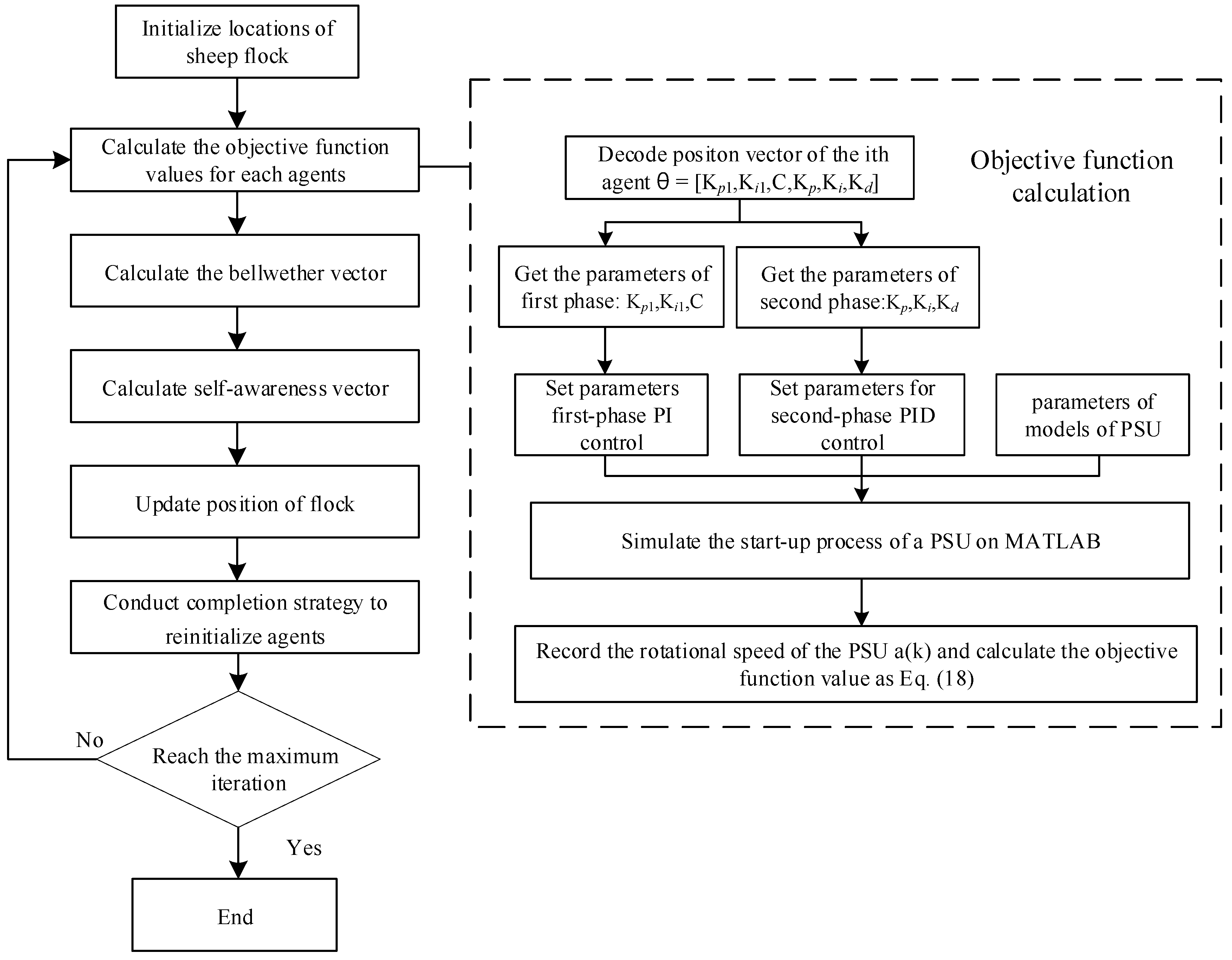
In the proposed method, the ASA is used to optimize the objective function, while optimization parameters are elements in . As for optimization of traditional start-up strategies, i.e., Scheme A and Scheme B, the objective function is also selected as the ITAE function, while the optimization vectors are , , respectively. Take optimization of the integrated start-up strategy as an example, the detail flow chart of start-up strategy optimization based on the ASA is shown in Figure 13. To illuminate the procedures briefly, the main steps are summarized as follows.
- Step 1: Initialization. Initialize locations of a sheep flock with N sheep in the solution space with boundaries , set the first sheep as the bellwether , ; set other control parameters: the initial scope coefficient of leading and the modulation coefficient of strolling ; set the total number of iteration Tmax, and the current number of iteration t = 0.
- Step 2: Objective function calculation. For the ith (i = 1, .., N) agent, the objective function value is calculated as three steps:
- Step 2.1: Decode Xi, and get the control parameters of the first phase Kp1, Ki1, and C, and parameters of second phase Kp, Ki, Kd.
- Step 2.2: Set these parameters for controllers and start the established PTGS simulation plant to simulate the start-up process of PSU; sample and record system outputs including the unit speed a(k), opening of guide vanes y(k).
- Step 2.3: Calculate the objective function value by Equation (18), and let .
- Step 3: Implement other iterative procedures of ASA as described in Section 3.2;
- Step 4: Set, t = t + 1; if t > Tmax, stop simulation and output bellwether’s position as the final solution; or else, go to Step 2.
5. Experiments
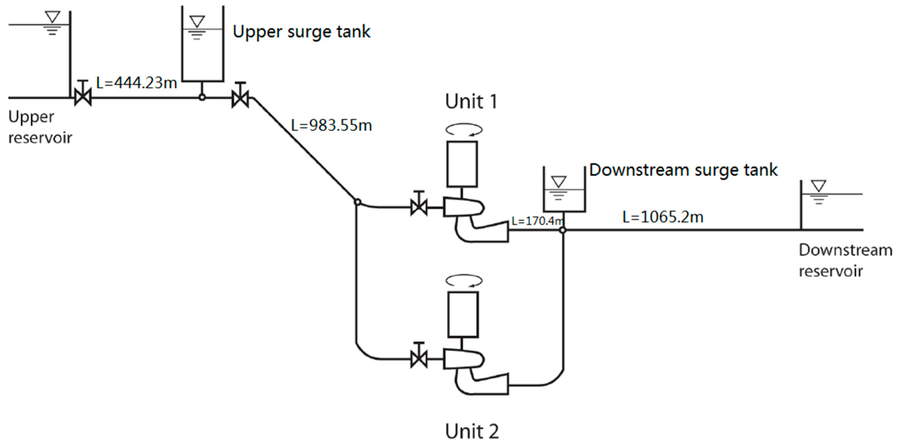
To verify the effectiveness of the integrated intelligent start-up strategy, a PSHP in Jiangxi Province of China has been investigated and used as the study target. The structure of the water diversion system of the PSHP is shown in Figure 14. In this study, the following condition is considered: unit 1 is working and unit 2 stops. The control system of the working PSU is simulated in MATLAB (R2016a, MathWorks, Natick, MA, USA).
5.1. Model Parameters
The values of initial and specified parameters of the simulated PTGS are listed in Table 5, while ts is sampling time. Experiments are conducted under same water head condition which the water level of upper reservoir is 735.45 m and downstream reservoir is 181 m.
As discussed in Section 4, different PSU start-up strategies, including traditional start-up strategies and the proposed one, are optimized by applying ASA. In the following experiments, the parameters of ASA is set as: the initial scope coefficient of leading and the modulation coefficient of strolling , the population size is 30, the total number of iteration Tmax = 200. The boundaries of each optimized parameter are listed in Table 6. Initial DGVC parameters are selected by experience as some popular rules, which are presented in Table 7.
5.2. Comparative Analysis of Traditional Start-Up Strategies
In this part, experiments on optimization of the traditional start-up strategies are conducted. At first, optimization experiments on Scheme A are executed, while one-stage and two-stage DGVC is applied, respectively. In this optimization scheme, the parameters of the first phase DGVC are given by experience, as shown in Table 7, and the second phase PID controller is optimized by ASA.
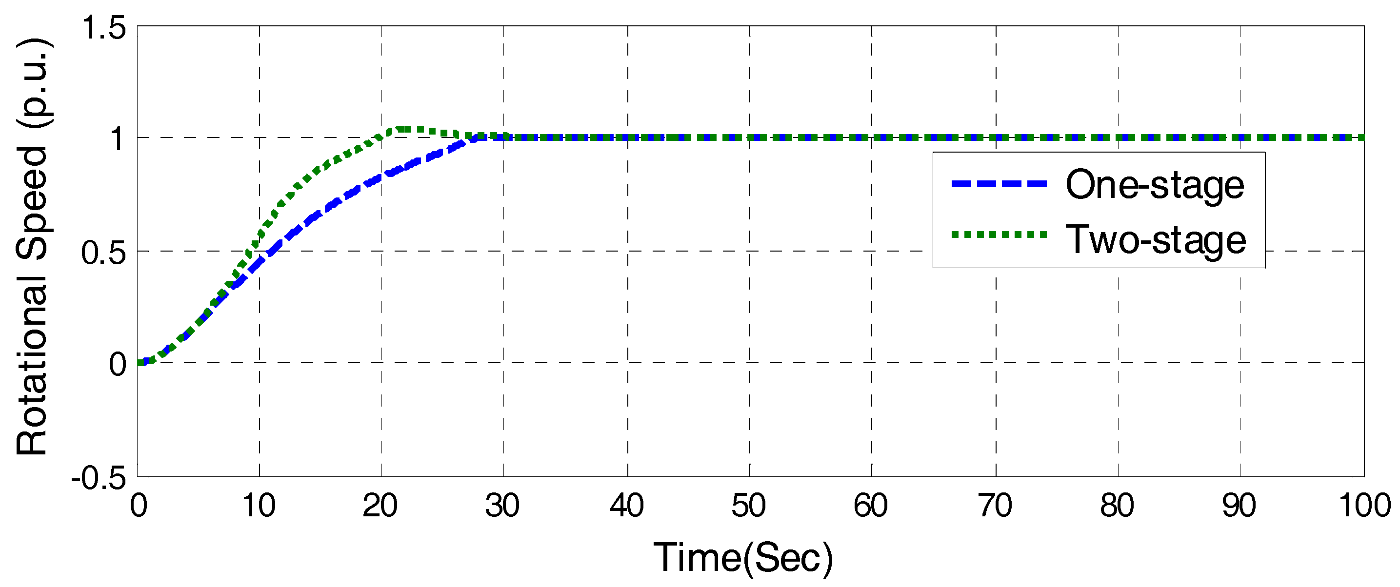
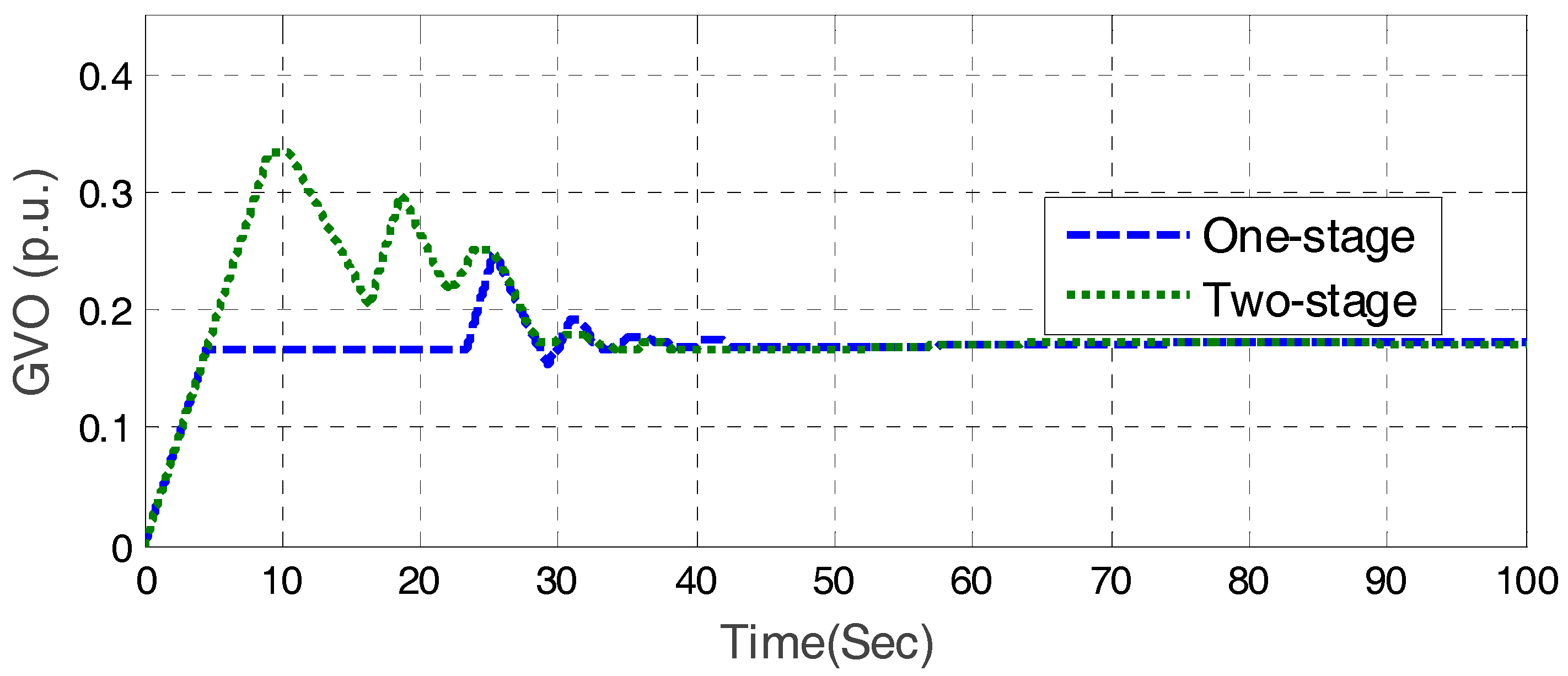
The results of optimized PID controller parameters are listed in Table 8. The dynamic processes of one-stage and two-stage start-up strategies are shown in Figure 15 and Figure 16, where the rotational speed and guide vane opening curves are presented respectively. The performance indices calculated by Equations (19) and (20), including start-up time, overshoot and steady-state error, are listed in Table 9.
From the results in Figure 5 and Table 9, it is found that one-stage strategy achieves a better performance on overshoot at the price of a longer start-up time. Compared to the one-stage start-up strategy, the two-stage strategy possesses a quicker rotational speed rise ratio. From Figure 6, the change process of guide vane opening of one-stage strategy has the same slope with the two-stage strategy to make the rotational speed rises quickly within the first 4.5 s, but the two-stage start-up strategy has a larger guide vane opening as time elapses, therefore, less time is consumed for the rotational speed to reach 90% of its rated value.
Subsequently, one-stage DGVC and two-stage DGVC are compared in experiments on optimization Scheme B, while the parameters of the PID controller are kept the same as in the previous results on Scheme A. In this scheme, the parameters of DGVC are optimized by the ASA.
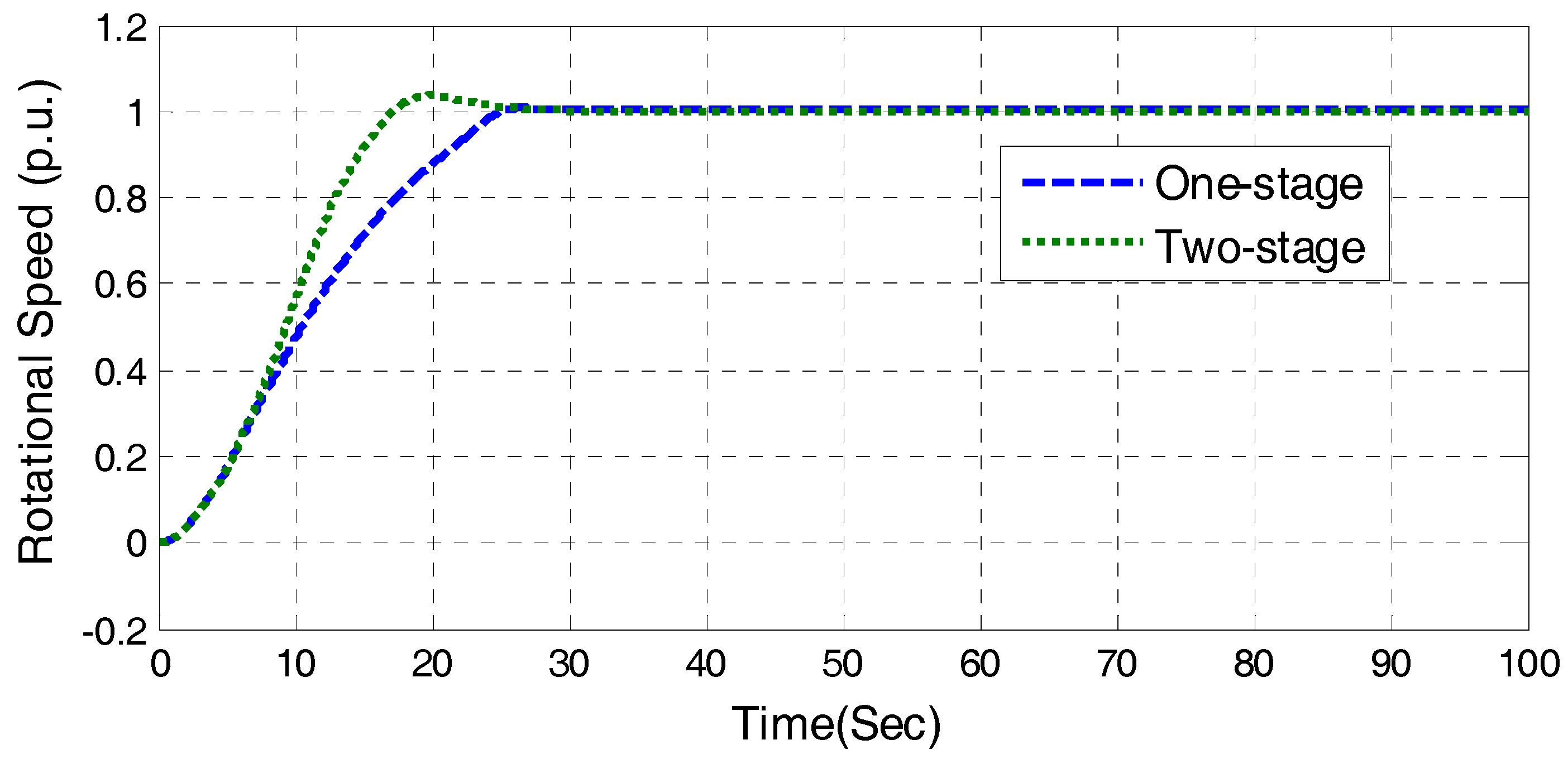
The optimized DGVC parameters are listed in Table 10. The dynamic processes of one-stage and two-stage start-up strategies are shown in Figure 17 and Figure 18, where the rotational speed and guide vane opening curves are presented. The performance indices are listed in Table 11. From these results, a similar conclusion is drawn that a smaller overshoot is obtained with the one-stage DGVC strategy and a shorter start-up time is achieved with the two-stage DGVC strategy.
Some interesting facets are worth discussing. The guide vane responses are similar to those in scheme A. However, in zone A of Figure 18, the guide vane opening doesn’t remain invariant as a horizontal line like in Figure 16. The reason is that the rotational speed increases fast as the guide vane opening continues increasing in this case. The relative value of the speed has risen to 0.64 before guide vane opening reaches the inflection point yc1 = 0.413 to become horizontal. Moreover, point b is the moment the PID controller is switched on and there exists a tiny fluctuation.
5.3. Results of the Integrated Start-Up Method
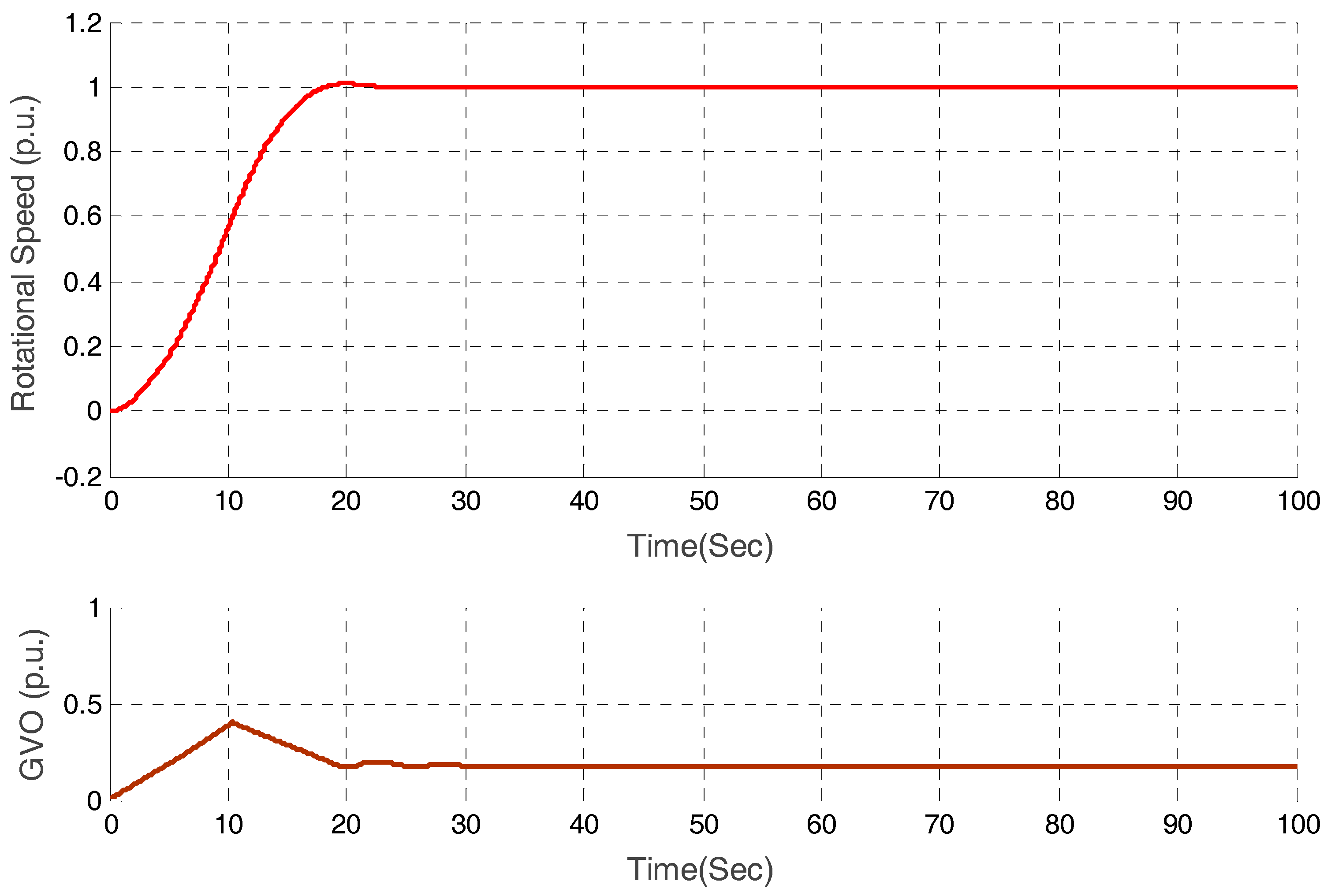
In order to verify the superiority of the proposed integrated start-up method, a comparison of different start-up strategies is made. At first, the results of the integrated start-up method are presented, while the optimized parameters of the integrated method are listed in Table 12, and the corresponding dynamic responses of start-up process are illuminated in Figure 19. From these results, it is obvious that the start-up process achieved by the integrated method shows significant performance improvement, with a short start-up time and negligible overshoot.
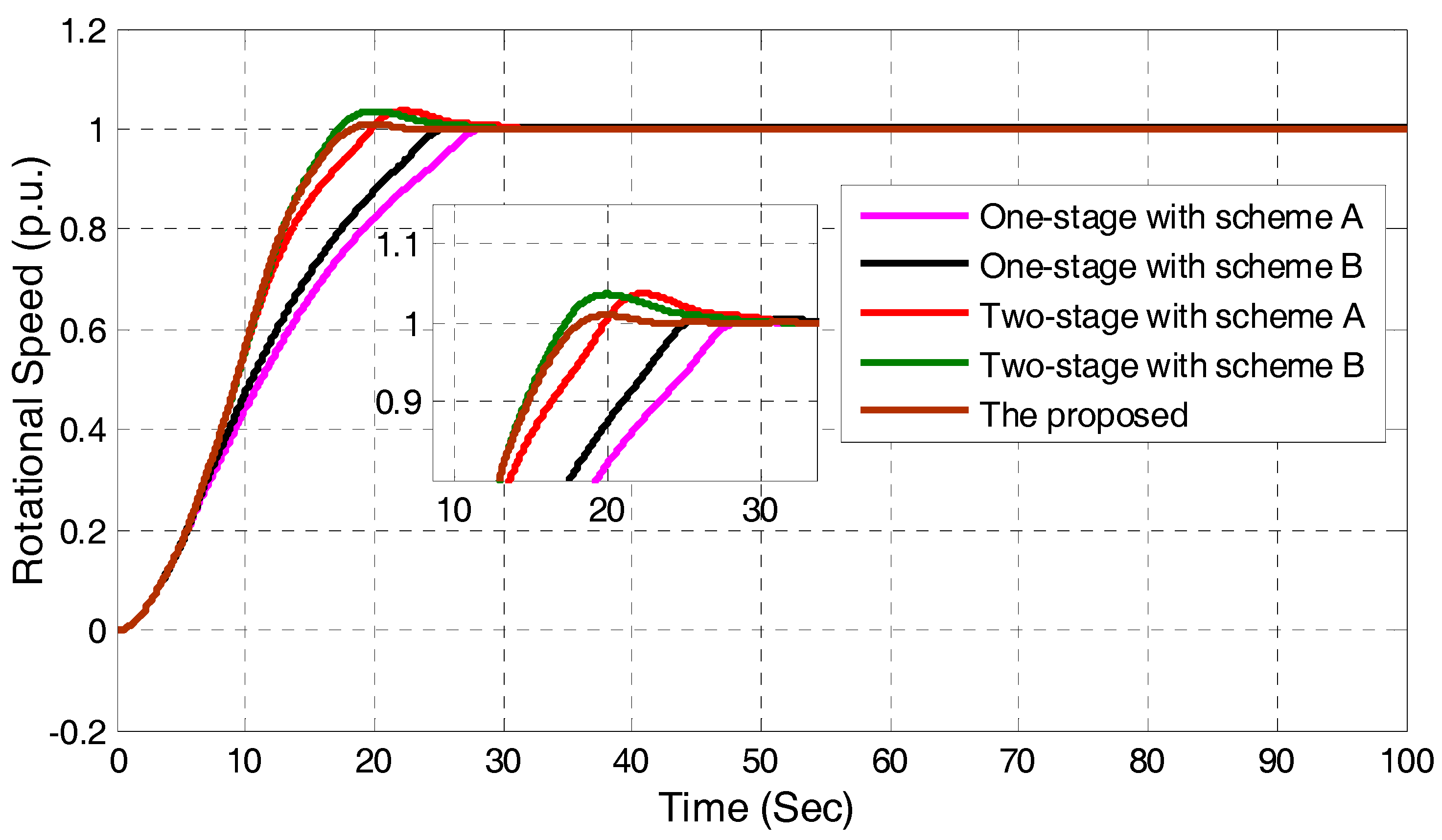
The results of different strategies are presented in Table 13 and Figure 20, where the indices of overshoot, start-up time and steady-state error are shown, and the rotational speed curves of start-up process are compared. From these results, it is easy to find out that the start-up time obtained by integrated start-up strategy is shorter than with other methods. This is especially important from the practical implementation point of view because it is a key index to evaluate the ability of quick connection to the grid. Because the guide vane opening is under closed-loop control in the whole start-up process, the control system has a better dynamic quality. Indices of overshoot and steady-state error obtained by the integrated method are still satisfactory, although the overshoot obtained by the integrated model is a little bigger than one-stage start-up strategy.
5.4. Performance under Different Initial Water Head Condition
In practical operation, the water head of a PSU might vary frequently. Hence other two initial conditions (T2 and T3) with different water levels in the upper and downstream reservoir have been adopted to test the performance of the discussed start-up methods. Three initial working conditions are listed in Table 14.
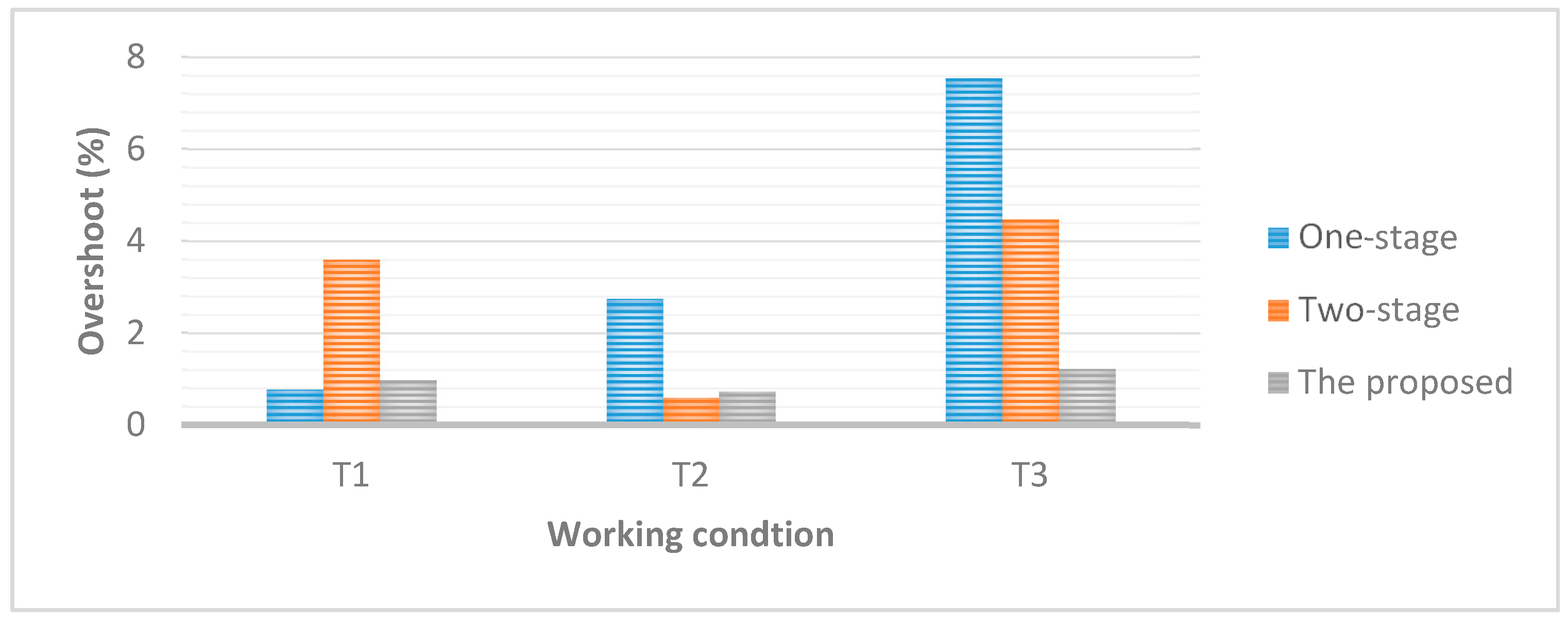
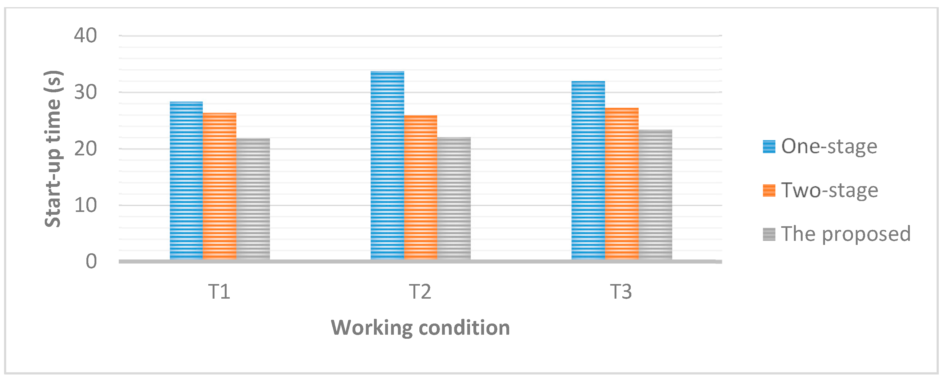
Traditional start-up strategies, including the one-stage strategy and two-stage strategy are optimized in Scheme B. The performance indices of different shut-up methods under various head conditions are presented in Table 15. Compared with the traditional start-up strategies, the proposed method has achieved the best performance on all indices overall. Especially, the start-up time has been significantly shortened by the proposed method under all working conditions.
In order to show the results more explicitly, bar graphs of the indices of overshoot and start-up time are exhibited in Figure 21 and Figure 22. From these figures, it’s clearly shown that a smooth and swift start-up of PSU could be realized by applying the proposed integrated start-up strategy, with an extremely low overshoot and a short start-up time. Compared with one-stage strategy, the proposed method has shortened the start-up time 22.8%, 34.4%, 26.9% under the three working conditions.
6. Conclusions
In order to improve the start-up process indices, a new integrated start-up method is proposed. In this method, a two-phase closed-loop start-up strategy is designed, while PI control is applied to quickly open the guide vane with a specially designed control target in the first phase, and PID control is adopted to adjust the rotational speed of a PSU to track the rated value in the second phase. What’s more, an integrated optimization method is used to synchronously tune the parameters of the PI and PID controllers.
To solve this complicated optimization problem, the ASA, a novel meta-heuristic that mimics the social behaviors of sheep, has been proposed and fully verified by comparing it with seven popular meta-heuristics on 13 typical benchmark functions. The results show that the ASA significantly outperforms all competitors for high dimension numerical functions.
Based on the mathematical model of PSUs, the control system, PTGS, has been modeled and simulated in MATLAB, and simulation experiments on different start-up strategies have been conducted. The proposed method has been compared with the traditional one-stage DGVC, and two-stage DGVC strategies with different optimization schemes. The experimental results have revealed that the proposed integrated start-up method shows great advantages in terms of performance indices, i.e., overshoot, start-up time, compared with the traditional start-up strategies. The start-up time could be improved by as much as 34%, while maintaining the overshoot under a low level. The significant improvements on these key indices is interesting and merit further application in real PSUs.
Acknowledgments
This paper is supported by the National Key Research and Development Program of China (2016YFC0401905) and the National Natural Science Foundation of China (No. 51679095, No. 51479076).
Author Contributions
C.L. and Y.X. conceived and designed the experiments; Z.W. and X.L. performed the simulations; N.Z. analyzed the data; Z.W. and J.H. wrote the paper; C.L. and Y.X. played an important role in the process of revising the paper.
Conflicts of Interest
The authors declare no conflict of interest.
Abbreviations
| PSU | Pumped Storage Unit |
| RE | Renewable Energy |
| DGVC | Direct Guide Vane Control |
| GVO | Guide Vane Opening |
| MOC | Method Of Characteristic |
| ITAE | Integral Time Absolute Error |
| PSO | Particle Swarm Optimization |
| ACO | Ant Colony Optimization |
| CS | Cuckoo Search |
| GSA | Gravitational Search Algorithm |
| PID | Proportional-Integral-Derivative |
| ASA | Artificial Sheep Algorithm |
| GV | Guide Vane |
| PTGS | Pump-Turbine Governing System |
| PDE | Partial Differential Equation |
| PSHP | Pumped Storage Hydropower Plant |
| DE | Differential Evolution |
| ABC | Artificial Bee Colony |
| GWO | Grey Wolf Optimizer |
| GA | Genetic Algorithm |
Nomenclature
| PTGS | |
| c | Velocity of pressure wave |
| D | Inner diameter of the pipe |
| f | Darcy-Weisbach coefficient of friction resistance |
| g | Gravitational acceleration |
| H | Piezometric water head in the pipeline |
| t | Time |
| V | Average flow velocity of pipeline section |
| L | Pipeline total length |
| Q | Water flow in the pipeline |
| a | The relative value of turbine speed |
| q | The relative value of turbine flow |
| h | The relative value of water head |
| m | The relative value of turbine torque |
| x | Horizontal coordinate of curves WH and WM |
| J | Moment of inertia |
| kc | The rising slope of guide vane |
| yc1 | The maximum value of GVO |
| fc | The set frequency |
| ts | Start-up time |
| A | Cross section area of pipeline |
| Ta | Inertia time constant of the generator |
| Nn | Turbine speed at time n |
| k0 | The gain coefficient of servo-mechanism |
| TyB | The assistant servomotor response time |
| Ty | The main servomotor response time |
| n | Time of simulation |
| Qn | Water flow at time n |
| Ca | Depends on the pipeline characteristics |
| Accuracy index for calculating Q | |
| Accuracy index for calculating N | |
| Iterative coefficient for calculating Q and N | |
| kmax | Maximum iterative number for calculating Q and N |
| N11 | Unit turbine speed |
| nc | A set value of turbine speed |
| yc | Maximum value of GVO |
| yc2 | The minimum value after guide vane close |
| amax | Relative value of the peak speed |
References
- Pan, I.; Das, S. Fractional order fuzzy control of hybrid power system with renewable generation using chaotic PSO. ISA Trans. 2016, 62, 19–29. [Google Scholar] [CrossRef] [PubMed]
- Serban, I.; Marinescu, C. Battery energy storage system for frequency support in microgrids and with enhanced control features for uninterruptible supply of local loads. Int. J. Electr. Power Energy Syst. 2014, 54, 432–441. [Google Scholar] [CrossRef]
- Daud, M.Z.; Mohamed, A.; Hannan, M.A. An improved control method of battery energy storage system for hourly dispatch of photovoltaic power sources. Energy Convers. Manag. 2013, 73, 256–270. [Google Scholar] [CrossRef]
- Nguyen, T.T.; Yoo, H.J.; Kim, H.M. A Flywheel Energy Storage System Based on a Doubly Fed Induction Machine and Battery for Microgrid Control. Energies 2015, 8, 5074–5089. [Google Scholar] [CrossRef]
- Wang, W.; Li, C.; Liao, X.; Qin, H. Study on unit commitment problem considering pumped storage and renewable energy via a novel binary artificial sheep algorithm. Appl. Energy 2017, 187, 612–626. [Google Scholar] [CrossRef]
- Ma, T.; Yang, H.; Lin, L.; Peng, J. Technical feasibility study on a standalone hybrid solar-wind system with pumped hydro storage for a remote island in Hong Kong. Renew. Energy 2014, 69, 7–15. [Google Scholar] [CrossRef]
- Yang, W.; Yang, J. Study on Optimum Start-Up Method for Hydroelectric Generating Unit Based on Analysis of the Energy Relation. In Proceedings of the Asia-Pacific Power and Energy Engineering Conference, Shanghai, China, 27–29 March 2012; pp. 1–5. [Google Scholar]
- Parastegari, M.; Hooshmand, R.A.; Khodabakhshian, A.; Zare, A.H. Joint operation of wind farm, photovoltaic, pump-storage and energy storage devices in energy and reserve markets. Int. J. Electr. Power Energy Syst. 2015, 64, 275–284. [Google Scholar] [CrossRef]
- Kocaman, A.S.; Modi, V. Value of pumped hydro storage in a hybrid energy generation and allocation system. Appl. Energy 2017, 205, 1202–1215. [Google Scholar] [CrossRef]
- Min, C.G.; Kim, M.K. Flexibility-Based Reserve Scheduling of Pumped Hydroelectric Energy Storage in Korea. Energies 2017, 10, 1478. [Google Scholar]
- Merino, J.; Veganzones, C.; Sanchez, J.A.; Martinez, S.; Platero, C.A. Power System Stability of a Small Sized Isolated Network Supplied by a Combined Wind-Pumped Storage Generation System: A Case Study in the Canary Islands. Energies 2012, 5, 2351–2369. [Google Scholar] [CrossRef] [Green Version]
- Saboya, I.; Egido, I.; Rouco, L. Start-Up Decision of a Rapid-Start Unit for AGC Based on Machine Learning. IEEE Trans. Power Syst. 2013, 28, 3834–3841. [Google Scholar] [CrossRef]
- Trivedi, C.; Cervantes, M.J.; Gandhi, B.K.; Ole Dahlhaug, G. Experimental investigations of transient pressure variations in a high head model Francis turbine during start-up and shutdown. J. Hydrodyn. Ser. B 2014, 26, 277–290. [Google Scholar] [CrossRef]
- Lindenmeyer, D.; Moshref, A.; Schaeffer, C.; Benge, A. Simulation of the start-up of a Hydro Power plant for the emergency power supply of a nuclear power station. IEEE Trans. Power Syst. 2001, 16, 163–169. [Google Scholar] [CrossRef]
- Ling, K.; Ye, L.; Jiang, T. A closed-loop start-up control strategy and its simulation studies for hydroelectric generating units. In Proceedings of the International Conferences on Info-Tech and Info-Net (ICII 2001), Beijing, China, 29 October–1 November 2001; Volume 4, pp. 209–214. [Google Scholar]
- Chen, S.Y.; Zhang, G.S.; Zhao, R.; Cao, N.; Cao, B.D. Program control based starting-up control strategy of hydroelectric generating sets. Power Syst. Technol. 2005, 29. [Google Scholar] [CrossRef]
- Bao, H.; Yang, J.; Fu, L. Study on Nonlinear Dynamical Model and Control Strategy of Transient Process in Hydropower Station with Francis Turbine. In Proceedings of the Power and Energy Engineering Conference (APPEEC 2009), Wuhan, China, 27–31 March 2009; pp. 1–6. [Google Scholar]
- Zhang, J.B.; Xie, J.C.; Jiao, S.B. Study on optimum start-up rule for hydroelectric generating units. J. Hydraul. Eng. 2004, 35, 53–59. [Google Scholar]
- Zhou, B.; Yongliang, S.U.; Luo, R.; Jin, W.U. Comparison and Optimization of Two Control Technologies on Hydraulic Turbine Start-up Process. Hydropower Autom. Dam Monit. 2013, 37. [Google Scholar] [CrossRef]
- Xu, Y.; Zhou, J.; Xue, X.; Fu, W.; Zhu, W.; Li, C. An adaptively fast fuzzy fractional order PID control for pumped storage hydro unit using improved gravitational search algorithm. Energy Convers. Manag. 2016, 111, 67–78. [Google Scholar] [CrossRef]
- Pannatier, Y.; Kawkabani, B.; Nicolet, C.; Schwery, A.; Simond, J.J. Optimization of the start-up time of a variable speed pump-turbine unit in pumping mode. In Proceedings of the XXth International Conference on Electrical Machines, Marseille, France, 2–5 September 2012; pp. 2126–2132. [Google Scholar]
- Li, C.; Chang, L.; Huang, Z.; Liu, Y.; Zhang, N. Parameter identification of a nonlinear model of hydraulic turbine governing system with an elastic water hammer based on a modified gravitational search algorithm. Eng. Appl. Artif. Intell. 2016, 50, 177–191. [Google Scholar] [CrossRef]
- Wang, Q.; Zhang, M.; Bai, D.; Yin, Y.; Hao, X. Fuzzy Adaptive PID Control for Multi-range Hydro-mechanical Continuously Variable Transmission in Tractor. J. Mech. Transm. 2016, 12. [Google Scholar]
- Goldberg, D.E. Genetic Algorithm in Search, Optimization, and Machine Learning; Addison-Wesley: Reading, UK, 1989. [Google Scholar]
- Kennedy, J.; Eberhart, R. Particle swarm optimization. In Proceedings of the IEEE International Conference on Neural Networks, Perth, WA, Australia, 27 November–1 December 1995. [Google Scholar]
- Dorigo, M.; Maniezzo, V.; Colorni, A. The Ant System: Optimization by a colony of cooperating agents. IEEE Trans. Syst. Man Cybern. 1996, 26, 29–41. [Google Scholar] [CrossRef] [PubMed]
- Rashedi, E.; Nezamabadi-Pour, H.; Saryazdi, S. GSA: A Gravitational Search Algorithm; Elsevier Science Inc.: Amsterdam, The Netherlands, 2009. [Google Scholar]
- Li, C.; Zhou, J.; Xiao, J.; Xiao, H. Hydraulic turbine governing system identification using T–S fuzzy model optimized by chaotic gravitational search algorithm. Eng. Appl. Artif. Intell. 2013, 26, 2073–2082. [Google Scholar] [CrossRef]
- Li, C.; Zhou, J. Semi-supervised weighted kernel clustering based on gravitational search for fault diagnosis. ISA Trans. 2014, 53, 1534–1543. [Google Scholar] [CrossRef] [PubMed]
- Li, C.; Mao, Y.; Yang, J.; Wang, Z.; Xu, Y. A nonlinear generalized predictive control for pumped storage unit. Renew. Energy 2017, 114, 945–959. [Google Scholar] [CrossRef]
- Zhou, J.; Xu, Y.; Zheng, Y.; Zhang, Y. Optimization of Guide Vane Closing Schemes of Pumped Storage Hydro Unit Using an Enhanced Multi-Objective Gravitational Search Algorithm. Energies 2017, 10, 911. [Google Scholar] [CrossRef]
- Popescu, M.; Arsenie, D.; Vlase, P. Applied Hydraulic Transients: For Hydropower Plants and Pumping Stations; CRC Press: Boca Raton, FL, USA, 2003. [Google Scholar]
- Sim, W.G.; Park, J.H. Transient analysis for compressible fluid flow in transmission line by the method of characteristics. KSME Int. J. 1997, 11, 173–185. [Google Scholar] [CrossRef]
- Chalghoum, I.; Elaoud, S.; Akrout, M.; Taieb, E.H. Transient behavior of a centrifugal pump during starting period. Appl. Acoust. 2016, 109, 82–89. [Google Scholar] [CrossRef]
- Zheng, X.B.; Guo, P.C.; Tong, H.Z.; Luo, X.Q. Improved Suter-transformation for complete characteristic curves of pump-turbine. In Proceedings of the IOP Conference Series: Earth and Environmental Science, Beijing, China, 19–23 August 2012; Volume 15. [Google Scholar]
- Liu, Z.M.; Zhang, D.H.; Liu, Y.Y.; Zhang, X. New Suter-transformation Method of Complete Characteristic Curves of Pump-turbines Based on the 3-D Surface. China Rural Water Hydropower 2015. [Google Scholar] [CrossRef]
- Li, C.; Zhang, N.; Lai, X.; Zhou, J.; Xu, Y. Design of a fractional-order PID controller for a pumped storage unit using a gravitational search algorithm based on the Cauchy and Gaussian mutation. Inf. Sci. 2017, 396, 162–181. [Google Scholar] [CrossRef]
- Chen, Z.; Yuan, Y.; Yuan, X.; Huang, Y.; Li, X.; Li, W. Application of multi-objective controller to optimal tuning of PID gains for a hydraulic turbine regulating system using adaptive grid particle swam optimization. ISA Trans. 2015, 56, 173–187. [Google Scholar] [CrossRef] [PubMed]
- Das, S.; Suganthan, P.N. Differential Evolution: A Survey of the State-of-the-Art. IEEE Trans. Evolut. Comput. 2011, 15, 4–31. [Google Scholar] [CrossRef]
- Guo, P.; Zhu, L. Ant colony optimization for continuous domains. Eur. J. Oper. Res. 2012, 185, 1155–1173. [Google Scholar]
- Karaboga, D.; Basturk, B. A powerful and efficient algorithm for numerical function optimization: Artificial bee colony (ABC) algorithm. J. Glob. Optim. 2007, 39, 459–471. [Google Scholar] [CrossRef]
- Yang, X.S.; Deb, S. Cuckoo Search via Lévy flights. In Proceedings of the World Congress on Nature & Biologically Inspired Computing (NaBIC 2009), Coimbatore, India, 9–11 December 2009; pp. 210–214. [Google Scholar]
- Mirjalili, S.; Mirjalili, S.M.; Lewis, A. Grey Wolf Optimizer. Adv. Eng. Softw. 2014, 69, 46–61. [Google Scholar] [CrossRef]
- El-Abd, M. Performance assessment of foraging algorithms vs. evolutionary algorithms. Inf. Sci. 2012, 182, 243–263. [Google Scholar] [CrossRef]
- Åström, K.J.; Hägglund, T. PID Controllers: Theory, Design and Tuning; Instrument Society of America Research: Triangle Park, NC, USA, 1995. [Google Scholar]
- Vilanova, R.; Visioli, A. PID Control in the Third Millennium; Springer: London, UK, 2012. [Google Scholar]
- Maiti, D.; Acharya, A.; Chakraborty, M.; Konar, A.; Janarthanan, R. Tuning PID and PI/λDδ Controllers using the Integral Time Absolute Error Criterion. In Proceedings of the International Conference on Information and Automation for Sustainability, Colombo, Sri Lanka, 12–14 December 2008. pp. 457–462.
Figure 1.
Structure of pumped storage unit governing system.
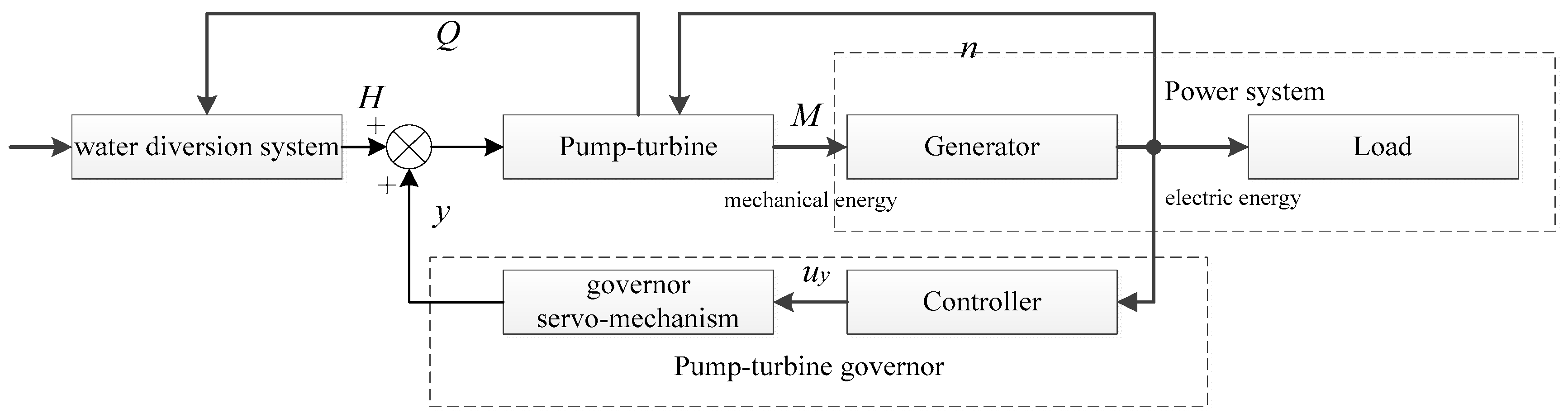
Figure 2.
Characteristic lines in L-t plane of MOC.
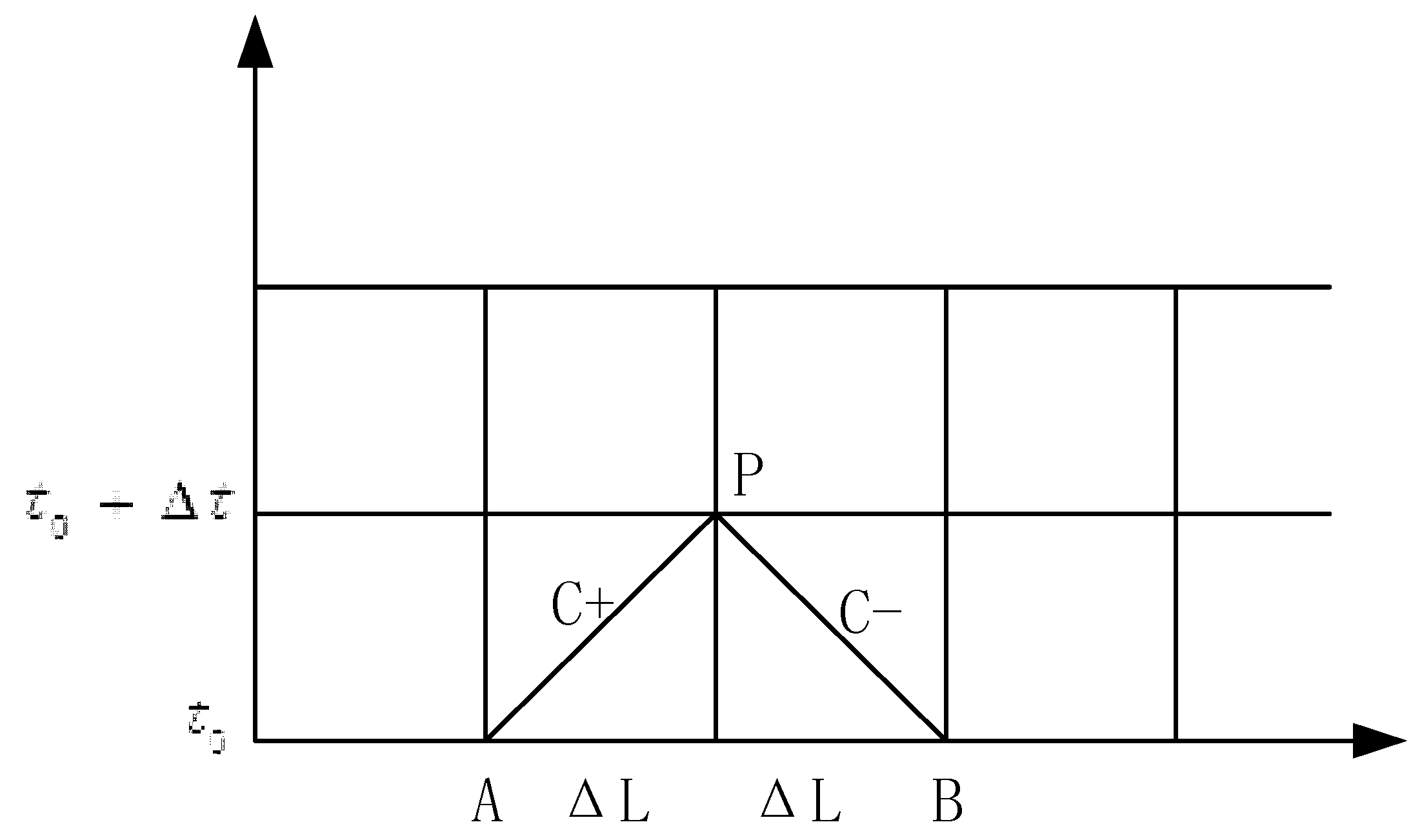
Figure 3.
Characteristic curve of a pump-turbine. (a) flow characteristic curve; and (b) torque characteristic curve.
Figure 3.
Characteristic curve of a pump-turbine. (a) flow characteristic curve; and (b) torque characteristic curve.
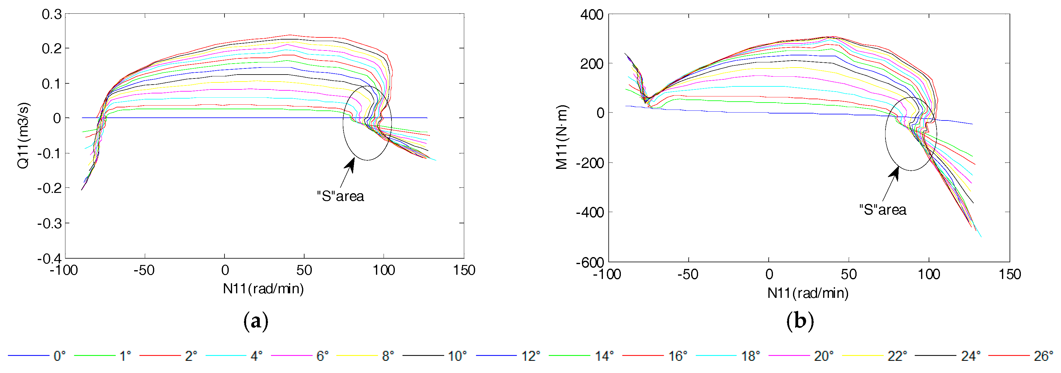
Figure 4.
The WH and WM curves transformed by the improved Suter transformation method.

Figure 5.
Structure of the servomechanism.

Figure 6.
The water flow and turbine speed calculation of the PTGS.
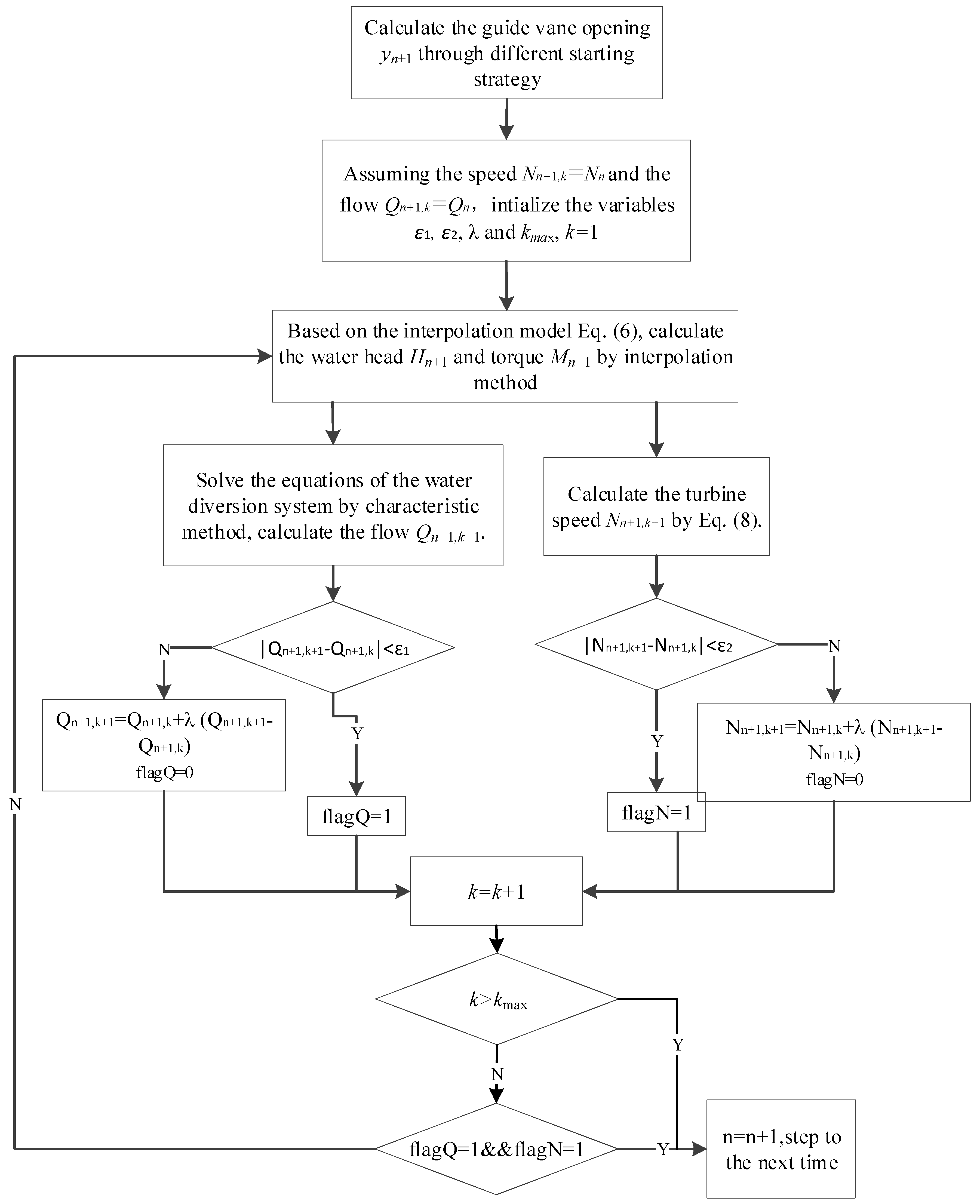
Figure 7.
Flowchart of ASA optimization.

Figure 8.
Comparison of performance of different algorithms for minimization of high dimensional unimodal functions. (a) unimodal test function F1; (b) unimodal test function F2; (c) unimodal test function F3; (d) unimodal test function F4; (e) unimodal test function F5; (f) unimodal test function F6 and (g) unimodal test function F7.
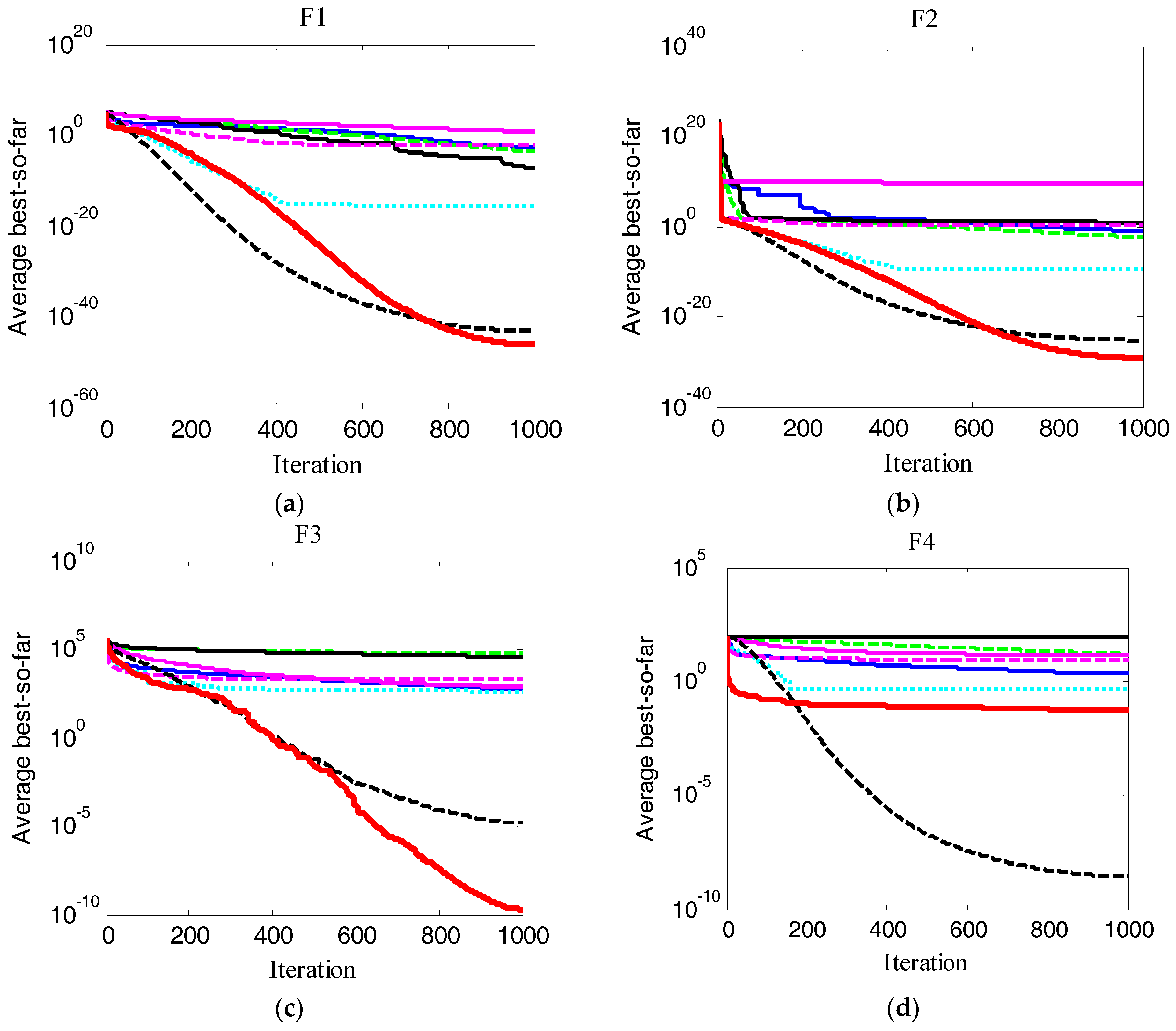

Figure 9.
Comparison of performance of different algorithms for minimization of high dimensional multimodal functions. (a) multimodal test function F8; (b) multimodal test function F9; (c) multimodal test function F10; (d) multimodal test function F11; (e) multimodal test function F12 and (f) multimodal test function F13.

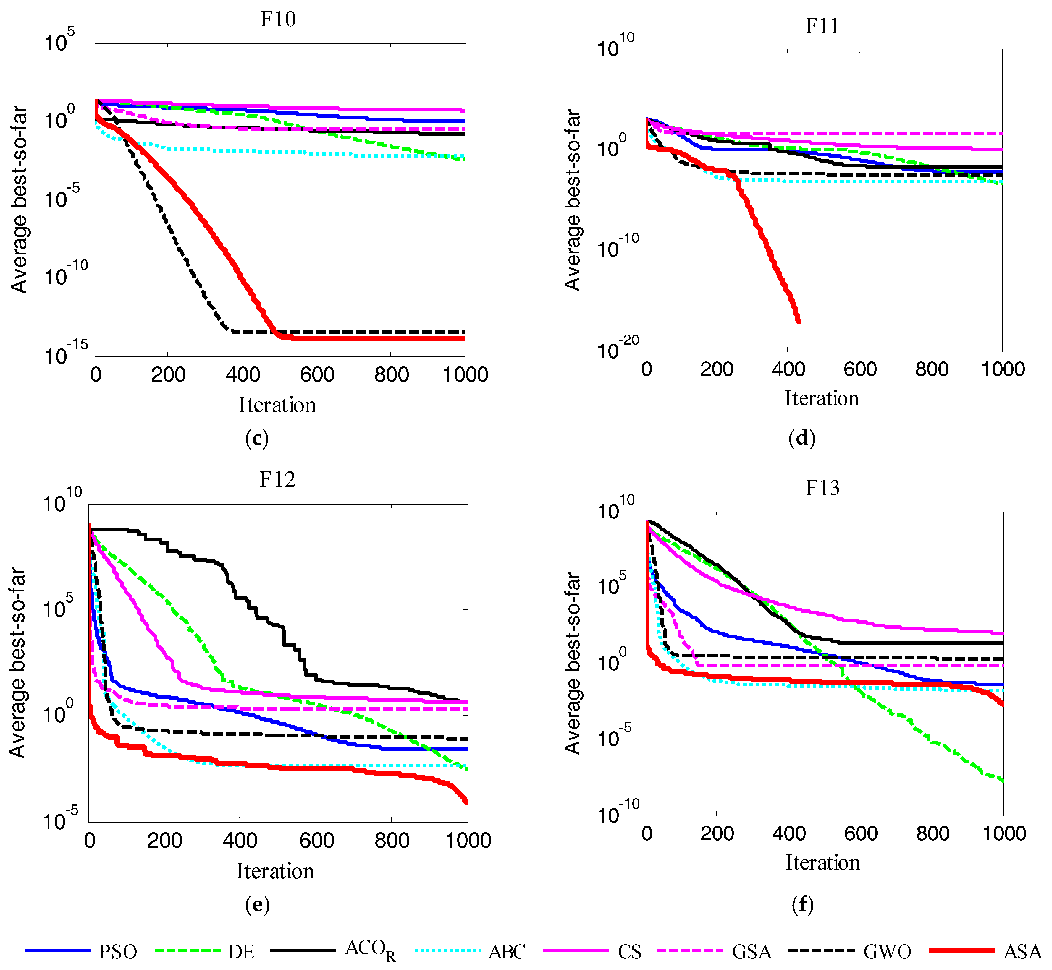
Figure 10.
One-stage DGVC law.
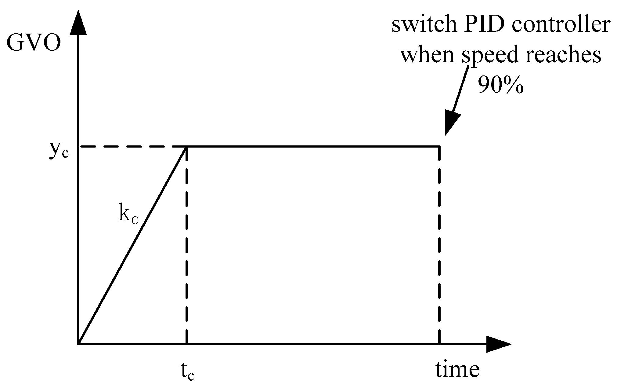
Figure 11.
Two-stage DGVC.

Figure 12.
The rotational speed speed curves of PSU.
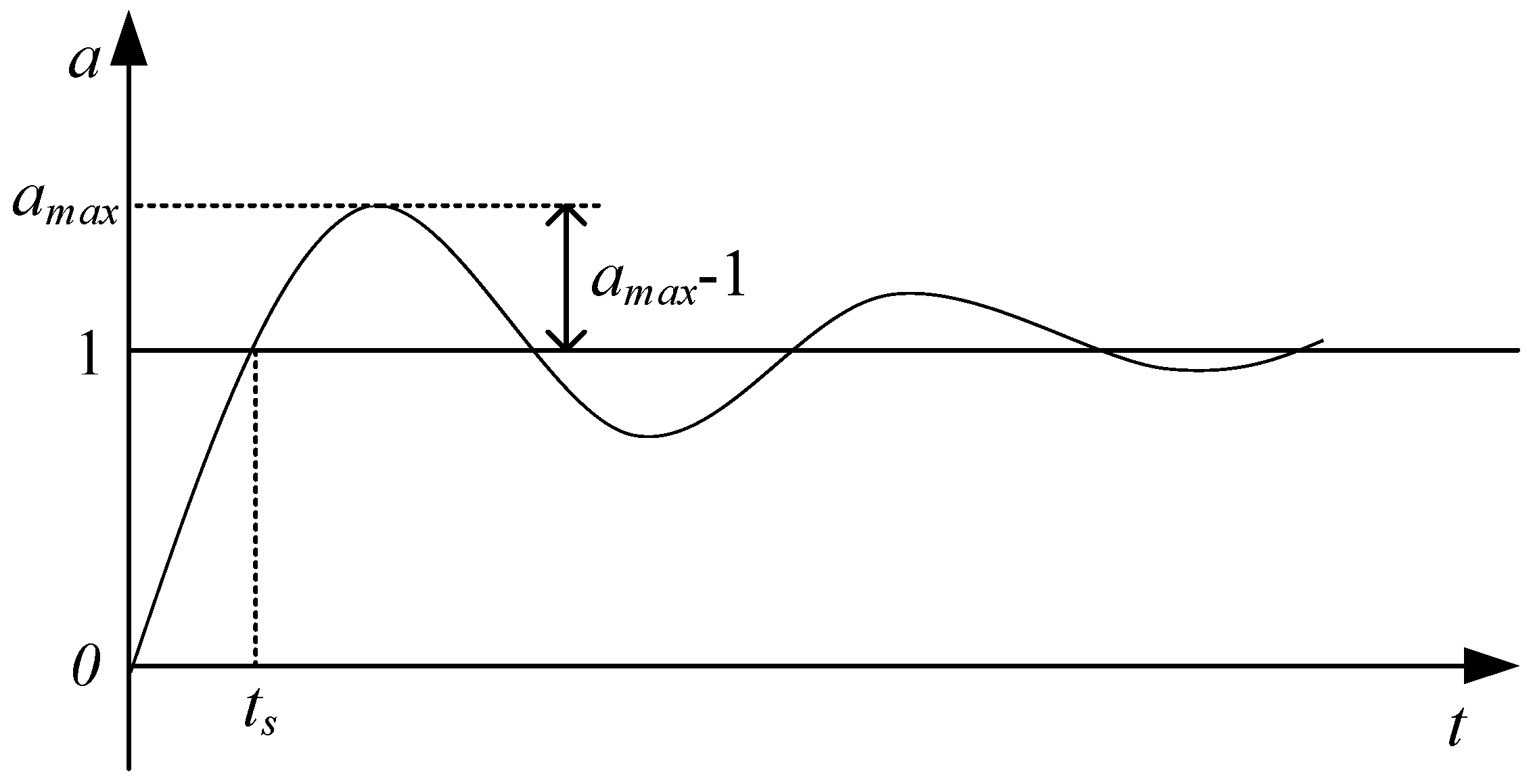
Figure 13.
The detail flow chart of parameters optimization.

Figure 14.
Structure of the water diversion system.

Figure 15.
Rotational speed of traditional start-up strategies with Scheme A.

Figure 16.
Change process of guide vane opening of traditional start-up strategies with Scheme A.

Figure 17.
Rotational speed of traditional start-up strategies with Scheme B.

Figure 18.
Change process of guide vane opening of traditional start-up strategies with Scheme B.
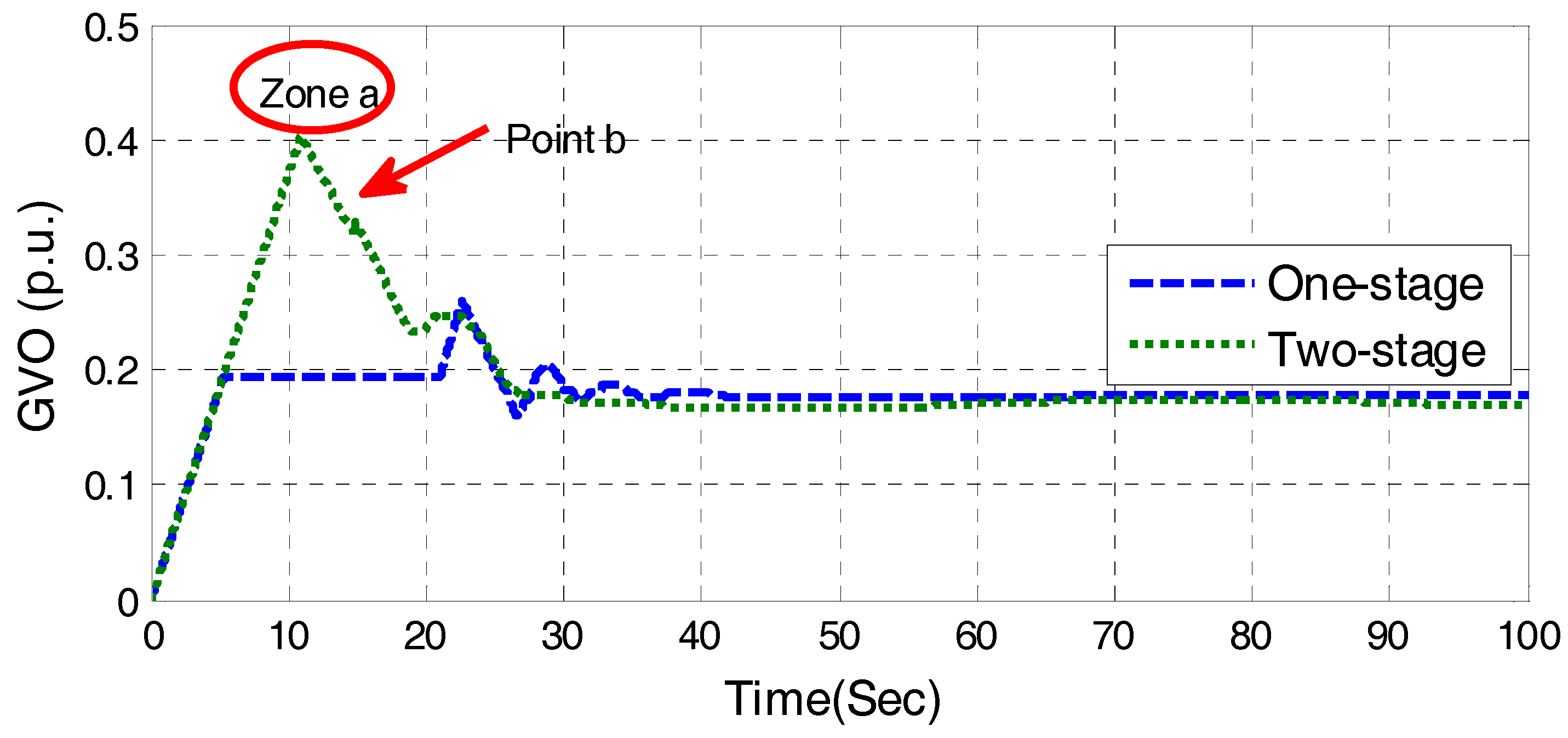
Figure 19.
Comprehensive results of integrated start-up strategy.

Figure 20.
Comparison of rotational speed of each start-up strategy.

Figure 21.
Index of overshoot under different working conditions.

Figure 22.
Index of start-up time under different working conditions.


Table 1.
Unimodal test functions (D = 50).
| Test Function | Range |
|---|---|
| [−100, 100]D | |
| [−10, 10]D | |
| [−100, 100]D | |
| [−100, 100]D | |
| [−30, 30]D | |
| [−100, 100]D | |
| [−1.28, 1.28]D |
Table 2.
Multimodal test function (D = 50).
| Test Function | Range |
|---|---|
| [−500, 500]D | |
| [−5.12, 5.12]D | |
| [−32, 32]D | |
| [−600, 600]D | |
| [−50, 50]D | |
| [−50, 50]D |
Table 3.
Mean, best and standard deviation values of solutions achieved for unimodal test functions taken over 30 runs.
Table 3.
Mean, best and standard deviation values of solutions achieved for unimodal test functions taken over 30 runs.
| PSO | DE | ACOR | ABC | CS | GSA | GWO | ASA | ||
|---|---|---|---|---|---|---|---|---|---|
| F1 | Best | 2.59 × 10⁻⁵ | 0.000125 | 6.78 × 10⁻¹⁰ | 5.40 × 10⁻¹⁹ | 2.545205 | 2.21 × 10⁻¹⁵ | 2.80 × 10−45 | 4.00 × 10−47 |
| Mean | 0.003453 | 0.000283 | 6.37 × 10⁻⁸ | 1.57 × 10⁻¹⁶ | 6.777254 | 0.007024 | 8.64 × 10−44 | 6.31 × 10−42 | |
| Std | 0.01392 | 0.000118 | 1.37 × 10⁻⁷ | 2.99 × 10⁻¹⁶ | 2.588802 | 0.02132 | 1.39 × 10−43 | 3.17 × 10−41 | |
| F2 | Best | 0.023024 | 0.002001 | 2.71 × 10⁻⁶ | 1.76 × 10⁻¹² | 5.076218 | 3.39 × 10⁻⁷ | 6.12 × 10⁻²⁷ | 9.81 × 10⁻³¹ |
| Mean | 0.12412 | 0.004183 | 6.000077 | 2.21 × 10⁻¹⁰ | 3 × 10⁹ | 1.052277 | 5.16 × 10⁻²⁶ | 3.49 × 10⁻²⁸ | |
| Std | 0.160725 | 0.001342 | 7.70134 | 2.80 × 10⁻¹⁰ | 4.66 × 10⁹ | 1.819242 | 4.44 × 10⁻²⁶ | 6.62 × 10⁻²⁸ | |
| F3 | Best | 230.6381 | 48344.53 | 24835.99 | 7.992538 | 251.9153 | 1035.82 | 4.51 × 10⁻¹¹ | 1.36 × 10⁻¹⁶ |
| Mean | 556.8782 | 61553.98 | 38502.07 | 316.2684 | 751.5542 | 2121.014 | 1.53 × 10⁻⁵ | 4.95 × 10⁻⁸ | |
| Std | 178.079 | 6337.879 | 7592.073 | 277.9050 | 282.7432 | 566.2951 | 7.19 × 10⁻⁵ | 2.66 × 10⁻⁷ | |
| F4 | Best | 1.820148 | 12.32438 | 87.49964 | 0.036120 | 9.132951 | 4.172456 | 8.46 × 10⁻¹¹ | 0.000178 |
| Mean | 2.249488 | 15.60988 | 92.4693 | 0.411885 | 14.91595 | 9.381604 | 2.67 × 10⁻⁹ | 0.035010 | |
| Std | 0.283119 | 2.545444 | 2.144256 | 0.270970 | 2.481156 | 1.901231 | 3.13 × 10⁻⁹ | 0.025305 | |
| F5 | Best | 50.08615 | 48.63219 | 22.10962 | 24.10442 | 439.6469 | 83.36688 | 45.31071 | 0.00026 |
| Mean | 281.4765 | 61.03248 | 316.0433 | 25.02321 | 1328.587 | 267.8605 | 47.11051 | 0.796821 | |
| Std | 358.3448 | 3.73 × 101 | 758.5534 | 0.368753 | 866.8021 | 192.4422 | 0.837187 | 1.043769 | |
| F6 | Best | 5.76 × 10⁻⁵ | 0.000118 | 2.05 × 10⁻⁹ | 3.15 × 10⁻⁷ | 29 | 5.76 × 10⁻¹⁵ | 1.505454 | 1.02 × 10⁻⁶ |
| Mean | 0.001352 | 0.000306 | 2.01 × 10⁻⁶ | 5.12 × 10⁻⁶ | 60.43333 | 0.003991 | 2.463479 | 0.146174 | |
| Std | 0.002104 | 0.000117 | 1.06 × 10⁻⁵ | 5.92 × 10⁻⁶ | 21.66625 | 0.020979 | 0.532694 | 0.737852 | |
| F7 | Best | 0.223833 | 0.164606 | 21.12714 | 8.325989 | 0.113516 | 0.231023 | 0.000248 | 1.19 × 10⁻⁵ |
| Mean | 0.446835 | 0.258014 | 23.26484 | 9.56142 | 0.237656 | 1.383992 | 0.001543 | 0.001756 | |
| Std | 0.153217 | 0.033662 | 1.529113 | 0.49641 | 0.08223 | 2.041238 | 0.000938 | 0.001532 |
Table 4.
Mean, best and standard deviation values of solutions achieved for multimodal test functions taken over 30 runs.
Table 4.
Mean, best and standard deviation values of solutions achieved for multimodal test functions taken over 30 runs.
| PSO | DE | ACOR | ABC | CS | GSA | GWO | ASA | ||
|---|---|---|---|---|---|---|---|---|---|
| F8 | Best | −4712.89 | −10238.1 | −16992.1 | −11535.6 | −13521.4 | −5076.05 | −10857.1 | −20949.1 |
| Mean | −2796.73 | −8966.34 | −14809.9 | −10795.1 | −12888.8 | −3360.46 | −9346.87 | −20949.1 | |
| Std | 791.2755 | 472.7152 | 649.162 | 465.5335 | 305.9319 | 646.0058 | 838.7516 | 0.026194 | |
| F9 | Best | 93.19619 | 278.5933 | 97.38696 | 0 | 92.36084 | 44.77313 | 0 | 0 |
| Mean | 132.2983 | 322.4454 | 223.8093 | 5.146369 | 132.2034 | 77.02013 | 0.240699 | 0 | |
| Std | 26.68086 | 15.32829 | 111.5528 | 6.148586 | 19.80883 | 19.80864 | 1.143943 | 0 | |
| F10 | Best | 0.008998 | 0.001541 | 0.011792 | 0.000396 | 2.761509 | 2.65 × 10⁻⁸ | 2.58 × 10⁻¹⁴ | 7.99 × 10⁻¹⁵ |
| Mean | 0.962793 | 0.003375 | 0.131553 | 0.005502 | 4.817019 | 0.295493 | 3.19 × 10⁻¹⁴ | 1.70 × 10⁻¹⁴ | |
| Std | 0.666548 | 0.000738 | 0.140057 | 0.004212 | 0.962438 | 0.457241 | 3.22 × 10⁻¹⁵ | 4.14 × 10⁻¹⁵ | |
| F11 | Best | 4.04 × 10⁻⁶ | 0.000146 | 7.37 × 10⁻¹⁰ | 0 | 1.008131 | 17.99741 | 0 | 0 |
| Mean | 0.005948 | 0.000392 | 0.017358 | 0.000575 | 1.06668 | 31.3846 | 0.002693 | 0 | |
| Std | 0.008839 | 0.000222 | 0.028997 | 0.002212 | 0.037663 | 6.600331 | 0.00555 | 0 | |
| F12 | Best | 5.21 × 10⁻⁷ | 0.000422 | 0.525900 | 1.84 × 10⁻⁵ | 2.360578 | 0.678241 | 0.034809 | 6.85 × 10⁻⁷ |
| Mean | 0.024906 | 0.002805 | 4.271751 | 0.004343 | 4.412597 | 2.315895 | 0.087145 | 6.61 × 10⁻⁵ | |
| Std | 0.053181 | 0.003206 | 1.400772 | 0.015570 | 1.719829 | 0.805198 | 0.034141 | 5.33 × 10⁻⁵ | |
| F13 | Best | 1.28 × 10⁻⁵ | 4.25 × 10⁻¹¹ | 8.636222 | 1.90 × 10⁻⁷ | 27.7498 | 2.21 × 10⁻³¹ | 1.15723 | 3.16 × 10⁻⁵ |
| Mean | 0.041362 | 1.99 × 10⁻⁸ | 19.01885 | 0.015484 | 94.52199 | 0.643825 | 1.870492 | 0 | |
| Std | 0.162455 | 7.63 × 10⁻⁸ | 7.79599 | 0.031675 | 187.1737 | 1.593794 | 0.333347 | 0 |
Note: In MATLAB, 2.2251 × 10−308 is the minimal real number, and the value “0” represent a small value smaller than 2.2251 × 10−308.
Table 5.
Parameters of the simulated model of PTGS.
| Components | Value | |||
|---|---|---|---|---|
| Suter transformation | k1 = 10 | k2 = 0.9 | Cy = 0.2 | Ch = 0.5 |
| Generator | J = 96.84 | |||
| Servo-mechanism | TyB = 0.05 | Ty = 0.3 | k0 = 1 | |
| Simulation setting | kmax = 20 | ts = 0.02 s |
Table 6.
The boundaries of each optimized parameter.
| Parameters | Boundary | Value | |||||
|---|---|---|---|---|---|---|---|
| BL | 0 | 0 | 0 | ||||
| BU | 10 | 5 | 10 | ||||
| BL | 0.1 | 0 | |||||
| BU | 0.4 | 1/27 | |||||
| BL | 0.3 | 0.1 | 0.4 | ||||
| BU | 0.8 | 0.3 | 0.9 | ||||
| BL | 0 | 0 | 0.01 | 0 | 0 | 0 | |
| BU | 20 | 20 | 1 | 10 | 5 | 10 | |
Table 7.
DGVC parameters selected by experience.
| Start-Up Strategy | Parameters | ||
|---|---|---|---|
| One-stage | yc = 0.167 | kc = 1/27 | |
| Two-stage | yc1 = 0.334 | yc2 = 0.167 | fc = 0.6 |
Table 8.
Optimized PID parameters in optimization Scheme A.
| Start-Up Strategy | Kp | Ki | Kd |
|---|---|---|---|
| One-stage | 5.35 | 0.04 | 9.97 |
| Two-stage | 4.064 | 1.509 | 9.90 |
Table 9.
Performance indices of traditional start-up strategy of PSU in optimization Scheme A.
| Start-Up Strategy | Performance Measure of Rotational Speed | ||
|---|---|---|---|
| IOvershoot (%) | Start-Up Time (s) | ISteady-state error (%) | |
| One-stage | 0.30 | 31.1 | 0.02 |
| Two-stage | 3.66 | 30.16 | 0.02 |
Table 10.
Optimized DGVC parameters in optimization Scheme B.
| Start-Up Strategy | Parameters | ||
|---|---|---|---|
| One-stage | yc = 0.193 | kc = 0.0368 | |
| Two-stage | yc1 = 0.413 | yc2 = 0.255 | fc = 0.64 |
Table 11.
Performance indices of traditional start-up strategy of PSU in optimization Scheme B.
| Scheme | Start-Up Strategy | Performance Measure of Rotational Speed | ||
|---|---|---|---|---|
| IOvershoot (%) | Start-Up Time (s) | ISteady-state error (%) | ||
| B | One-stage | 0.77 | 28.4 | 0.3 |
| Two-stage | 3.61 | 26.42 | 0.03 | |
Table 12.
Optimized parameters for integrated star-up method.
| Parameters | |||||
|---|---|---|---|---|---|
| Kp1 = 0.95 | Ki1 = 4.77 | C = 0.308 | Kp = 8.48 | Ki = 4.25 | Kd = 9.98 |
Table 13.
Performance indices of the variable start-up strategy of PSU with different scheme.
| Start-Up Strategy | Optimization Scheme | Performance Measure of Rotational Speed | ||
|---|---|---|---|---|
| IOvershoot (%) | Start-Up Time (s) | ISteady-state error (%) | ||
| One-stage | A | 0.3 | 31.1 | 0.02 |
| B | 0.77 | 28.4 | 0.3 | |
| Two-stage | A | 3.66 | 30.16 | 0.02 |
| B | 3.61 | 26.42 | 0.03 | |
| Integrated | - | 0.97 | 21.92 | 0.02 |
Table 14.
Working conditions.
| Condition Number | Upper Reservoir | Downstream Reservoir |
|---|---|---|
| T1 | 735.45 m | 181 m |
| T2 | 716 m | 181 m |
| T3 | 735.45 m | 189 m |
Table 15.
Performance indices of the variable start-up strategy of PSU under different water head conditions.
Table 15.
Performance indices of the variable start-up strategy of PSU under different water head conditions.
| Condition Number | Strategy | Performance Measure of Rotational Speed | ||
|---|---|---|---|---|
| IOvershoot (%) | Start-Up Time (s) | ISteady-state error (%) | ||
| T1 | One-stage | 0.77 | 28.4 | 0.3 |
| Two-stage | 3.61 | 26.42 | 0.03 | |
| Integrated | 0.97 | 21.92 | 0.02 | |
| T2 | One-stage | 2.75 | 33.76 | 0.9 |
| Two-stage | 0.59 | 25.94 | 0. 07 | |
| Integrated | 0.73 | 22.14 | 0.01 | |
| T3 | One-stage | 7.55 | 32.06 | 0.06 |
| Two-stage | 4.47 | 27.3 | 0.04 | |
| Integrated | 1.23 | 23.44 | 0.02 | |
© 2018 by the authors. Licensee MDPI, Basel, Switzerland. This article is an open access article distributed under the terms and conditions of the Creative Commons Attribution (CC BY) license (http://creativecommons.org/licenses/by/4.0/).
Share and Cite
MDPI and ACS Style
Wang, Z.; Li, C.; Lai, X.; Zhang, N.; Xu, Y.; Hou, J. An Integrated Start-Up Method for Pumped Storage Units Based on a Novel Artificial Sheep Algorithm. Energies 2018, 11, 151. https://doi.org/10.3390/en11010151
AMA Style
Wang Z, Li C, Lai X, Zhang N, Xu Y, Hou J. An Integrated Start-Up Method for Pumped Storage Units Based on a Novel Artificial Sheep Algorithm. Energies. 2018; 11(1):151. https://doi.org/10.3390/en11010151
Chicago/Turabian StyleWang, Zanbin, Chaoshun Li, Xinjie Lai, Nan Zhang, Yanhe Xu, and Jinjiao Hou. 2018. "An Integrated Start-Up Method for Pumped Storage Units Based on a Novel Artificial Sheep Algorithm" Energies 11, no. 1: 151. https://doi.org/10.3390/en11010151
Note that from the first issue of 2016, this journal uses article numbers instead of page numbers. See further details here.