A Grey-Box Dynamic Model of Plate Heat Exchangers Used in an Urban Heating System

Abstract

This paper deals with the establishment of a grey-box model of plate heat exchangers. First, a second-order state space model of plate heat exchangers is developed. Then, the model is solved by the white-box method and grey-box method, respectively. In the white-box method, the linearization of the state space model is carried out by implicit difference scheme and the overall heat transfer coefficient was calculated with empirical correlation of the Nusselt number. In the grey-box method, a newly developed parameter identification method was established. The simulation results of two outlet temperatures by the grey-box and white-box method, respectively, are compared with the test data. It is shown that the grey-box method is more suitable and accurate for the simulations of outlet temperatures than the white-box method. Thus, it can provide practitioners and heating engineers with tools to design controllers for district heating systems.

1. Introduction

Heat exchangers are commonly used in many fields such as power, district heating, heat recovery, industrial process cooling and heating, hydraulic oil cooling or cooling of machine tools. Plate heat exchangers (PHEs) are probably the most common type of heat exchangers due to their high heat transfer coefficients, compactness, convenience for cleaning, and flexibility.

Due to the importance of PHEs, many researchers have investigated modeling and the optimum design parameters for the system. In Gut and Pinto’s work [1], a mathematical model was developed in an algorithmic form for the steady-state simulation of gasketed PHEs with generalized configurations. The configuration influence on the exchanger performance was studied and a method for configuration optimization was developed. Gut et al. [2] presented a parameter estimation procedure for PHEs that handles experimental data from multiple configurations. The heat transfer correlations obtained for PHEs are intimately associated with the configurations experimentally tested and the corresponding flow distribution patterns. Gut and Pinto [3] proposed a screening method to find the optimal set of configurations of a given PHE. Mota et al. [4] proposed an algorithm based on the screening method, for the optimization of heat exchange area of PHEs. In the work of Zhang et al. [5], a general three-dimensional distributed parameter model (DPM) was developed for optimal design of the plate-fin heat exchanger. A three-dimensional (3D) numerical model of the plate-type heat exchanger was established, and the flow pattern and heat transfer effect of the cold and hot fluids were analyzed by using ANSYS (ANSYS, Inc., Canonsburg, PA, USA) [6]. It can effectively solve the problems of optimization design of a plate-type heat exchanger. Yang et al. [7] proposed a mathematical model to quantitatively evaluate the effect of flow maldistribution in a multi-channel heat exchanger by computational fluid dynamics (CFD) technology.

In district heating system, PHEs and their networks frequently undergo transients resulting from heat load variations and regulations. Consequently, it is very important to know the behavior of PHEs when they are subjected to transient flow.

Luo et al. [8] have developed a new linearized one-dimensional model to solve non-linear problems with small non-linear disturbances. Dwivedi and Das [9] presented a predictive model to suggest the transient response of PHEs, subjected to a step flow variation. They indicated that the theoretical model developed for flow transient is capable of predicting the transient performance of the PHEs satisfactorily. Laszczyk [10] proposed a simplified cross-convection model for a wide class of heat exchangers. The simplified tuning procedure of the model was suggested and verified based on experimental data. The validation results show that the suggested modeling and tuning method is useful for practical applications. In Turhan et al.’s work [11], a data-driven grey-box identification approach provided the physically meaningful nonlinear continuous-time model. The validated results by the Monte Carlo tool serve to demonstrate the effectiveness and the viable application of the suggested control solutions to air conditioning systems.

In the general case, the convective heat transfer coefficient was calculated with empirical correlations of the Nusselt number in the above literature. The Nusselt number is a function of the Reynolds number and the Prandtl number. The influence of the Reynolds and the Prandtl numbers on heat transfer in a wide range of their values cannot be accounted for by simple power equations with a constant using the Prandtl number exponent, which is usually used in empirical correlations. For this reason, a semi-empirical equation was proposed and the Prandtl number’s influence on heat transfer was discussed in [12].

In addition to the convective heat transfer coefficient, fouling resistance also impacts the overall heat transfer coefficient of PHE. Fouling of PHE leads to a rise in pressure drop across the exchanger and the decrease of the overall heat transfer coefficient. Jonsson et al. [13] proposed a method which used nonlinear physical state space model for detection of the fouling of heat exchangers in transient states. The model parameters were estimated by using an extended Kalman filter and measurements of inlet and outlet temperatures and mass flow rates. Mahdi et al. [14] proposed a two-dimensional dynamic model for milk fouling in a PHE and stated that the aggregation rate of unfolded protein is found to increase exponentially with wall temperatures rising and can be accompanied by a substantial reduction in the heat-transfer coefficient. Grijspeerdt et al. [15] carried out two-dimensional (2D) and 3D CFD simulations of flow between two corrugated plates to investigate the flow distribution for milk processing with respect to fouling.

Optimal operation and real-time control require a more accurate description of the time-domain behavior of heat exchangers. Therefore, it is necessary to develop a mathematical model of a PHE, which is easy to parameterize and accurate enough to capture the essential dynamics and nonlinearities. A simplified and efficient grey-box method is established in this paper, which can avoid the calculation of the overall heat transfer coefficient.

2. Modeling of Plate Heat Exchanger

In order to derive the mathematical model of the PHE, the following assumptions are considered.

(1)

The fluid is assumed to be incompressible.

(2)

Due to the short width of the heat transfer channels, the flow rate component perpendicular to the flow direction of the plate approximates to 0, and the temperature distribution in this direction is neglected.

(3)

Heat loss to the surroundings is ignored.

(4)

The fluid velocity in the main flow direction is high enough to justify that heat conduction along the flow direction can be neglected as compared to heat convection.

(5)

No phase change of the fluid occurs inside the heat exchanger.

(6)

The end effects of the first and last channels are neglected.

(7)

The thermal capacity of the plates is neglected.

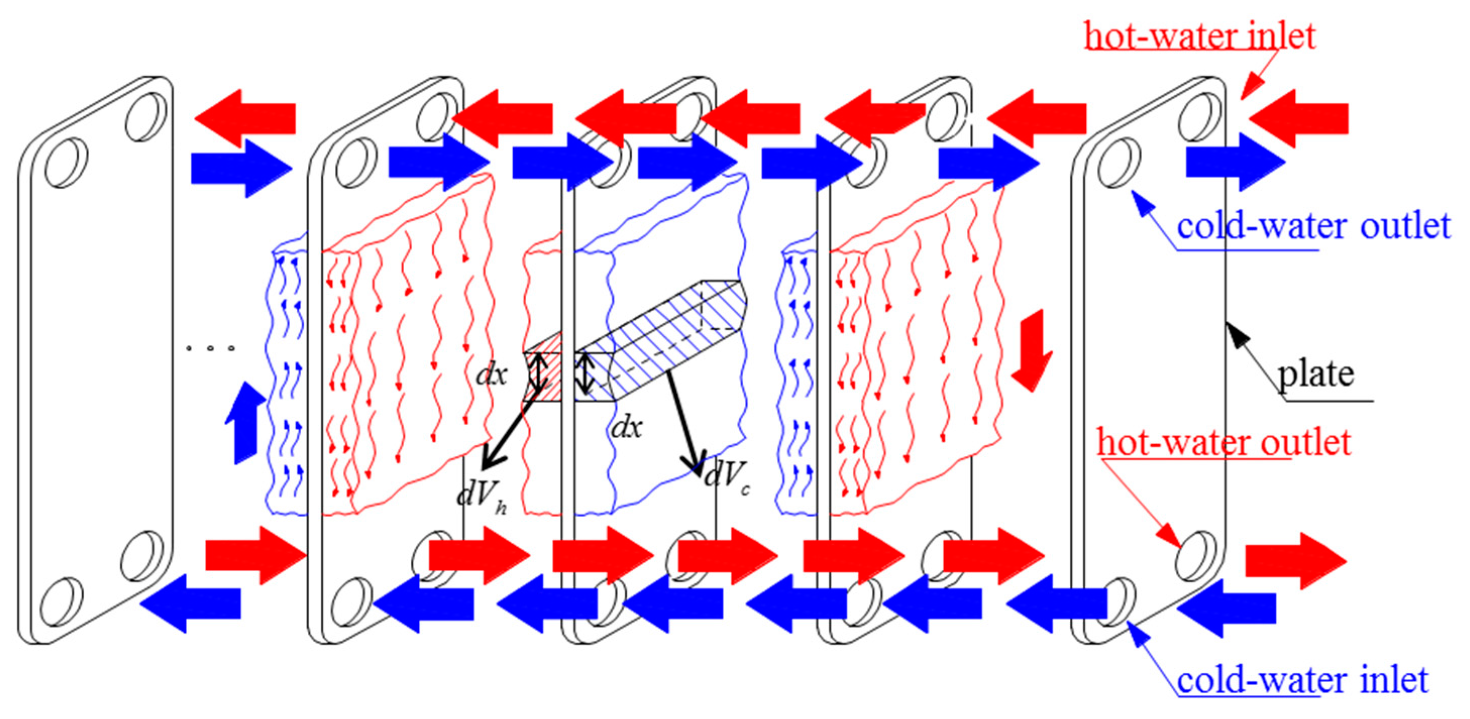
The fluid inside a channel exchanges heat with the neighbor channels through the plates, as shown in Figure 1. The arrangement of flow channels in each side is parallel. According to Assumption (2), the temperatures of cold and hot fluid in their respective channels are constant over the cross-section of channels. The control volumes $d{V}_h$ (in the hot water channel) and $d{V}_c$ (in the cold water channel) are shown in Figure 1, where,

$$d{V}_h=d{V}_c=\frac{{\delta }_p}{2}{b}_{p}dx$$

Applying the thermal balance to the control volumes shown in Figure 1, it is possible to derive the partial differential equations for the channel temperatures $T_h$ and $T_c$.

$${\rho }_w{c}_p\frac{{\delta }_p}{2}{b}_{p}dx\frac{\partial T_h}{\partial t}={\rho }_w{c}_p\frac{{\delta }_p}{2}{b}_p\left(T_h+\frac{\partial T_h}{\partial x}\frac{dx}{2}\right)u_h-{\rho }_w{c}_p\frac{{\delta }_p}{2}{b}_p\left(T_h-\frac{\partial T_h}{\partial x}\frac{dx}{2}\right)u_h+k{b}_{p}dx\left(T_c-T_h\right)$$

(1)

$${\rho }_w{c}_p\frac{{\delta }_p}{2}{b}_{p}dx\frac{\partial T_c}{\partial t}={\rho }_w{c}_p\frac{{\delta }_p}{2}{b}_p\left(T_c-\frac{\partial T_c}{\partial x}\frac{dx}{2}\right)u_c-{\rho }_w{c}_p\frac{{\delta }_p}{2}{b}_p\left(T_c+\frac{\partial T_c}{\partial x}\frac{dx}{2}\right)u_c+k{b}_{p}dx\left(T_h-T_c\right)$$

(2)

where ${\rho }_w$ is the fluid density (kg/m³); $c_p$ is specific heat (J/(kg·K)); ${\delta }_p$ is the distance between two neighboring plates (m); $b_p$ is the effective channel width which is obtained with the effective plate exchange area dividing by the length of the flow channel (m); $k$ denotes the overall heat transfer coefficient between the hot and cold fluid (W/(m²·K)); $T_c$ and $T_h$ are respectively the channel temperatures of cold and hot fluid (K); and $u_c$ and $u_h$ are the flow velocity of cold and hot fluid (m/s), respectively. Equations (1) and (2) can be simplified as:

$$\frac{\partial T_h}{\partial t}=u_h\frac{\partial T_h}{\partial x}+\frac{2k}{{\rho }_w{c}_p{\delta }_p}\left(T_c-T_h\right)$$

(3)

$$\frac{\partial T_c}{\partial t}=-u_c\frac{\partial T_c}{\partial x}+\frac{2k}{{\rho }_w{c}_p{\delta }_p}\left(T_h-T_c\right)$$

(4)

The overall heat transfer coefficient $k$ is obtained from Equation (5), which represents a series association of thermal resistances.

$$\frac{1}{k}=\frac{1}{h_h}+\frac{H_p}{{\lambda }_p}+\frac{1}{h_c}+R_{f,h}+R_{f,c}$$

(5)

with

$$h=\frac{Nu{\lambda }_w}{d_e}$$

(6)

where $h_h$ and $h_c$ denote the hot fluid side and cold fluid side convective heat transfer coefficient, respectively (W/(m²·K)); $H_p$ is the plate thickness (m); ${\lambda }_p$ is the plate thermal conductivity (W/(m·K)); $R_{f,h}$ and $R_{f,c}$ are the hot and cold fluid fouling factor, respectively (m²·K/W); $d_e$ = 2${\delta }_p$ is the hydraulic diameter (m); and ${\lambda }_w$ is the fluid thermal conductivity (W/(m·K)).

As a general rule, the calculation of the convective heat transfer coefficient is required for an accurate knowledge of the fluid velocity field which in turn leads to high-order models with high computational effort. Therefore, the approach shown below relies on a suitable approximation of the functional dependence of the Nusselt number Nu, on the Prandtl number Pr and the Reynolds number Re. For Newtonian fluids under turbulent flow, the correlation whose general form is presented in Equation (7) is commonly used, where $c_{Nu}$, $c_{Re}$, and $c_{Pr}$ are empirical parameters [16].

$$Nu=c_{Nu}R{e}^{c_{Re}}P{r}^{c_{Pr}}$$

(7)

with

$$Re=\frac{u{d}_e\rho }{\mu },Pr=\frac{c_p\mu }{{\lambda }_w}$$

(8)

where $\mu$ is the fluid dynamic viscosity (kg/(m·s)).

The fluid parameters ${\lambda }_w$, $\mu$, $\rho$, $c_p$ are evaluated at the average of inlet and outlet temperatures.

Integrating Equations (3) and (4) over the length of the channel yields the partial differential equations

$${\displaystyle {\int }_0^{l_p}\frac{\partial T_h}{\partial t}}dx={\displaystyle {\int }_0^{l_p}{u}_h\frac{\partial T_h}{\partial x}dx}+{\displaystyle {\int }_0^{l_p}\frac{2k}{{\rho }_w{c}_p{\delta }_p}\left(T_c-T_h\right)}dx$$

(9)

$${\displaystyle {\int }_0^{l_p}\frac{\partial T_c}{\partial t}dx}={\displaystyle {\int }_0^{l_p}-u_c\frac{\partial T_c}{\partial x}dx}+{\displaystyle {\int }_0^{l_p}\frac{2k}{{\rho }_w{c}_p{\delta }_p}\left(T_h-T_c\right)dx}$$

(10)

where $l_p$ is the effective channel length (m).

According to Assumption (3), the inlet temperatures of channels at the same side are identical. In addition, fluid flows and geometrical parameters of each channel of cold fluid and hot fluid are the same. Therefore, the overall heat transfer coefficient $k$ is constant along the flow direction under the given geometrical parameters.

In the next step, Equations (9) and (10) are discretized spatially to obtain the ordinary differential equations (odes). To acquire a low-order model of the PHE, the fluid channel is considered as a whole control volume. Time derivatives of the temperature are assumed to be uniform inside the control volumes. Therefore the integral for time derivative terms in Equations (9) and (10) can be written as:

$${\displaystyle {\int }_0^{l_p}\frac{\partial T_h}{\partial t}}dx=\frac{d{T}_{h,2}}{dt}{l}_p$$

(11)

$${\displaystyle {\int }_0^{l_p}\frac{\partial T_c}{\partial t}dx}=\frac{d{T}_{c,2}}{dt}{l}_p$$

(12)

The spatial derivative terms in Equations (9) and (10) can be derived as:

$${\displaystyle {\int }_0^{l_p}{u}_h\frac{\partial T_h}{\partial x}dx}=u_h\left(T_{h,1}-T_{h,2}\right)$$

(13)

$${\displaystyle {\int }_0^{l_p}-u_c\frac{\partial T_c}{\partial x}dx}=-u_c\left(T_{c,2}-T_{c,1}\right)$$

(14)

where $T_{c,1}$ and $T_{c,2}$ are respectively the inlet and outlet channel temperatures of cold fluid (K); and $T_{h,1}$ and $T_{h,2}$ are respectively the inlet and outlet channel temperatures of hot fluid (K).

The last terms in Equations (9) and (10) denote the transient heat transfer between the two fluids, where the integral can be simplified via the trapezoidal rule. This simplification relies on a small temperature deviation between the inlet and outlet temperatures, together with a linear temperature distribution along the channel. Thus, the last integral terms can be simplified as follows:

$${\displaystyle {\int }_0^{l_p}\frac{k}{{\rho }_w{c}_p{\delta }_p}\left(T_c-T_h\right)}dx=\frac{2k}{{\rho }_w{c}_p{\delta }_p}\left(\frac{T_{c,1}+T_{c,2}}{2}-\frac{T_{h,1}+T_{h,2}}{2}\right)l_p$$

(15)

$${\displaystyle {\int }_0^{l_p}\frac{k}{{\rho }_w{c}_p{\delta }_p}\left(T_h-T_c\right)dx}=\frac{2k}{{\rho }_w{c}_p{\delta }_p}\left(\frac{T_{h,1}+T_{h,2}}{2}-\frac{T_{c,1}+T_{c,2}}{2}\right)l_p$$

(16)

Substituting Equations (11)–(16) into Equations (9) and (10), the simplified ordinary differential equations for PHE are as follows:

$$\frac{d{T}_{h,2}}{dt}=u_h\frac{T_{h,1}-T_{h,2}}{l_p}+\frac{2k}{{\rho }_w{c}_p{\delta }_p}\left(\frac{T_{c,1}+T_{c,2}}{2}-\frac{T_{h,1}+T_{h,2}}{2}\right)$$

(17)

$$\frac{d{T}_{c,2}}{dt}=-u_c\frac{T_{c,2}-T_{c,1}}{l_p}+\frac{2k}{{\rho }_w{c}_p{\delta }_p}\left(\frac{T_{h,1}+T_{h,2}}{2}-\frac{T_{c,1}+T_{c,2}}{2}\right)$$

(18)

Equations (17) and (18) can be written as the state space form:

$$\left(\begin{array}{c}{\dot{T}}_{h,2}\\ {\dot{T}}_{c,2}\end{array}\right)=\left(\begin{array}{cc}-\frac{u_h}{l_p}-\frac{k}{{\rho }_w{c}_p{\delta }_p}& \frac{k}{{\rho }_w{c}_p{\delta }_p}\\ \frac{k}{{\rho }_w{c}_p{\delta }_p}& -\frac{u_c}{l_p}-\frac{k}{{\rho }_w{c}_p{\delta }_p}\end{array}\right)\left(\begin{array}{c}{T}_{h,2}\\ T_{c,2}\end{array}\right)+\left(\begin{array}{cc}\frac{u_h}{l_p}-\frac{k}{{\rho }_w{c}_p{\delta }_p}& \frac{k}{{\rho }_w{c}_p{\delta }_p}\\ \frac{k}{{\rho }_w{c}_p{\delta }_p}& \frac{u_c}{l_p}-\frac{k}{{\rho }_w{c}_p{\delta }_p}\end{array}\right)\left(\begin{array}{c}{T}_{h,1}\\ T_{c,1}\end{array}\right)$$

(19)

3. Methods

In order to solve Equation (19), the overall heat transfer coefficient $k$ must be obtained. Generally, it is calculated according to Equation (5); this method called the white-box method.

3.1. White-Box Method

Applying the implicit difference scheme, the state-space equation Equation (19) can be expressed as:

$$\left(\begin{array}{c}\frac{T_{h,2}^j-T_{h,2}^{j-1}}{\Delta \tau }\\ \frac{T_{c,2}^j-T_{c,2}^{j-1}}{\Delta \tau }\end{array}\right)=\left(\begin{array}{cc}-\frac{u_h^j}{l_p}-\frac{k^j}{{\rho }_w{c}_p{\delta }_p}& \frac{k^j}{{\rho }_w{c}_p{\delta }_p}\\ \frac{k^j}{{\rho }_w{c}_p{\delta }_p}& -\frac{u_c^j}{l_p}-\frac{k^j}{{\rho }_w{c}_p{\delta }_p}\end{array}\right)\left(\begin{array}{c}{T}_{h,2}^j\\ T_{c,2}^j\end{array}\right)+\left(\begin{array}{cc}\frac{u_h^j}{l_p}-\frac{k^j}{{\rho }_w{c}_p{\delta }_p}& \frac{k^j}{{\rho }_w{c}_p{\delta }_p}\\ \frac{k^j}{{\rho }_w{c}_p{\delta }_p}& \frac{u_c^j}{l_p}-\frac{k^j}{{\rho }_w{c}_p{\delta }_p}\end{array}\right)\left(\begin{array}{c}{T}_{h,1}^j\\ T_{c,1}^j\end{array}\right)$$

(20)

where the superscript “j” denotes the jth instant, and $\Delta \tau$ is the time interval.

Equation (20) takes the form:

$$\left(\begin{array}{c}{T}_{h,2}^{j-1}\\ T_{c,2}^{j-1}\end{array}\right)=\left(\begin{array}{cc}{\alpha }^j+{\beta }^j+1& -{\beta }^j\\ -{\beta }^j& {\gamma }^j+{\beta }^j+1\end{array}\right)\left(\begin{array}{c}{T}_{h,2}^j\\ T_{c,2}^j\end{array}\right)+\left(\begin{array}{cc}-{\alpha }^j+{\beta }^j& -{\beta }^j\\ -{\beta }^j& -{\gamma }^j+{\beta }^j\end{array}\right)\left(\begin{array}{c}{T}_{h,1}^j\\ T_{c,1}^j\end{array}\right)$$

(21)

with

$${\alpha }^j=\frac{u_h^j\Delta \tau }{l_p},{\beta }^j=\frac{k^j\Delta \tau }{{\rho }_w{c}_p{\delta }_p},{\gamma }^j=\frac{u_c^j\Delta \tau }{l_p}$$

(22)

The current outlet temperature vectors can be calculated by the next expression:

$$\left(\begin{array}{c}{T}_{h,2}^j\\ T_{c,2}^j\end{array}\right)={\left(\begin{array}{cc}{\alpha }^j+{\beta }^j+1& -{\beta }^j\\ -{\beta }^j& {\gamma }^j+{\beta }^j+1\end{array}\right)}^{-1}\left(\left(\begin{array}{c}{T}_{h,2}^{j-1}\\ T_{c,2}^{j-1}\end{array}\right)-\left(\begin{array}{cc}-{\alpha }^j+{\beta }^j& -{\beta }^j\\ -{\beta }^j& -{\gamma }^j+{\beta }^j\end{array}\right)\left(\begin{array}{c}{T}_{h,1}^j\\ T_{c,1}^j\end{array}\right)\right)$$

(23)

The accuracy of the solution of Equation (19) directly depends on the parameters in the Nusselt correlation. Precisions of the empirical parameters $c_{Nu}$, $c_{Re}$ and $c_{Pr}$ will influence on the overall heat transfer coefficient and consequently lead to simulation errors of the outlet temperatures. Besides, fouling resistance also impacted the overall heat transfer coefficient of PHE. Therefore, an alternative approach to solve Equation (19), which does not depend on the parameters in the Nusselt correlation, will be applied in the following.

3.2. Grey-Box Method

3.2.1. Model Linearization

In Equations (17) and (18), there are product terms of the temperature and velocity, which need to be linearized to implement the grey-box approach. For those simple variables, e.g., temperature and velocity, they can be linearized using the following equation:

$$\theta ={\theta }_o+\delta \theta$$

(24)

where ${\theta }_o$ and $\delta \theta$ denote the value of variables on the balanced point and the increment of temperature and velocity variables, respectively. Complex variables, e.g., the heat transfer coefficient, are normally considered as the function of flow rates of hot side and cold side fluids. They ought to be linearized with the Taylor formula. In this paper, a one-order Taylor series is applied to obtain the linearization:

$$k=k_o+{\left(\frac{\partial k}{\partial u_h}\right)}_o\delta u_h+{\left(\frac{\partial k}{\partial u_c}\right)}_o\delta u_c$$

(25)

The value of variables on the balanced point satisfy the following formulas:

$$u_{ho}\frac{T_{h,1o}-T_{h,2o}}{l_p}+\frac{2k_o}{{\rho }_w{c}_p{\delta }_p}\left(\frac{T_{c,1o}+T_{c,2o}}{2}-\frac{T_{h,1o}+T_{h,2o}}{2}\right)=0$$

(26)

$$-u_{co}\frac{T_{c,2o}-T_{c,1o}}{l_p}+\frac{2k_o}{{\rho }_w{c}_p{\delta }_p}\left(\frac{T_{h,1o}+T_{h,2o}}{2}-\frac{T_{c,1o}+T_{c,2o}}{2}\right)=0$$

(27)

Equations (24) and (25) are substituted into Equations (17) and (18). Neglecting the high-order terms, and dropping the increment symbol “δ” for simplication, Equations (17) and (18) can be linearized as:

$$\dot{T}=AT+Bu+Fw$$

(28)

where $T,u,w$ are the following vectors:

$$T=\left(\begin{array}{c}{T}_{h,2}\\ T_{c,2}\end{array}\right),u=\left(\begin{array}{c}{u}_h\\ u_c\end{array}\right),w=\left(\begin{array}{c}{T}_{h,1}\\ T_{c,1}\end{array}\right)$$

(29)

The system matrices of Equations (28) are as follows:

$$\begin{array}{l}A=\left(\begin{array}{cc}-\frac{u_{ho}}{l_p}-\frac{k_{p,o}}{{\rho }_w{c}_p{\delta }_p}& \frac{k_{p,o}}{{\rho }_w{c}_p{\delta }_p}\\ \frac{k_{p,o}}{{\rho }_w{c}_p{\delta }_p}& -\frac{u_{co}}{l_p}-\frac{k_{p,o}}{{\rho }_w{c}_p{\delta }_p}\end{array}\right),F=\left(\begin{array}{cc}\frac{u_{ho}}{l_p}-\frac{k_{p,o}}{{\rho }_w{c}_p{\delta }_p}& \frac{k_{p,o}}{{\rho }_w{c}_p{\delta }_p}\\ \frac{k_{p,o}}{{\rho }_w{c}_p{\delta }_p}& \frac{u_{co}}{l_p}-\frac{k_{p,o}}{{\rho }_w{c}_p{\delta }_p}\end{array}\right),\\ B=\left(\begin{array}{cc}\frac{T_{c,1o}+T_{c,2o}-T_{h,1o}-T_{h,2o}}{{\rho }_w{c}_p{\delta }_p}{\left(\frac{\partial k_p}{\partial u_h}\right)}_o+\frac{T_{h,1o}-T_{h,2o}}{l_p}& \frac{T_{c,1o}+T_{c,2o}-T_{h,1o}-T_{h,2o}}{{\rho }_w{c}_p{\delta }_p}{\left(\frac{\partial k_p}{\partial u_c}\right)}_o\\ \frac{T_{h,1o}+T_{h,2o}-T_{c,1o}-T_{c,2o}}{{\rho }_w{c}_p{\delta }_p}{\left(\frac{\partial k_p}{\partial u_h}\right)}_o& \frac{T_{h,1o}+T_{h,2o}-T_{c,1o}-T_{c,2o}}{{\rho }_w{c}_p{\delta }_p}{\left(\frac{\partial k_p}{\partial u_c}\right)}_o-\frac{T_{c,2o}-T_{c,1o}}{l_p}\end{array}\right)\end{array}$$

(30)

3.2.2. Parameter Matrix Identification

In this section, a parameter identification method is developed to calculate the unknown parameter matrix. The method makes good use of the model structure derived in previous sections. The model has been developed is a second-order linear state space model and all the state variables are measureable. On account of the test data of system variables being merely available at discrete-time instants, the model is transformed into discrete-time state-space equations [17]. Because

$$\dot{T}\left(\tau \right)=\underset{\Delta \tau \to 0}{\lim }\frac{T\left(\tau +\Delta \tau \right)-T\left(\tau \right)}{\Delta \tau }$$

(31)

Equation (28) can be approximated as:

$$\frac{T\left(\tau +\Delta \tau \right)-T\left(\tau \right)}{\Delta \tau }=AT\left(\tau \right)+Bu\left(\tau \right)+Fw\left(\tau \right)$$

(32)

If $T\left(\tau \right)$ is computed only at $\tau =i\Delta \tau$ for $i=0,1,\dots$, Equation (32) becomes

$$T\left(\left(i+1\right)\Delta \tau \right)=\left(I+\Delta \tau A\right)T\left(i\Delta \tau \right)+\Delta \tau Bu\left(i\Delta \tau \right)+\Delta \tau Fw\left(i\Delta \tau \right)$$

(33)

Let $T\left(\tau \right)=T\left(i\Delta \tau \right)=:T\left(i\right)$, for $i\Delta \tau \le \tau <\left(i+1\right)\Delta \tau$, where $i=0,1,2,\dots .$

$$T\left(i+1\right)=A_{id}T\left(i\right)+B_{id}u\left(i\right)+F_{id}w\left(i\right)$$

(34)

where $A_{id}=\left(I+\Delta \tau A\right)$, $B_{id}=\Delta \tau B$, $F_{id}=\Delta \tau F$.

The test data of system variables are rearranged as follows:

$$\widehat{T}(\mathrm{M})=\left[\begin{array}{ccccccc}{\widehat{T}}_{h,2}(1)& {\widehat{T}}_{h,2}(2)& \cdots & {\widehat{T}}_{h,2}(i-1)& {\widehat{T}}_{h,2}(i)& \cdots & {\widehat{T}}_{h,2}(\mathrm{M})\\ {\widehat{T}}_{c,2}(1)& {\widehat{T}}_{h,2}(2)& \cdots & {\widehat{T}}_{c,2}(i-1)& {\widehat{T}}_{c,2}(i)& \cdots & {\widehat{T}}_{c,2}(\mathrm{M})\end{array}\right]$$

(35)

$$\widehat{T}(\mathrm{M}+1)=\left[\begin{array}{ccccccc}{\widehat{T}}_{h,2}(2)& {\widehat{T}}_{h,2}(3)& \cdots & {\widehat{T}}_{h,2}(i)& {\widehat{T}}_{h,2}(i+1)& \cdots & {\widehat{T}}_{h,2}(\mathrm{M}+1)\\ {\widehat{T}}_{c,2}(2)& {\widehat{T}}_{h,2}(3)& \cdots & {\widehat{T}}_{c,2}(i)& {\widehat{T}}_{c,2}(i+1)& \cdots & {\widehat{T}}_{c,2}(\mathrm{M}+1)\end{array}\right]$$

(36)

$$\widehat{U}(\mathrm{M})=\left[\begin{array}{ccccccc}{\widehat{u}}_h(1)& {\widehat{u}}_h(2)& \cdots & {\widehat{u}}_h(i-1)& {\widehat{u}}_h(i)& \cdots & {\widehat{u}}_h(\mathrm{M})\\ {\widehat{u}}_c(1)& {\widehat{u}}_c(2)& \cdots & {\widehat{u}}_c(i-1)& {\widehat{u}}_c(i)& \cdots & {\widehat{u}}_c(\mathrm{M})\end{array}\right]$$

(37)

$$\widehat{W}(\mathrm{M})=\left[\begin{array}{ccccccc}{\widehat{T}}_{h,1}(1)& {\widehat{T}}_{h,1}(2)& \cdots & {\widehat{T}}_{h,1}(i-1)& {\widehat{T}}_{h,1}(i)& \cdots & {\widehat{T}}_{h,1}(\mathrm{M})\\ {\widehat{T}}_{c,1}(1)& {\widehat{T}}_{h,1}(2)& \cdots & {\widehat{T}}_{c,1}(i-1)& {\widehat{T}}_{c,1}(i)& \cdots & {\widehat{T}}_{c,1}(\mathrm{M})\end{array}\right]$$

(38)

According to Equation (34), the following matrix formula can be obtained as:

$$\widehat{T}(\mathrm{M}+1)\approx A_{id}\widehat{T}(\mathrm{M})+B_{id}\widehat{U}(\mathrm{M})+F_{id}\widehat{W}(\mathrm{M})$$

(39)

Then, $\widehat{T}(\mathrm{M}+1)$ can be expressed as:

$$\widehat{T}(\mathrm{M}+1)=\left[\begin{array}{ccc}{A}_{id}& B_{id}& F_{id}\end{array}\right]\left[\begin{array}{c}\widehat{T}(\mathrm{M})\\ \widehat{U}(\mathrm{M})\\ \widehat{W}(\mathrm{M})\end{array}\right]+\epsilon (\mathrm{M})$$

(40)

where the term $\epsilon (\mathrm{M})$ represents the error matrix.

The parameter matrix identification is to find the parameter matrices $A_{id}$, $B_{id}$, $F_{id}\in R^{2\times 2}$, which minimize the F-norm of the error matrix $\epsilon (\mathrm{M})$.

$$\left[\begin{array}{ccc}{\widehat{A}}_{id}& {\widehat{B}}_{id}& {\widehat{F}}_{id}\end{array}\right]=\arg \underset{A,B,F}{\min }{\Vert \epsilon (\mathrm{M})\Vert }_F^2=\arg \underset{A,B,F}{\min }{\Vert \widehat{T}(\mathrm{M}+1)-\left[\begin{array}{ccc}{A}_{id}& B_{id}& F_{id}\end{array}\right]\left[\begin{array}{c}\widehat{T}(\mathrm{M})\\ \widehat{U}(\mathrm{M})\\ \widehat{W}(\mathrm{M})\end{array}\right]\Vert }_F^2$$

(41)

The solution of Equation (41) is as follows:

$$\left[\begin{array}{ccc}{\widehat{A}}_{id}& {\widehat{B}}_{id}& {\widehat{F}}_{id}\end{array}\right]=\widehat{T}(\mathrm{M}+1){\left[\begin{array}{c}\widehat{T}(\mathrm{M})\\ \widehat{U}(\mathrm{M})\\ \widehat{W}(\mathrm{M})\end{array}\right]}^{†}$$

(42)

where the symbol “$†$” represents the Moore–Penrose inverse of matrix, and for full rank the matrix can be calculated as follows:

$${\left[\begin{array}{c}\widehat{T}(\mathrm{M})\\ \widehat{U}(\mathrm{M})\\ \widehat{W}(\mathrm{M})\end{array}\right]}^{†}={\left[\begin{array}{c}\widehat{T}(\mathrm{M})\\ \widehat{U}(\mathrm{M})\\ \widehat{W}(\mathrm{M})\end{array}\right]}^{\mathrm{T}}·{\left(\left[\begin{array}{c}\widehat{T}(\mathrm{M})\\ \widehat{U}(\mathrm{M})\\ \widehat{W}(\mathrm{M})\end{array}\right]·{\left[\begin{array}{c}\widehat{T}(\mathrm{M})\\ \widehat{U}(\mathrm{M})\\ \widehat{W}(\mathrm{M})\end{array}\right]}^{\mathrm{T}}\right)}^{-1}$$

(43)

4. Test Procedure

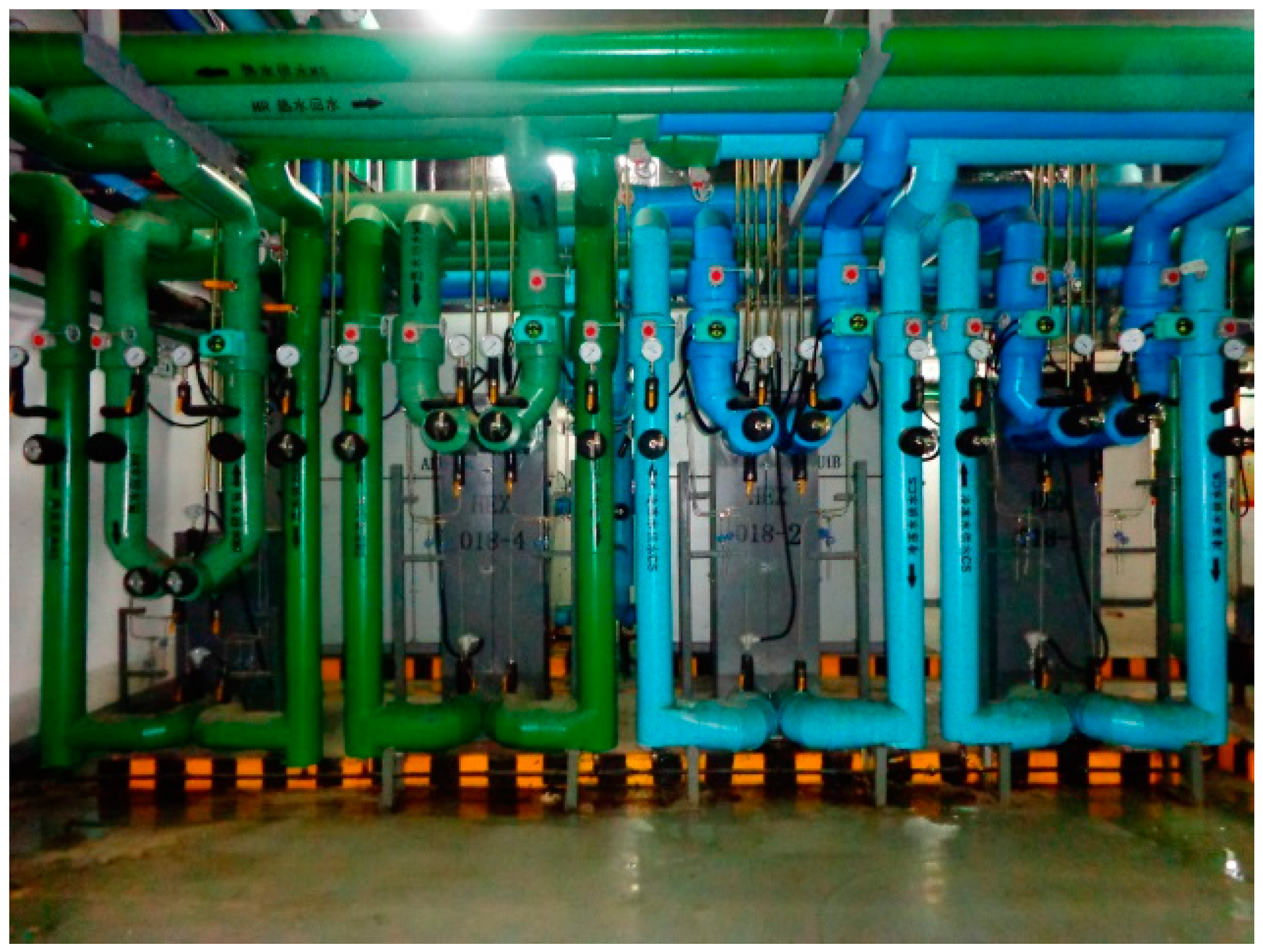
In order to validate the presented methods, a district heating system in Tianjin was tested. The system schematic is shown in Figure 2. The heat source and heating equipment in this district heating system are a ground-source heat pump (GSHP) and a fan coil (FC), respectively. In heating substations, the hot water from the heat source transfers heat to the cold water from the FC through the PHE (HISAKA PHE, RX-396B-TNUP-269, HISAKA Works (China) Co. Ltd., Shanghai, China). A picture of the PHE in the district heating system is shown in Figure 3.

For the inlet and outlet temperatures of PHE, the primary and secondary flow rates were measured every minute during the heating period of 2015–2016.

The inlet and outlet temperatures of PHE were measured by platinum resistance thermometers (PT100, ELECALL Electric Co. Ltd., Yueqing, China). The accuracy of the thermometers is ±(0.15 + 0.002 |t|) °C. The two flow rates were measured by means of Ultrasonic flow meters (Fluke Corporation, Washington, DC, USA). The accuracy of the flow meters is ±2%. The test data is recorded by a data logger.

According to [18], uncertainty analysis is conducted to validate the test results. The uncertainty of temperature is established to be ±2.06%. The uncertainty of the convective heat transfer coefficients is calculated to be ±3.12%. The overall heat transfer coefficient calculated by the temperature and flow rate is approximately ±4.57%, an acceptable uncertain value range in engineering applications [19].

The parameters of the PHE are presented in

Table 1. Parameter of the plate heat exchanger (PHE).

Description	Symbol	Value	Unit
Channel length	$l_p$	125.25	cm
Channel width	$b_p$	45	cm
Distance between the PHE’s plates	${\delta }_p$	2	mm
Plate thickness	$H_p$	0.7	mm
Number of plates	N	269
Correlation parameter	$c_{Nu}$	0.18
Correlation parameter	$c_{Re}$	0.72
Correlation parameter	$c_{Pr}$	0.3
Heat conductivity (plate)	${\lambda }_p$	17	W/m/K
Hot fluid fouling factor	$R_{f,h}$	0.000017	m2·K/W
Cold fluid fouling factor	$R_{f,c}$	0.000017	m2·K/W

. The constant empirical parameters $c_{Nu}$, $c_{Re}$ and $c_{Pr}$ are estimated by the manufacturer’s data.

5. Results and Discussion

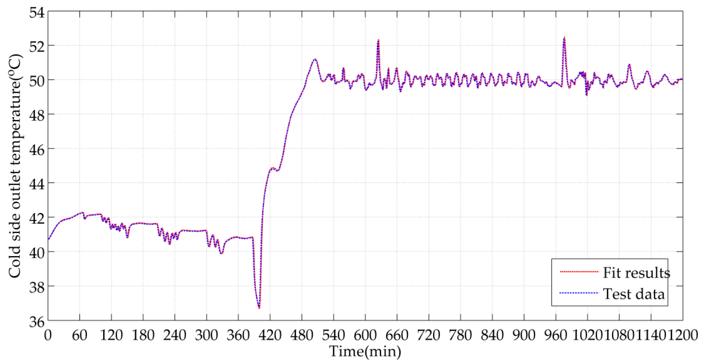
5.1. Parameter Matrix Identification

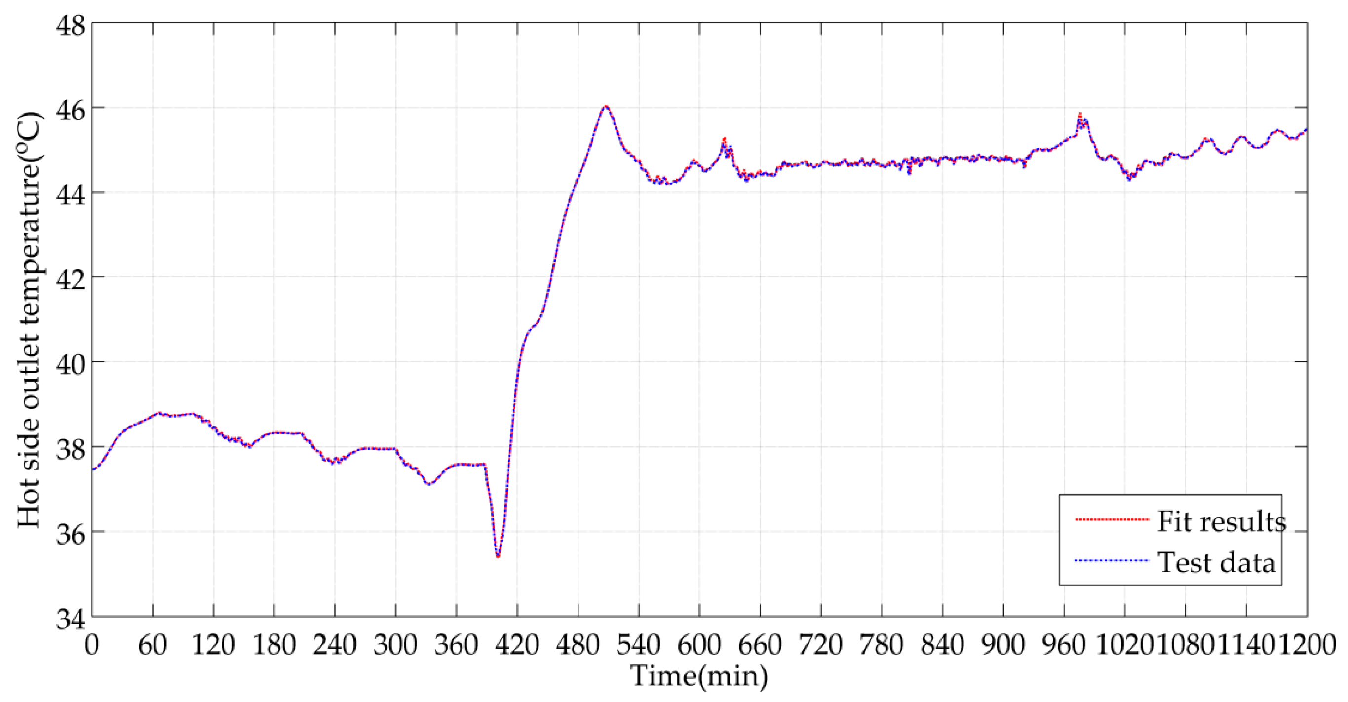
During the cold period, test data over 6 days (10–15 January 2016) were chosen to identify the parameter matrices. The data were rearranged as Equations (35)–(38), and parameter matrix identification was performed by applying Equations (42) and (43).

After obtaining the parameter matrices, the two outlet temperatures $T_{h,2}$ and $T_{c,2}$ were calculated from Equation (34), where the two inlet temperatures $T_{h,1}$ and $T_{c,1}$ and the two flow rates $u_h$ and $u_c$ were substituted with the test data as model inputs. The calculated two outlet temperatures $T_{h,2}$ and $T_{c,2}$ were compared with the test data. Figure 4 and Figure 5 show the comparison results in 20 h. The fit errors of outlet temperatures are calculated, and they are less than 0.2 °C.

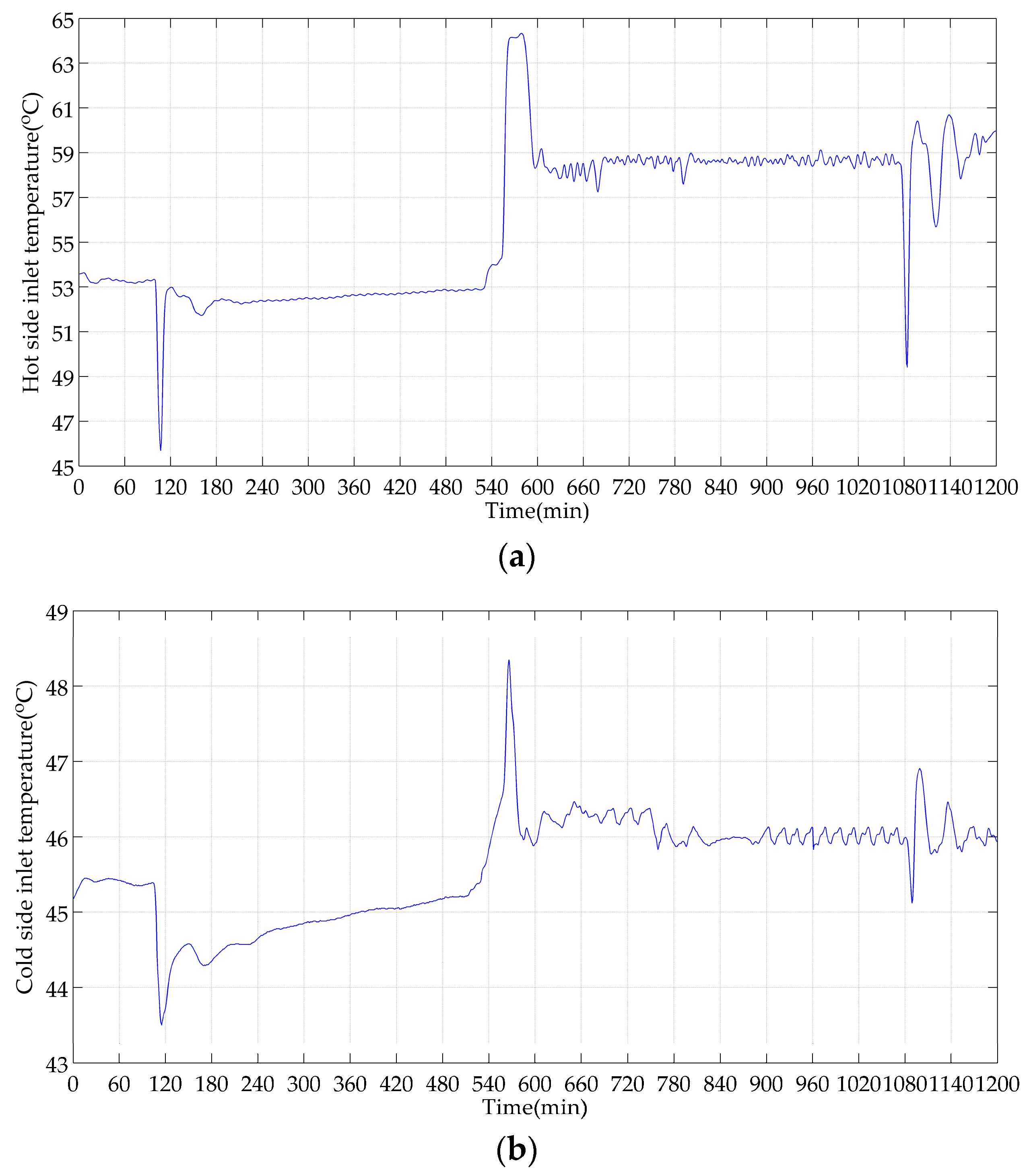
5.2. Validation of the Proposed Methods

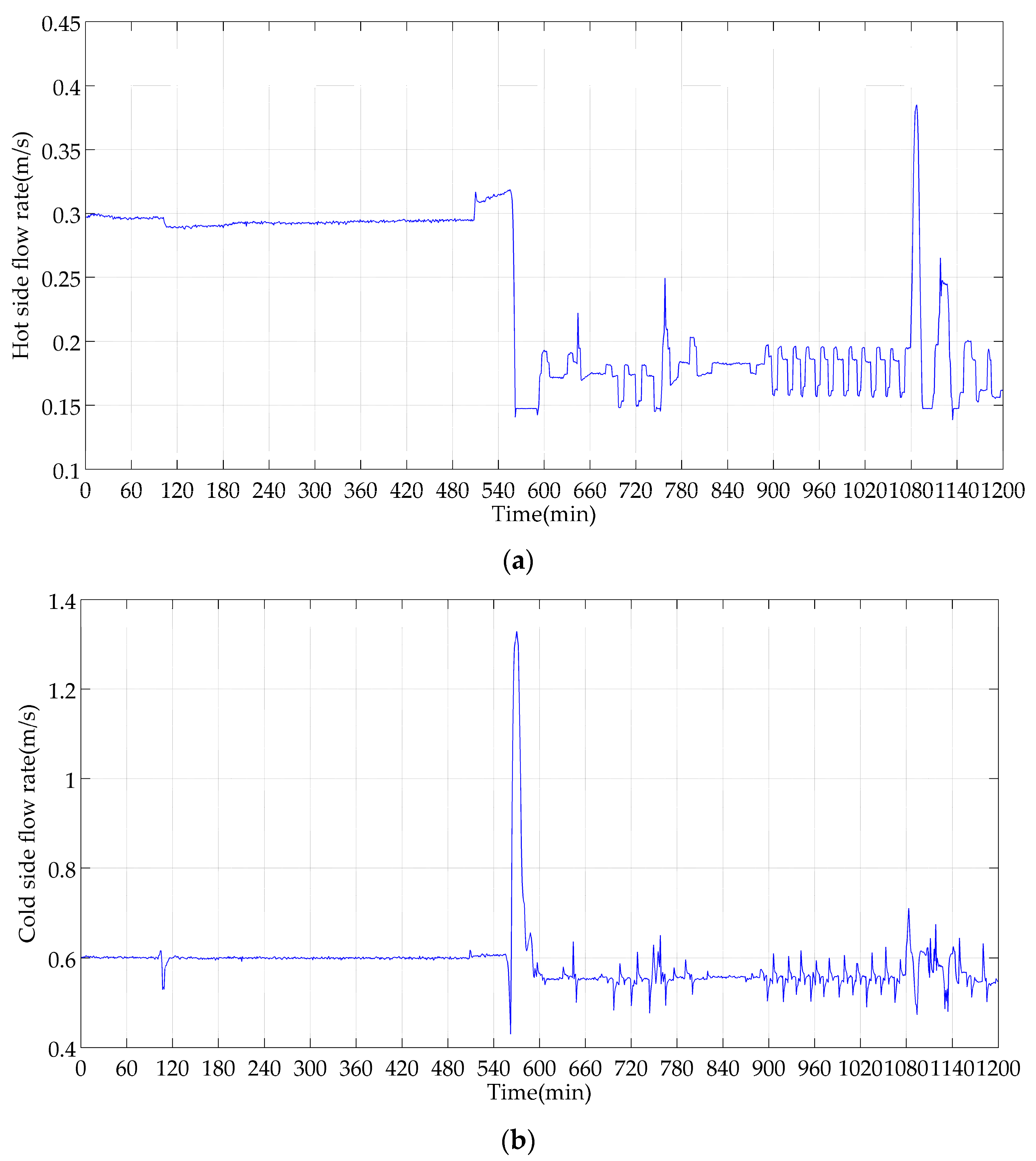
In order to validate the proposed methods, test data over 4 days (6–9 January 2016) were selected. The hot side flow rates ranged from about 0.15 to 0.4 m/s in this period.

For white-box method, the two outlet temperatures $T_{h,2}$ and $T_{c,2}$ were calculated based on Equation (23).

For grey-box method, according to Equation (34) the two outlet temperatures were calculated. The model inputs in 20 h, i.e., the two inlet temperatures $T_{h,1}$ and $T_{c,1}$ and the two flow rates $u_h$ and $u_c$, are depicted in Figure 6a,b and Figure 7a,b.

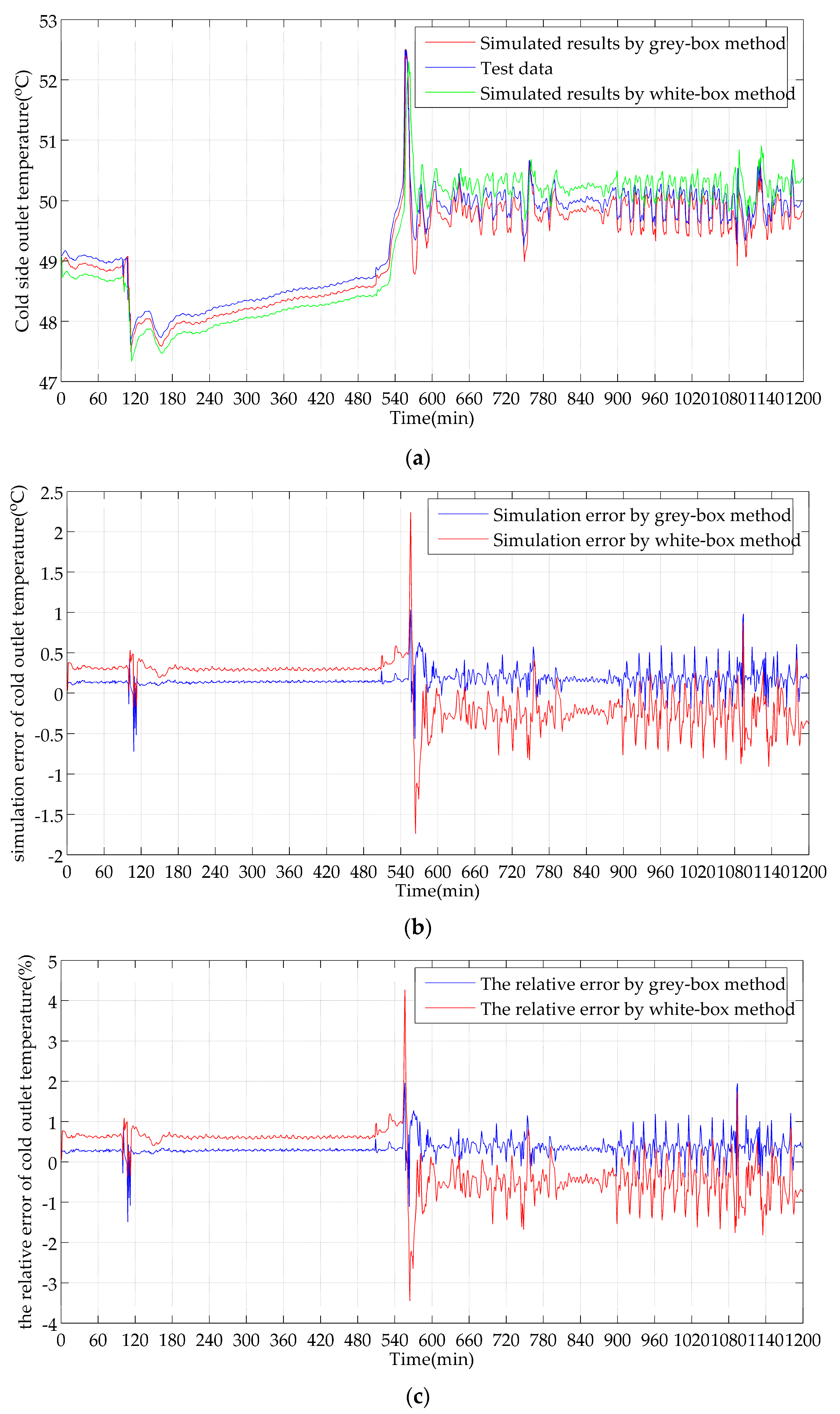
The plots of simulated vs. experimental outlet temperatures are presented in Figure 8a and Figure 9a. It can be seen that the simulated results by the grey-box method are closer to the test data than those obtained by the white-box method.

The simulation errors and of two outlet temperatures by the two methods are shown in Figure 8b and Figure 9b. It can be observed in the Figure 8b that the simulation error of hot outlet temperature $T_{h,2}$ by grey-box method is restricted within 0.5 °C, and the error by white-box method can be to a maximum of 2.6 °C. Figure 9b shows that the simulation error of cold outlet temperature $T_{c,2}$ by grey-box method is restricted within 1 °C, and the error by white-box method can be to a maximum of 2.2 °C.

The relative errors of the two methods with respect to the experimental data are shown in Figure 8c and Figure 9c. It can be seen that the relative errors of $T_{h,2}$ by grey-box method are less than 1%, and the error by white-box method is less than 5% in the majority from Figure 8c. Figure 9c shows that the relative error of $T_{c,2}$ by the grey-box method is also less than 2%, and the error by white-box method is less than 4% in the majority.

To acquire the quantificational validation of the method, a metric is put forward as follows [20]:

$$\mathrm{FIT}=1-\sqrt{{\displaystyle {\sum }_{i=1}^N}{\left({\widehat{y}}_i-y_i\right)}^2/{\displaystyle {\sum }_{i=1}^N}{\left(y_i-\frac{1}{N}{\displaystyle {\sum }_{i=1}^N{y}_i}\right)}^2}$$

(44)

where $y_i$ and ${\widehat{y}}_i$ denote the test data and the simulated results by model method, respectively. Equation (44) indicates that the value of FIT is smaller than 1.0. And the larger the value of FIT is, the more effective the method will be.

The FIT for outlet temperatures $T_{h,2}$ and $T_{c,2}$ by white-box method is 0.78 and 0.84, respectively. The obtained FIT by grey-box method is 0.96 and 0.94, respectively. Therefore, the simulated results by grey-box method are more accurate than the white-box method.

6. Conclusions

In this paper, a second-order state space model of PHEs was developed. Then the model was solved by the white-box method and grey-box method, respectively. In the white-box method, the linearization of the state space model was carried out by implicit difference scheme and the overall heat transfer coefficient was calculated with empirical correlation of Nusselt number. In the grey-box method, one-order Taylor series were used to make the linearization of the nonlinear state space model and a newly developed parameter matrix identification method was established.

The simulation results of outlet temperatures by the grey-box and white-box method respectively were compared with the test data. The plots of predicted outlet temperatures by the grey-box method were closer to the test data than those obtained by the white-box method. The comparison of the FIT by the two methods indicates that the grey-box method performs better than the white-box method.

When the PHE is in operation for a period in actual project, fouling resistance also impacts the overall heat transfer coefficient of PHEs. The grey-box method does not introduce any approximation on the heat transfer model, thus it can refrain from errors caused by differences of parameters in the Nusselt correlation. In addition, Equation (7) consists of a steady-state correlation, but the white-box method uses the Nusselt in a dynamic simulation of the operative variables of the PHE. Therefore the grey-box model can be used in transient simulation in a more appropriate way and it is more suitable and accurate for the predication of outlet temperatures than the white-box method for that. The presented results can produce useful guidelines for optimal control of heating system.

In our future works, based on the proposed grey-box method, the controller design and its application for the regulation of the flow rates of district heating systems will be investigated.