A Pontryagin Minimum Principle-Based Adaptive Equivalent Consumption Minimum Strategy for a Plug-in Hybrid Electric Bus on a Fixed Route

Abstract
:1. Introduction
1.1. Ground and Literature Review
1.2. Motivation
1.3. Contribution
1.4. Outline
2. Model Description
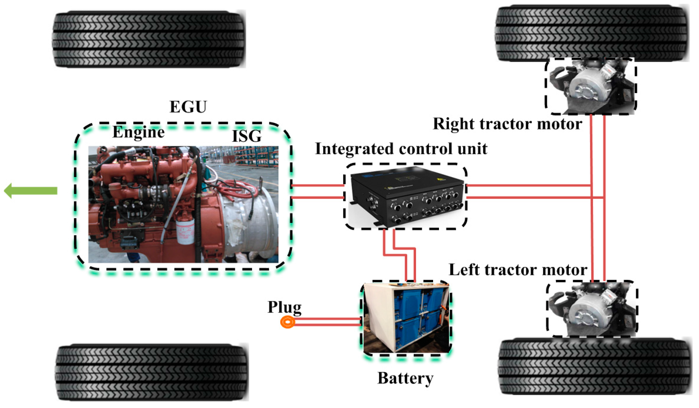
2.1. Powertrain Architecture and Model
2.1.1. Powertrain Architecture
2.1.2. Powertrain Model
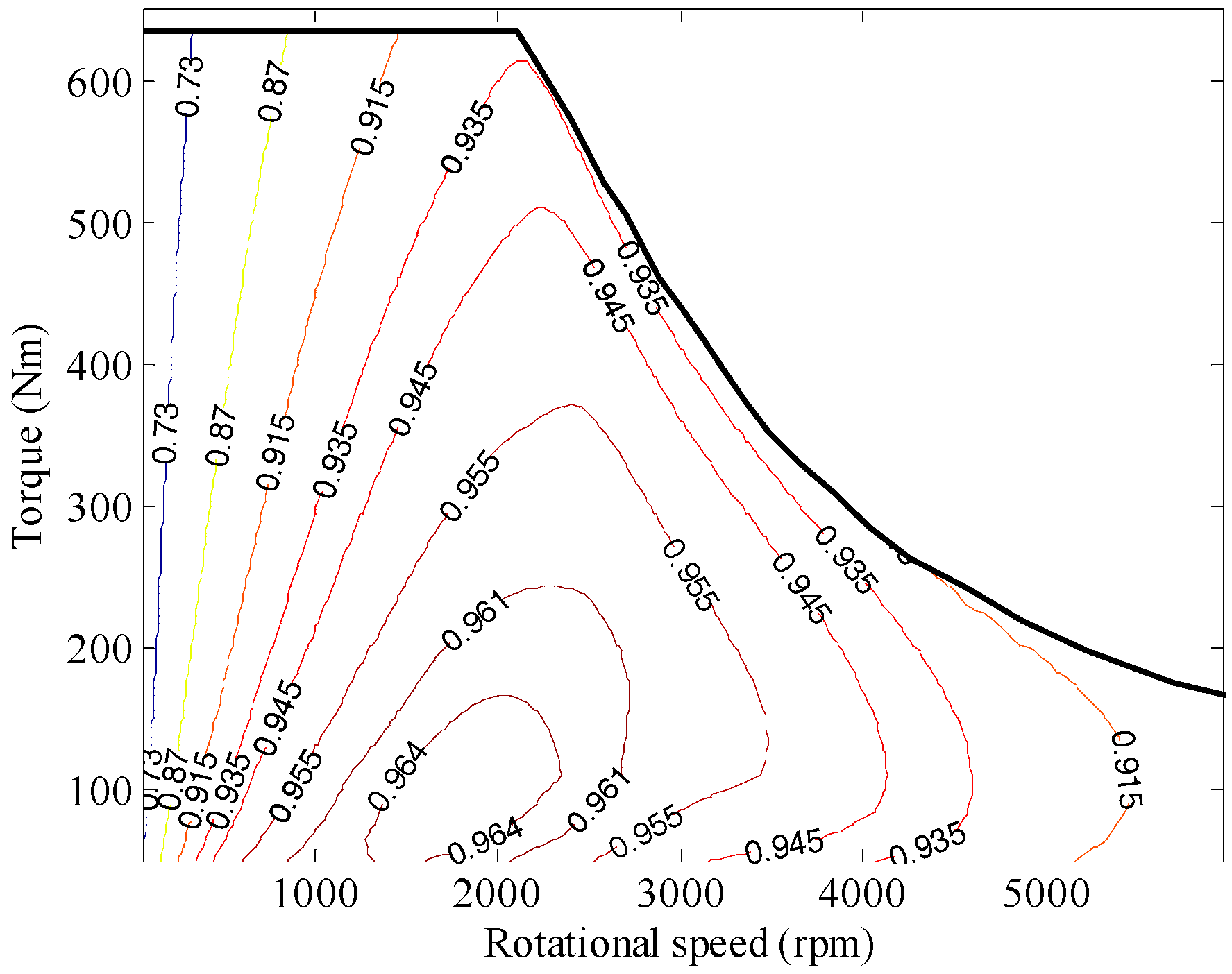
Motor Model
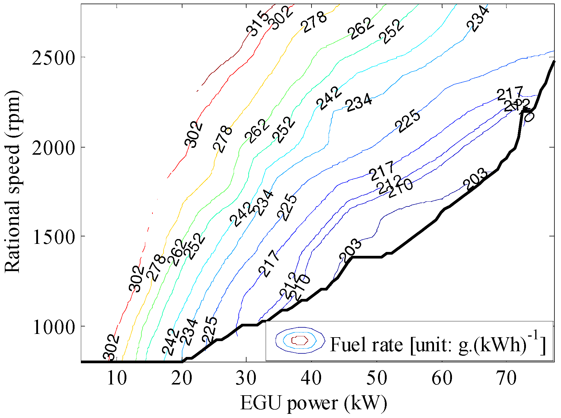
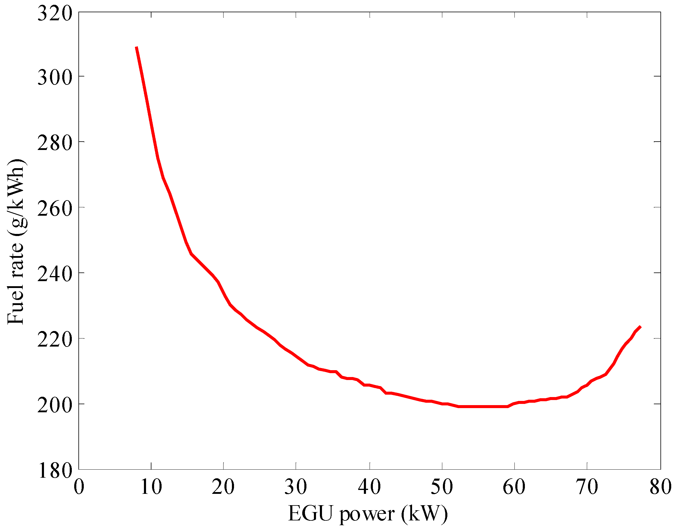
EGU Model
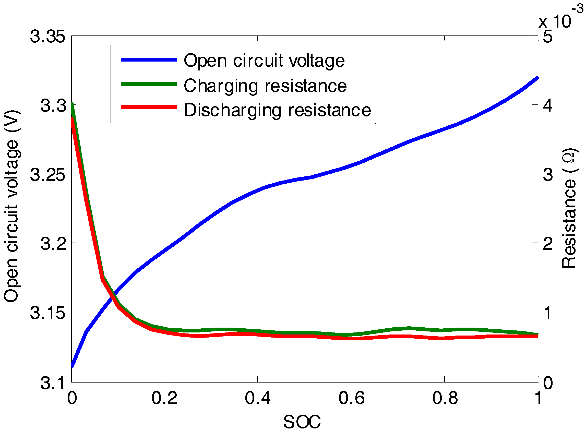
2.1.3. Battery Model
2.2. Longitudinal Dynamics
3. Pontryagin’s Minimum Principle
3.1. PMP
3.2. Numerical Solution
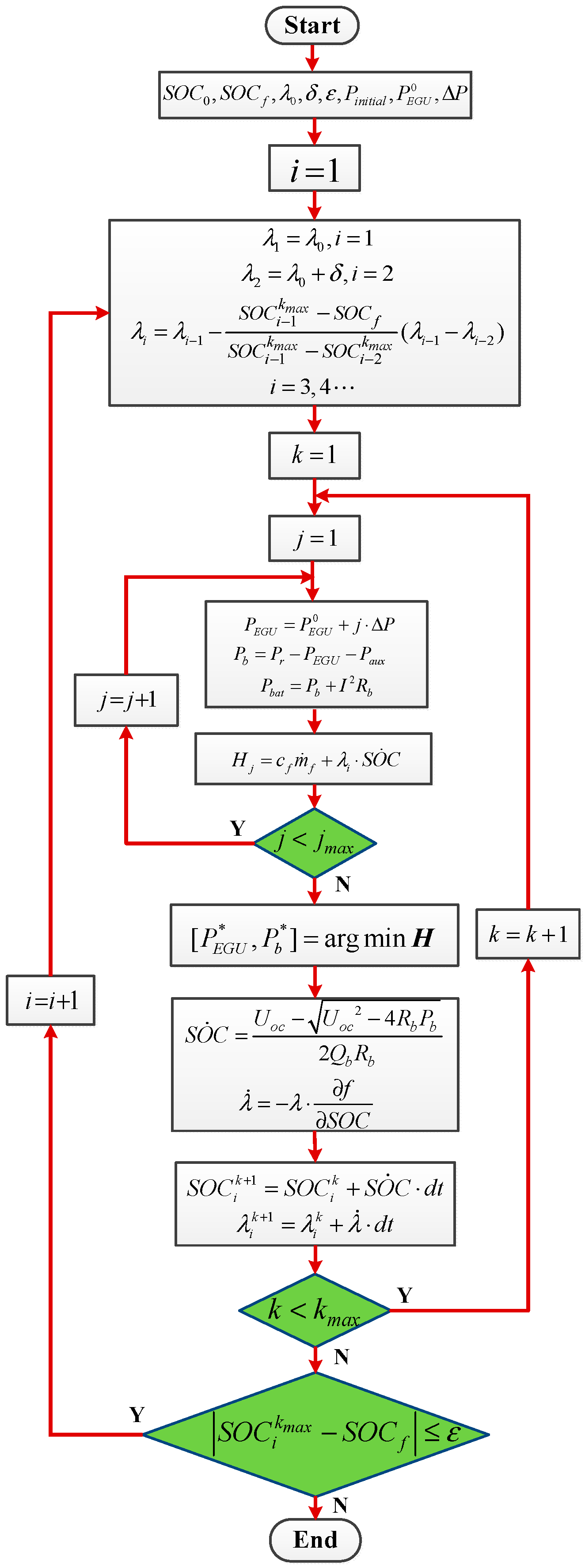
3.2.1. Shooting Method
3.2.2. Algorithm Flowchart
4. Adaptive ECMS
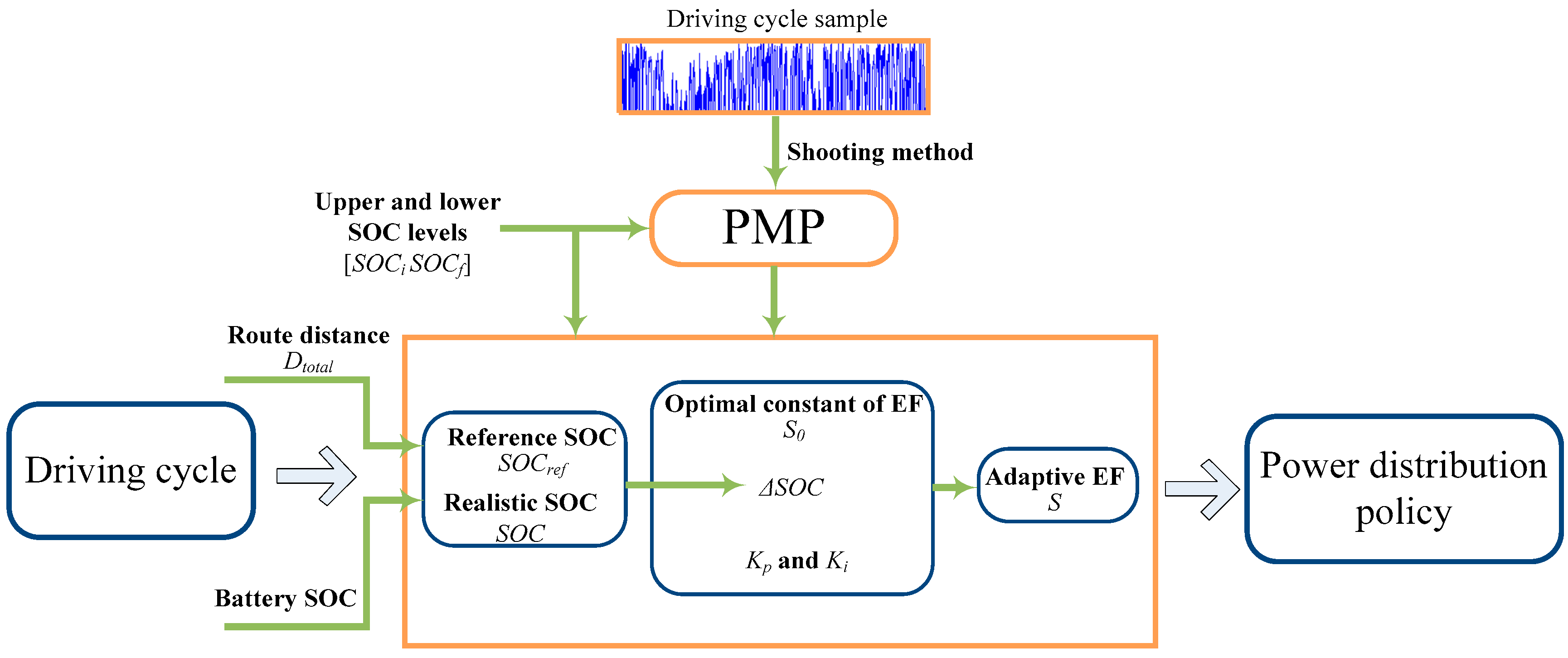
4.1. A-ECMS
4.2. Reference SOC
4.3. Adaptive Equivalence Factor
4.4. Optimal Stable Constant of EF
4.5. Scheme of A-ECMS
5. Validation and Discussion
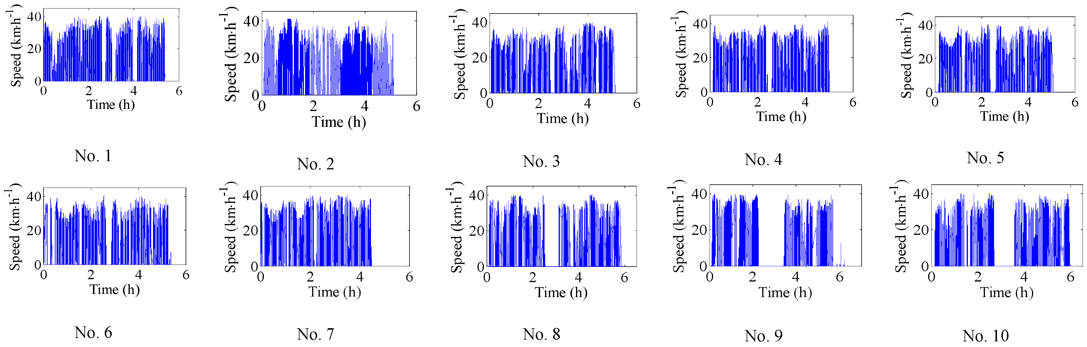
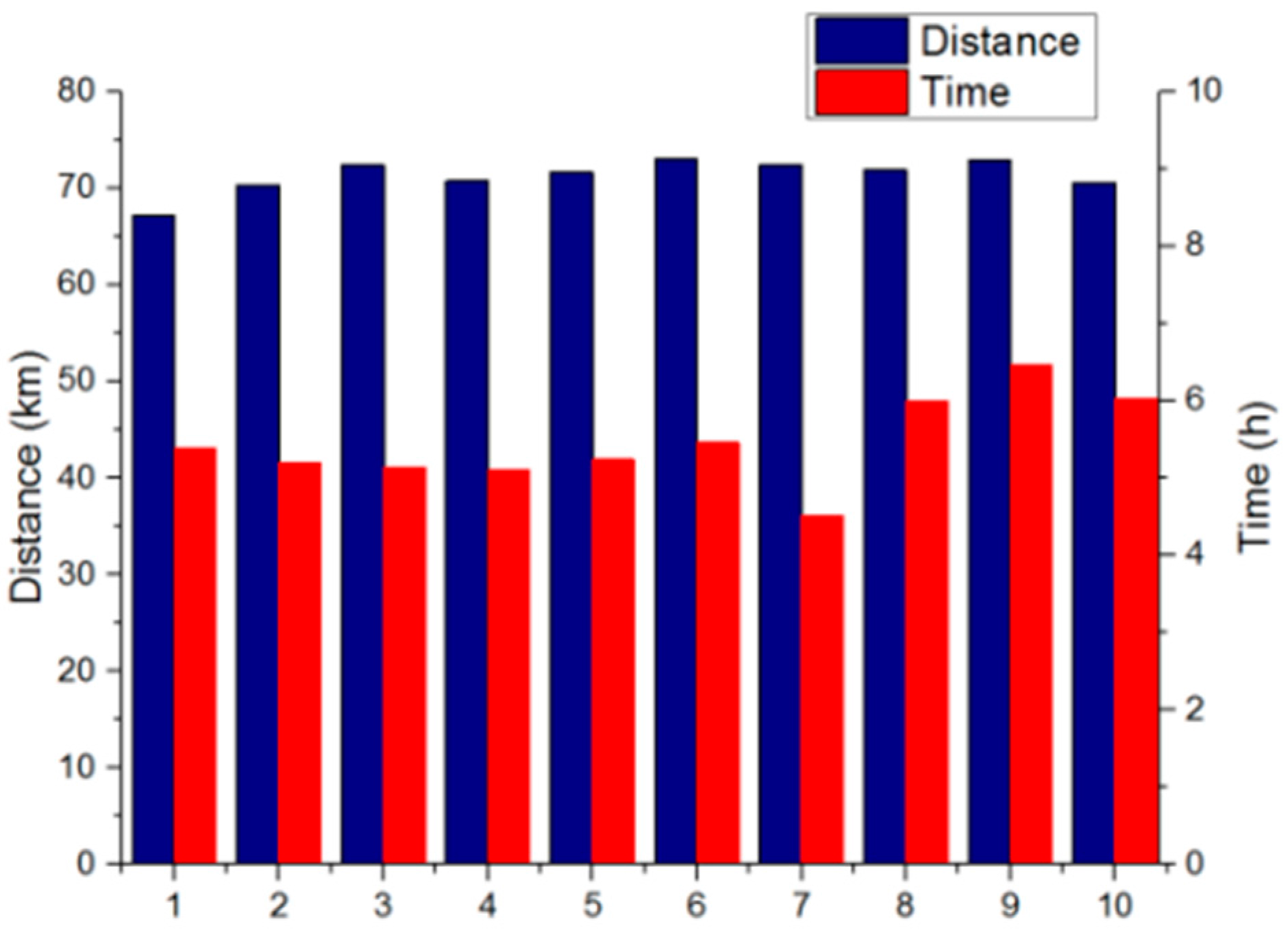
5.1. Route Discription
5.2. Calculation of Optimal Constant of EF
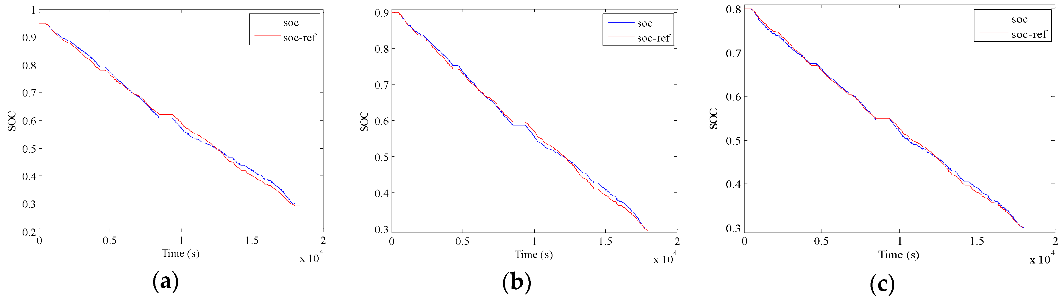
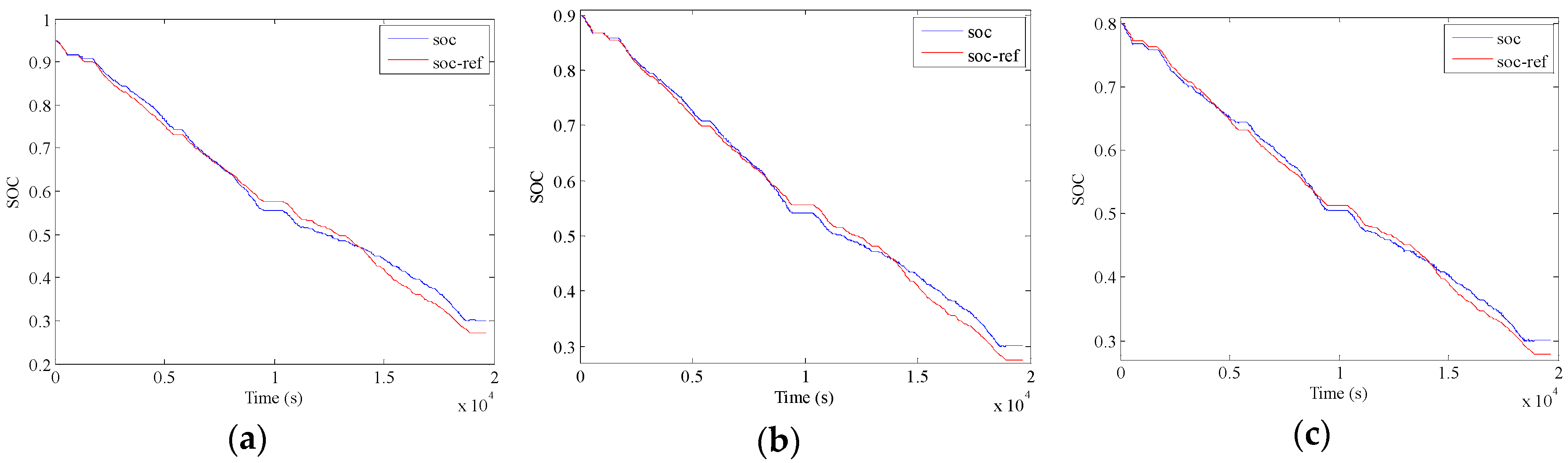
5.3. Validation of A-ECMS
6. Conclusions
- (1)
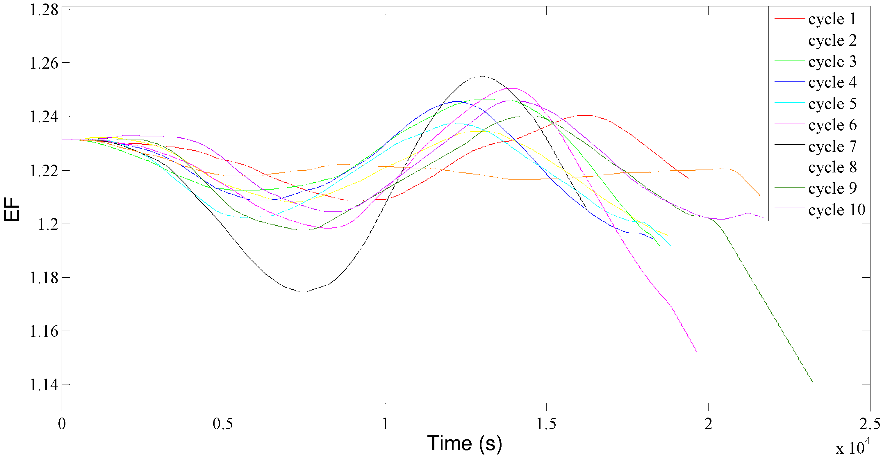
- The adaptive EF is considered as a combination of two parts including the major component and calibrating component, in which the major component defined as a constant has a dominate role in determining the EF while the latter denoted as a proportional and integral terms is designed to apply to the disparity of regular speeding profiles.
- (2)
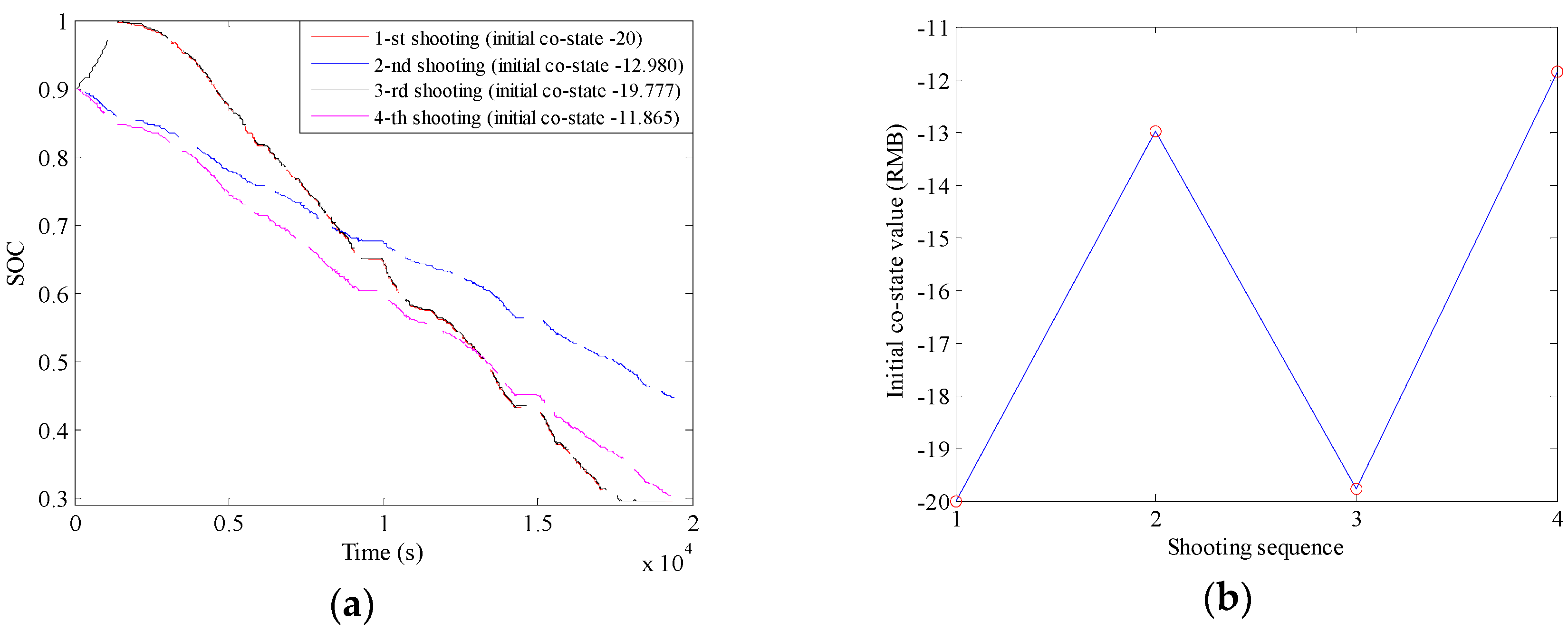
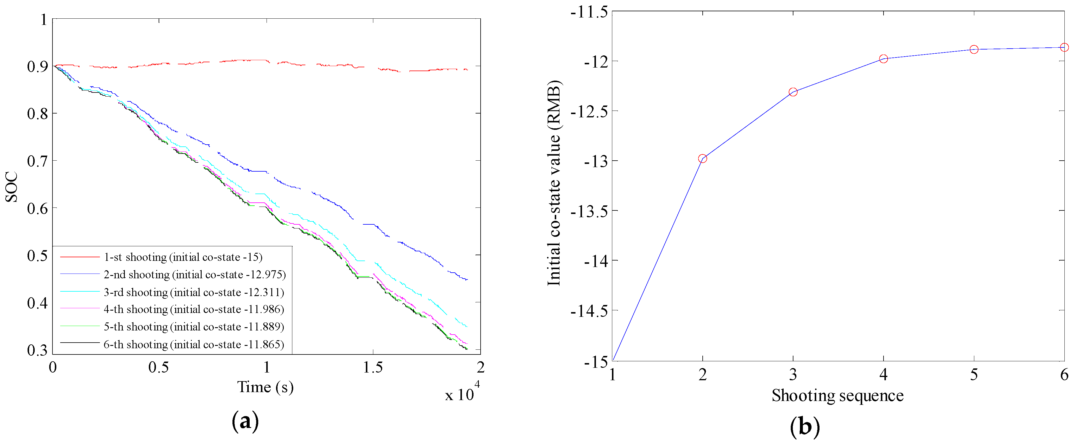
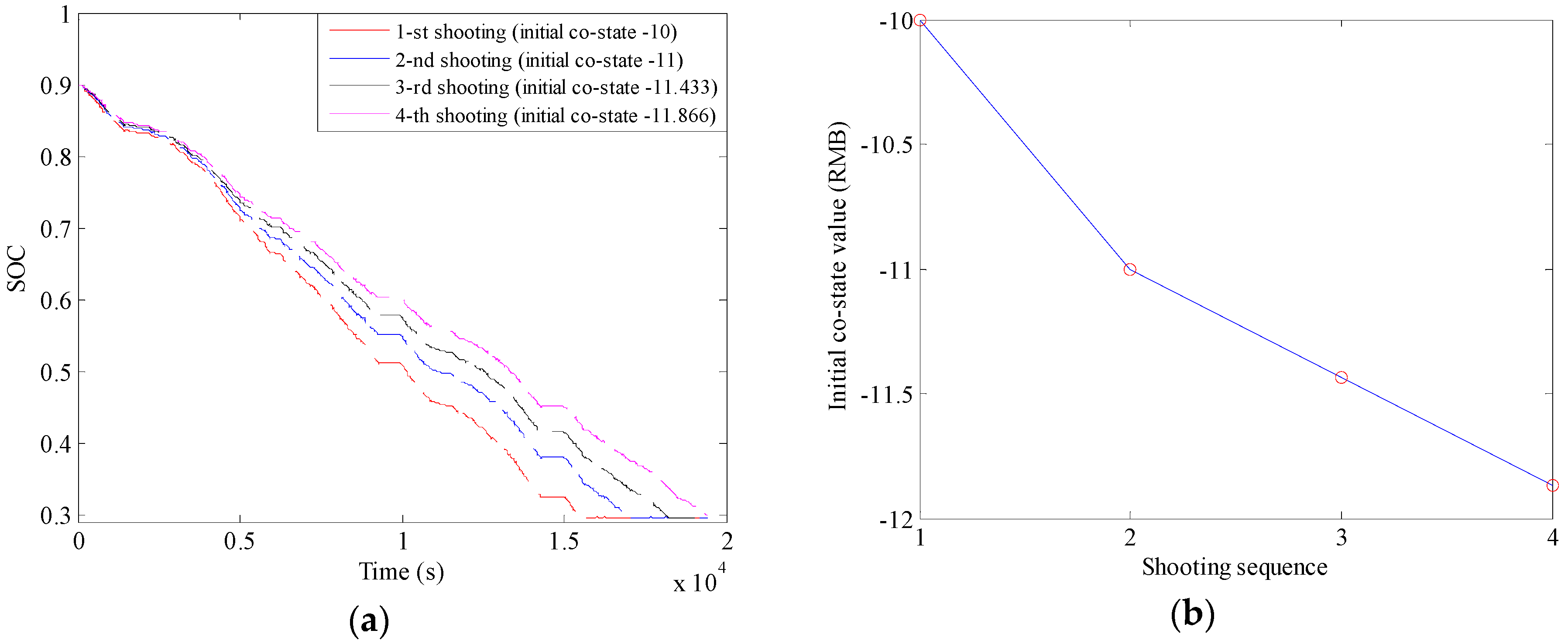
- The numerical solution of PMP strategy is acquired by using the shooting method, and the optimal initial co-state value captured in the last shooting operation is taken as the optimal stable constant, with which it is quite easy to tune the two PI coefficients. Meanwhile, to avoid repeatedly selecting of the initial co-state value in the beginning and obtain the optimal solution as soon as possible, the Secant method is employed to tune the initial co-state variable, which greatly reduces the shooting times and also exhibits a flexibility of adapting any appropriate initial co-state value.
- (3)
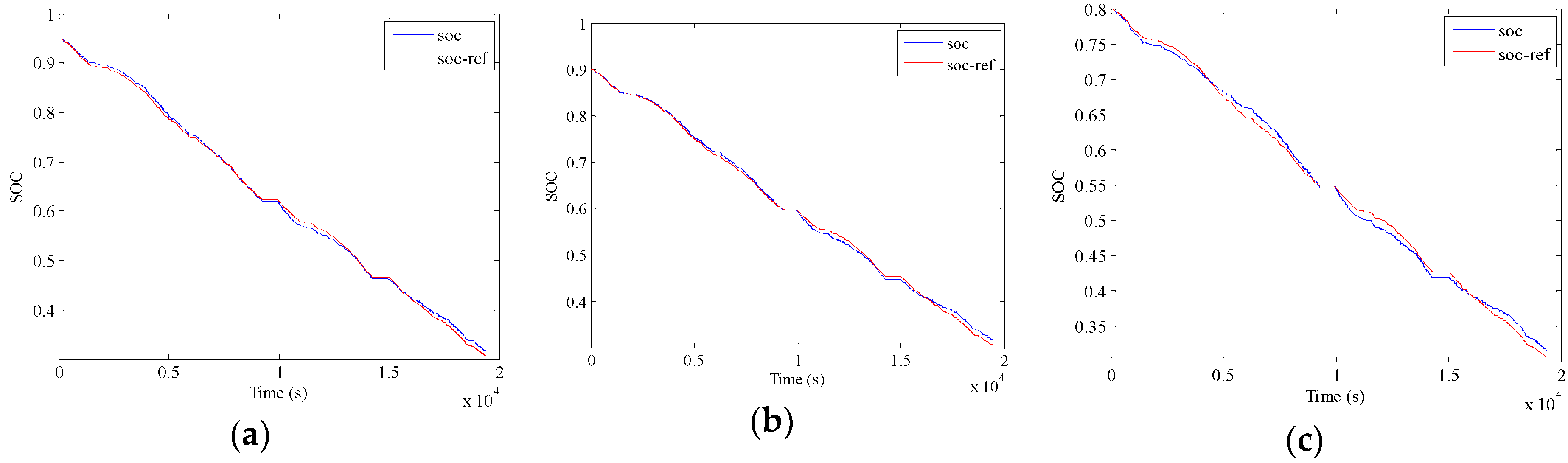
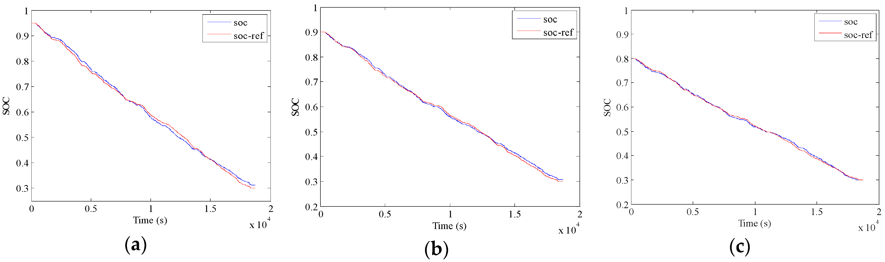
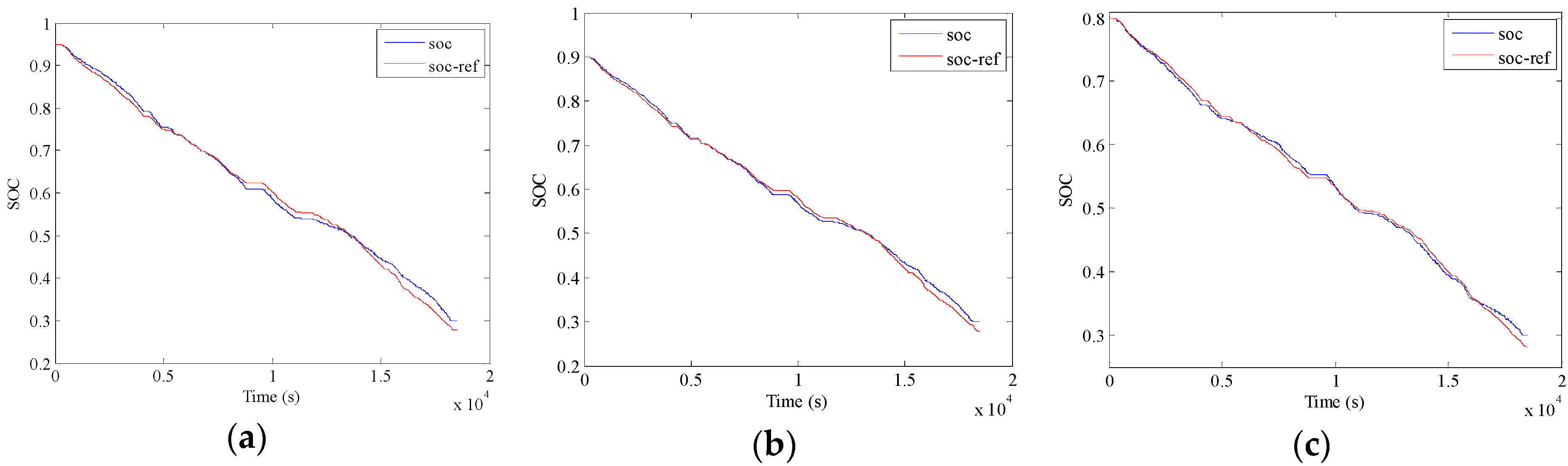
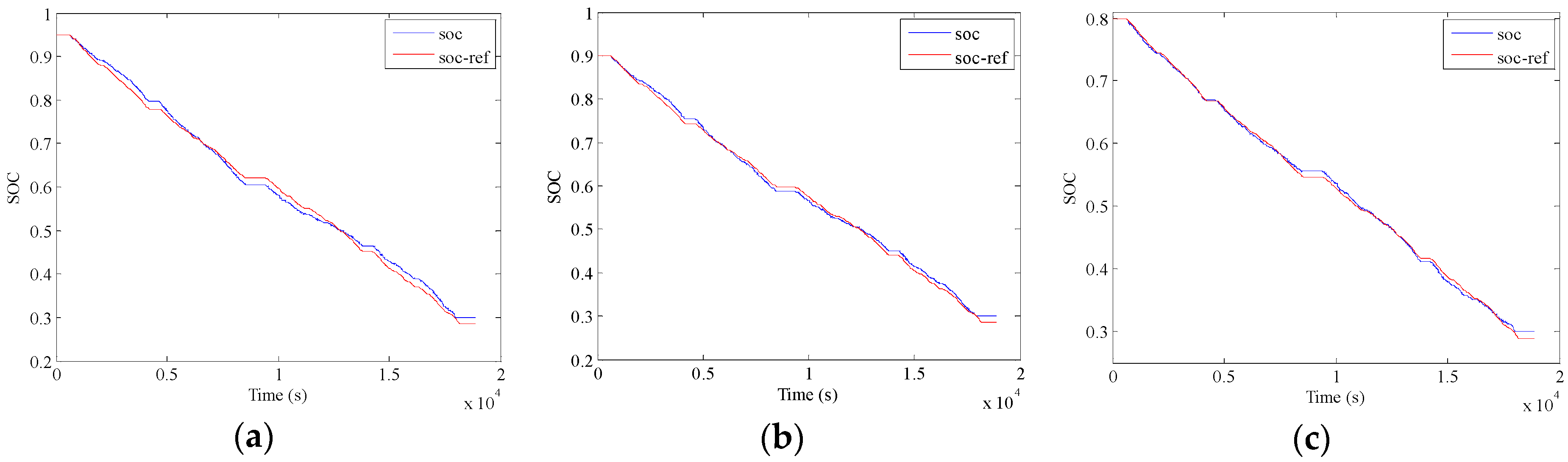
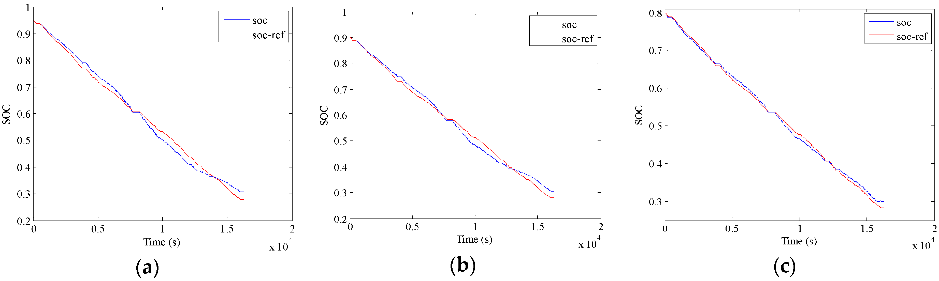
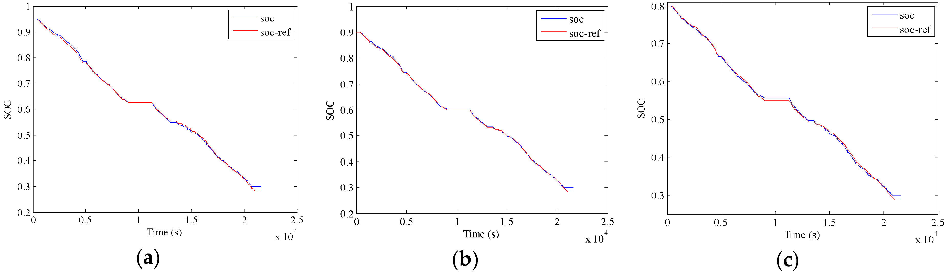
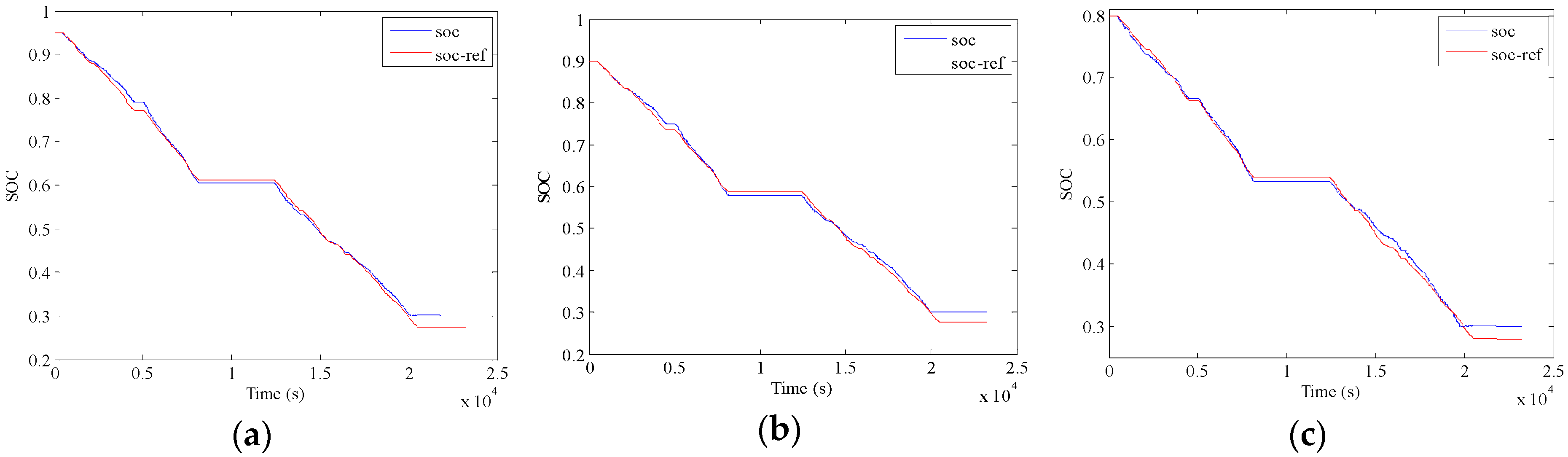
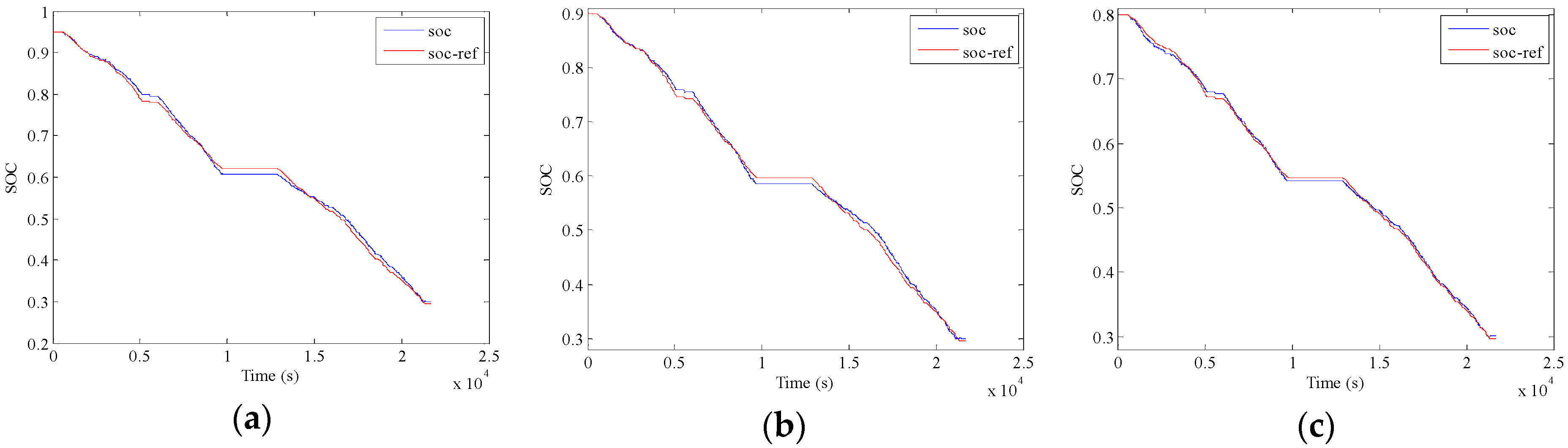
- The presented A-ECMS method is examined by ten successive speeding profiles, as well as with three initial SOC levels to simulate different charge levels. The results indicate almost the identical energy consumption cost compared to the DP and PMP algorithms, and the examination with different initial SOCs further demonstrates the robustness of the proposed method. Therefore, the proposed method offers an efficient approach of developing the A-ECMS strategy for the PHEBs with fixed routes.
Acknowledgments
Author Contributions
Conflicts of Interest
References
- Hu, X.; Martinez, C.M.; Yang, Y. Charging, power management, and battery degradation mitigation in plug-in hybrid electric vehicles: A unified cost-optimal approach. Mech. Syst. Signal Process. 2017, 87, 4–16. [Google Scholar] [CrossRef]
- Liu, Y.; Li, J.; Ye, M.; Qin, D.; Zhang, Y.; Lei, Z. Optimal Energy Management Strategy for a Plug-in Hybrid Electric Vehicle Based on Road Grade Information. Energies 2017, 10, 412. [Google Scholar] [CrossRef]
- Gonder, J.; Markel, T. Energy Management Strategies for Plug-In Hybrid Electric Vehicles; SAE Permissions: Warrendale, PA, USA, 2007. [Google Scholar]
- Hu, X.; Jiang, J.; Egardt, B.; Cao, D. Advanced power-source integration in hybrid electric vehicles: Multicriteria optimization approach. IEEE Trans. Ind. Electron. 2015, 62, 7847–7858. [Google Scholar] [CrossRef]
- Serrao, L.; Onori, S.; Rizzoni, G. ECMS as a realization of Pontryagin’s minimum principle for HEV control. In Proceedings of the American Control Conference, St. Louis, MO, USA, 10–12 June 2009; pp. 3964–3969. [Google Scholar]
- Khayyam, H.; Bab-Hadiashar, A. Adaptive intelligent energy management system of plug-in hybrid electric vehicle. Energy 2014, 69, 319–335. [Google Scholar] [CrossRef]
- Schouten, N.J.; Salman, M.A.; Kheir, N.A. Fuzzy logic control for parallel hybrid vehicles. IEEE Trans. Control Syst. Technol. 2002, 10, 460–468. [Google Scholar] [CrossRef]
- Lin, C.C.; Peng, H.; Grizzle, J.W.; Kong, J.-M. Power management strategy for a parallel hybrid electric truck. IEEE Trans. Control Syst. Technol. 2003, 11, 839–849. [Google Scholar]
- Pisu, P.; Rizzoni, G. A comparative study of supervisory control strategies for hybrid electric vehicles. IEEE Trans. Control Syst. Technol. 2007, 15, 506–518. [Google Scholar] [CrossRef]
- Kim, N.; Cha, S.; Peng, H. Optimal control of hybrid electric vehicles based on Pontryagin’s minimum principle. IEEE Trans. Control Syst. Technol. 2011, 19, 1279–1287. [Google Scholar]
- Xu, L.; Yang, F.; Li, J.; Ouyang, M.; Hua, J. Real time optimal energy management strategy targeting at minimizing daily operation cost for a plug-in fuel cell city bus. Int. J. Hydrogen Energy 2012, 37, 15380–15392. [Google Scholar] [CrossRef]
- Hou, C.; Ouyang, M.; Xu, L.; Wang, H. Approximate Pontryagin’s minimum principle applied to the energy management of plug-in hybrid electric vehicles. Appl. Energy 2014, 115, 174–189. [Google Scholar] [CrossRef]
- Lacandia, F.; Tribioli, L.; Onori, S.; Rizzoni, G. Adaptive energy management strategy calibration in PHEVs based on a sensitivity study. SAE Int. J. Alt. Power 2013, 2, 443–455. [Google Scholar] [CrossRef]
- Zhang, F.; Liu, H.; Hu, Y.; Xi, J. A supervisory control algorithm of hybrid electric vehicle based on adaptive equivalent consumption minimization strategy with fuzzy PI. Energies 2016, 9, 919. [Google Scholar] [CrossRef]
- Xu, L.; Li, J.; Ouyang, M.; Hua, J.; Yang, G. Multi-mode control strategy for fuel cell electric vehicles regarding fuel economy and durability. Int. J. Hydrogen Energy 2014, 39, 2374–2389. [Google Scholar] [CrossRef]
- Tang, L.; Rizzoni, G.; Onori, S. Energy management strategy for HEVs including battery life optimization. IEEE Trans. Transp. Electrification 2015, 1, 211–222. [Google Scholar] [CrossRef]
- Tulpule, P.; Marano, V.; Rizzoni, G. Energy management for plug-in hybrid electric vehicles using equivalent consumption minimization strategy. Int. J. Electric Hybrid Veh. 2010, 2, 329–350. [Google Scholar] [CrossRef]
- Zhang, F.; Xi, J.; Langari, R. Real-Time energy management strategy based on velocity forecasts using V2V and V2I communications. IEEE Trans. Intell. Transp. Syst. 2017, 18, 416–430. [Google Scholar] [CrossRef]
- Sciarretta, A.; Back, M.; Guzzella, L. Optimal control of parallel hybrid electric vehicles. IEEE Trans. Control Syst. Technol. 2004, 12, 352–363. [Google Scholar] [CrossRef]
- Onori, S.; Serrao, L. On Adaptive-ECMS strategies for hybrid electric vehicles. In Proceedings of the International Scientific Conference on Hybrid and Electric Vehicles, Malmaison, France, 6–7 December 2011. [Google Scholar]
- Gu, B.; Rizzoni, G. An adaptive algorithm for hybrid electric vehicle energy management based on driving pattern recognition. In Proceedings of the International Mechanical Engineering Congress and Exposition, Chicago, IL, USA, 5–10 November 2006; pp. 249–258. [Google Scholar]
- Yokoi, Y.; Ichikawa, S.; Doki, S.; Okuma, S.; Naitou, T.; Miki, N. Driving pattern prediction for an energy management system of hybrid electric vehicles in a specific driving course. In Proceedings of the 30th Annual Conference of IEEE Industrial Electronics Society, Busan, Korea, 2–6 November 2004; pp. 1727–1732. [Google Scholar]
- Onori, S.; Tribioli, L. Adaptive Pontryagin’s Minimum Principle supervisory controller design for the plug-in hybrid GM Chevrolet Volt. Appl. Energy 2015, 147, 224–234. [Google Scholar] [CrossRef]
- Sivertsson, M.; Eriksson, L. Design and evaluation of energy management using map-based ECMS for the PHEV benchmark. Oil Gas Sci. Technol. 2015, 70, 195–211. [Google Scholar] [CrossRef]
- Larsson, V.; Johannesson, L.; Egardt, B.; Lasson, A. Benefit of route recognition in energy management of plug-in hybrid electric vehicles. In Proceedings of the American Control Conference, Montreal, QC, Canada, 27–29 June 2012; pp. 1314–1320. [Google Scholar]
- Li, L.; Yang, C.; Zhang, Y.; Zhang, L.; Song, J. Correctional DP-based energy management strategy of plug-in hybrid electric bus for city-bus route. IEEE Trans. Veh. Technol. 2015, 64, 2792–2803. [Google Scholar] [CrossRef]
- Han, J.; Park, Y.; Kum, D. Optimal adaptation of equivalent factor of equivalent consumption minimization strategy for fuel cell hybrid electric vehicles under active state inequality constraints. J. Power Sources 2014, 267, 491–502. [Google Scholar] [CrossRef]
- Borhan, H.; Vahidi, A.; Phillips, A.M. MPC-based energy management of a power-split hybrid electric vehicle. IEEE Trans. Control Syst. Technol. 2012, 20, 593–603. [Google Scholar] [CrossRef]
- Hemi, H.; Ghouili, J.; Cheriti, A. Combination of Markov chain and optimal control solved by Pontryagin’s Minimum Principle for a fuel cell/supercapacitor vehicle. Energy Convers. Manag. 2015, 91, 387–393. [Google Scholar] [CrossRef]
- Xie, S.; He, H.; Peng, J. An energy management strategy based on stochastic model predictive control for plug-in hybrid electric buses. Appl. Energy 2017, 196, 279–288. [Google Scholar] [CrossRef]
- Li, G.; Zhang, J.; He, H. Battery SOC constraint comparison for predictive energy management of plug-in hybrid electric bus. Appl. Energy 2017, 194, 578–587. [Google Scholar] [CrossRef]
- Li, L.; You, S.; Yang, C.; Yan, B.; Song, J.; Chen, Z. Driving-behavior-aware stochastic model predictive control for plug-in hybrid electric buses. Appl. Energy 2016, 162, 868–879. [Google Scholar] [CrossRef]
- Sun, C.; Hu, X.; Moura, S.J.; Sun, F. Comparison of velocity forecasting strategies for predictive control in HEVs. In Proceedings of the ASME 2014 Dynamic Systems and Control Conference, San Antonio, TX, USA, 22–24 October 2014. [Google Scholar]
- Sun, C.; Moura, S.J.; Hu, X.; Hedrick, J.K.; Sun, F. Dynamic traffic feedback data enabled energy management in plug-in hybrid electric vehicles. IEEE Trans. Control Syst. Technol. 2015, 23, 1075–1086. [Google Scholar]
- Johnson, V.H. Battery performance models in ADVISOR. J. Power Sources 2002, 110, 321–329. [Google Scholar] [CrossRef]


| Item | Parameter | Value |
|---|---|---|
| Vehicle | Curb weight (kg) | 13,500 |
| Reducer ratio | 13.9 | |
| Engine | Displacement (L) | 4.2 |
| Rated power (kW) | 88 | |
| Max speed (rpm) | 2800 | |
| ISG | Max power (kW) | 130 |
| Max torque (Nm) | 500 | |
| Max speed (rpm) | 6000 | |
| Driving motor | Max power (kW) | 150 |
| Max torque (Nm) | 650 | |
| Max speed (rpm) | 6000 | |
| Battery | Capacity (Ah) | 120 |
| Battery total voltage (V) | 537.6 |
| Parameter | Value | Parameter | Value | Parameter | Value |
|---|---|---|---|---|---|
| (Yuan·m−3) | 3.7 | SOC upper level | 0.9 | −20/−15/−10 | |
| (Yuan·kWh−1) | 0.8 | SOC lower level | 0.3 | −1.0 | |
| (kW) | 0.5 | 1 | 0.001 |
| Cycle Number | |||||
|---|---|---|---|---|---|
| = −20 | = −15 | = −10 | |||
| 1 | −11.865 | −11.866 | −11.865 | −11.865 | 1.2299 |
| 2 | −11.909 | −11.909 | −11.909 | −11.909 | 1.2308 |
| 3 | −12.218 | −12.217 | −12.218 | −12.218 | 1.2367 |
| 4 | −12.049 | −12.045 | −12.047 | −12.047 | 1.2334 |
| 5 | −11.941 | −11.940 | −11.940 | −11.940 | 1.2314 |
| 6 | −12.001 | −11.996 | −12.000 | −11.999 | 1.2325 |
| 7 | −11.846 | −11.847 | −11.846 | −11.846 | 1.2295 |
| 8 | −11.979 | −11.975 | −11.975 | −11.976 | 1.2321 |
| 9 | −12.101 | −12.101 | −12.102 | −12.101 | 1.2345 |
| 10 | −11.953 | −11.953 | −11.956 | −11.954 | 1.2316 |
| Cycle Number | Gas Consumption (m3) | Electricity Consumption (kWh) | Final SOC | Total Energy Consumption Cost (Yuan) | ||
|---|---|---|---|---|---|---|
| A-ECMS | PMP | DP | ||||
| 1 | 3.79 | 41.96 | 0.317 | 47.60 | 47.40 | 47.87 |
| 2 | 3.35 | 42.19 | 0.313 | 46.14 | 45.97 | 46.59 |
| 3 | 3.71 | 43.51 | 0.300 | 48.54 | 48.57 | 49.26 |
| 4 | 3.90 | 43.42 | 0.301 | 49.16 | 49.17 | 49.55 |
| 5 | 3.50 | 44.02 | 0.300 | 48.16 | 48.28 | 48.83 |
| 6 | 3.58 | 43.77 | 0.301 | 48.28 | 48.29 | 48.71 |
| 7 | 4.03 | 42.57 | 0.308 | 48.99 | 48.76 | 49.18 |
| 8 | 3.39 | 43.88 | 0.300 | 47.66 | 47.79 | 48.42 |
| 9 | 3.84 | 44.45 | 0.301 | 49.78 | 49.99 | 50.34 |
| 10 | 3.57 | 43.55 | 0.300 | 48.04 | 48.08 | 48.47 |
| Cycle Number | Gas Consumption (m3) | Electricity Consumption (kWh) | Final SOC | Total Energy Consumption Cost (Yuan) | ||
|---|---|---|---|---|---|---|
| A-ECMS | PMP | DP | ||||
| 1 | 4.69 | 38.57 | 0.318 | 48.21 | 47.99 | 48.42 |
| 2 | 4.11 | 39.31 | 0.306 | 46.64 | 46.56 | 47.11 |
| 3 | 4.47 | 40.62 | 0.300 | 49.04 | 49.18 | 49.83 |
| 4 | 4.68 | 40.43 | 0.301 | 49.68 | 49.78 | 50.12 |
| 5 | 4.27 | 41.05 | 0.300 | 48.66 | 48.87 | 49.41 |
| 6 | 4.38 | 40.69 | 0.301 | 48.77 | 48.89 | 49.27 |
| 7 | 4.88 | 39.32 | 0.306 | 49.51 | 49.35 | 49.74 |
| 8 | 4.22 | 40.73 | 0.300 | 48.22 | 48.39 | 48.97 |
| 9 | 4.62 | 41.51 | 0.301 | 50.30 | 50.59 | 50.92 |
| 10 | 4.37 | 40.50 | 0.300 | 48.57 | 48.68 | 49.04 |
| Cycle Number | Gas Consumpiton (m3) | Electricity Consumption (kWh) | Final SOC | Total Energy Consumption Cost (Yuan) | ||
|---|---|---|---|---|---|---|
| A-ECMS | PMP | DP | ||||
| 1 | 6.44 | 32.01 | 0.32 | 49.45 | 49.23 | 49.62 |
| 2 | 5.65 | 33.54 | 0.30 | 47.72 | 47.81 | 48.33 |
| 3 | 6.42 | 33.30 | 0.30 | 50.41 | 50.44 | 51.10 |
| 4 | 6.48 | 33.67 | 0.30 | 50.92 | 51.03 | 51.35 |
| 5 | 6.17 | 33.92 | 0.30 | 49.96 | 50.12 | 50.61 |
| 6 | 6.06 | 34.38 | 0.30 | 49.92 | 50.14 | 50.52 |
| 7 | 6.37 | 33.67 | 0.30 | 50.49 | 50.59 | 50.97 |
| 8 | 6.12 | 33.61 | 0.30 | 49.54 | 49.63 | 50.21 |
| 9 | 6.31 | 35.15 | 0.30 | 51.48 | 51.85 | 52.16 |
| 10 | 6.25 | 33.41 | 0.30 | 49.86 | 49.92 | 50.27 |
© 2017 by the authors. Licensee MDPI, Basel, Switzerland. This article is an open access article distributed under the terms and conditions of the Creative Commons Attribution (CC BY) license (http://creativecommons.org/licenses/by/4.0/).
Share and Cite
Xie, S.; Li, H.; Xin, Z.; Liu, T.; Wei, L. A Pontryagin Minimum Principle-Based Adaptive Equivalent Consumption Minimum Strategy for a Plug-in Hybrid Electric Bus on a Fixed Route. Energies 2017, 10, 1379. https://doi.org/10.3390/en10091379
Xie S, Li H, Xin Z, Liu T, Wei L. A Pontryagin Minimum Principle-Based Adaptive Equivalent Consumption Minimum Strategy for a Plug-in Hybrid Electric Bus on a Fixed Route. Energies. 2017; 10(9):1379. https://doi.org/10.3390/en10091379
Chicago/Turabian StyleXie, Shaobo, Huiling Li, Zongke Xin, Tong Liu, and Lang Wei. 2017. "A Pontryagin Minimum Principle-Based Adaptive Equivalent Consumption Minimum Strategy for a Plug-in Hybrid Electric Bus on a Fixed Route" Energies 10, no. 9: 1379. https://doi.org/10.3390/en10091379
APA StyleXie, S., Li, H., Xin, Z., Liu, T., & Wei, L. (2017). A Pontryagin Minimum Principle-Based Adaptive Equivalent Consumption Minimum Strategy for a Plug-in Hybrid Electric Bus on a Fixed Route. Energies, 10(9), 1379. https://doi.org/10.3390/en10091379