An Improved Droop Control Strategy for Low-Voltage Microgrids Based on Distributed Secondary Power Optimization Control


1
School of Electrical Engineering, Southeast University, Nanjing 210096, China
2
State Grid Zhejiang Electric Power Research Institute, Hangzhou 310014, China
*
Author to whom correspondence should be addressed.
Energies 2017, 10(9), 1347; https://doi.org/10.3390/en10091347
Submission received: 1 August 2017
/
Revised: 30 August 2017
/
Accepted: 1 September 2017
/
Published: 7 September 2017
Abstract
:To achieve accurate reactive power sharing and voltage frequency and amplitude restoration in low-voltage microgrids, a control strategy combining an improved droop control with distributed secondary power optimization control is proposed. The active and reactive power that each distributed generator (DG) shares is calculated by extracting load information and utilizing a power sharing ratio, and is reset to be the nominal power to recalculate droop gains. The droop control curves are reconstructed according to the nominal active and reactive power and the recalculated droop gains. The reconstructed active power-frequency droop control can regulate active power adaptively and keep frequency at a nominal value. Meanwhile, the reconstructed reactive power voltage droop control can reduce voltage amplitude deviation to a certain extent. A distributed secondary power optimization control is added to the reconstructed reactive power voltage droop control by using average system voltage. The average system voltage is obtained by using a consensus algorithm in a distributed, sparse communication network which is constituted by all controllers of DGs. As a result, accurate reactive power sharing is realized, average system voltage is kept at a nominal value, and all voltage amplitude deviations are further reduced. Due to the absence of a microgrid central controller, the reliability of the strategy is enhanced. Finally, the simulation results validate the proposed method.
1. Introduction
In a microgrid, the distributed generator (DG) units are interfaced with the alternating current (AC) network via power converters. The operation features of converter-based DGs are different with the conventional synchronous generators, such as fast response and low inertia [1,2,3,4].
A microgrid can work in both grid-connected and islanded modes [5]. Hierarchical control is generally implemented for microgrids to standardize their operation and functionalities [6,7,8,9]. Three control levels are defined in the hierarchical control frame. Primary control is the first level, and droop control is generally used to achieve the target of plug-and-play operation for microgrids [10,11,12]. The conventional droop control cannot keep voltage amplitude and frequency at nominal values. In addition, the accuracy of reactive power sharing is poor due to line impedance [13,14,15]. To improve the reactive power sharing accuracy, a method based on small harmonic signal injection has been proposed in [16]. However, this method may decrease system stability and bring about line current distortions [17]. In [18,19,20], a virtual impedance loop is designed to improve the reactive power sharing accuracy.
Adding secondary control to the primary control is an effective strategy to ensure accurate power sharing. The centralized secondary control approach is based on communication network relays using a microgrid central controller (MGCC). An MGCC acts as a secondary loop in islanding mode and improves power sharing accuracy by measuring parameters at certain points of the microgrid [21,22,23,24]. Although accurate power sharing is achieved, each DG has a strong dependency upon MGCC. With the feature of good expansibility and reliability, distributed control can relieve communication burden and act as an important mean to reduce dependence on central node [25,26,27,28,29,30,31]. In [29], a distributed control based on consensus algorithm is referenced to study the coordination control among DGs under different starting time.
In this paper, a control strategy combining an improved droop control with distributed secondary power optimization control is proposed. Each DG is assigned with a distributed controller (DCr) and each load is assigned with a load controller (LCr). LCr collects load information and transfers them to the neighboring DCrs. All DCrs constitute a distributed sparse communication network. The global load information is obtained by exchanging load information in the network. The active and reactive power that each DG shares is calculated by using the global load information and power sharing ratio, and is reset to be the nominal power to recalculate droop gains. The improved droop control curves are reconstructed according to the nominal power and the recalculated droop gains. Each DG outputs active and reactive power and regulates voltage amplitude and frequency according to the improved droop control curves. Accurate active power sharing is realized and frequency is always kept at nominal value. Compared with [26,32], secondary frequency control is omitted.
Although the improved Q-E droop control is implemented, the output reactive power among DGs is disproportional to the power sharing ratio due to the effect of line impedance, and therefore voltage drop is inevitable. To further reduce voltage amplitude deviation and realize accurate reactive power sharing, a distributed secondary power optimization control based on a consensus algorithm is added to the improved Q-E droop control. Each DCr can exchange voltage information with neighboring controllers, and the average system voltage for secondary optimization control is obtained with a consensus algorithm. With the combination of the improved Q-E droop control and distributed secondary power optimization control, accurate reactive power sharing is realized; meanwhile, all output voltage amplitude deviations are further reduced, and average system voltage is kept at the nominal value. Due to the absence of MGCC, reliability is enhanced.
This paper is organized as follows. In Section 2, the conventional droop control is briefly introduced and reactive power sharing among inverters is analyzed under the effect of line impedance. The improved droop control curves utilizing load information and power sharing ratio are constructed in Section 3. In Section 4, average system voltage is obtained with a consensus algorithm. Accurate reactive power sharing is realized by adding distributed secondary control to the improved Q-E droop control, and average system voltage is kept at a nominal value. The simulation results are presented in Section 5. Finally, Section 6 concludes the paper.
2. Conventional Droop Control and Reactive Power Sharing Analysis
A typical AC microgrid is illustrated in Figure 1. The output voltage of the ith DG (DGi) is (i = 1, 2, …, N), where Ei and φi are the voltage amplitude and voltage phase, respectively. The voltage of point of common coupling (PCC) is . = Ri + jXi represents the line impedance between DGi and PCC, where Ri, Xi are line resistance, inductance, respectively. Pi + jQi represents output power of DGi, where Pi, Qi are active and reactive power, respectively. Ioi is the output current of DGi. Pi and Qi can be expressed in Equation (1):
The line impedance is predominantly resistive (R >> X) in a low-voltage microgrid. Without loss of generality, the minor line reactance is neglected in the study [33], so that Zi ≈ Ri, φzi ≈ 0°, cosφzi ≈ 1, and sinφzi ≈ φzi. Thus, Equation (1) can be simplified as (2)
where θi is the power angle between the output voltage of DGi and the voltage of PCC, θi = φi − φcom = 2π∫(fi − fcom)dt, fi is the frequency of output voltage of DGi, and fcom is the voltage frequency of PCC.
The effectiveness of conventional P-f and Q-E droop control applied in a low-voltage microgrid is verified in [32] and the control equations for DGi are described in Equation (3):
where Ei* and fi* are referenced voltage amplitude and frequency of DGi. En and fn are normal voltage amplitude and frequency. Pni and Qni are the set-points for the active and reactive power of DGi, and mi, ni are droop gains in active and reactive power droop control, respectively.
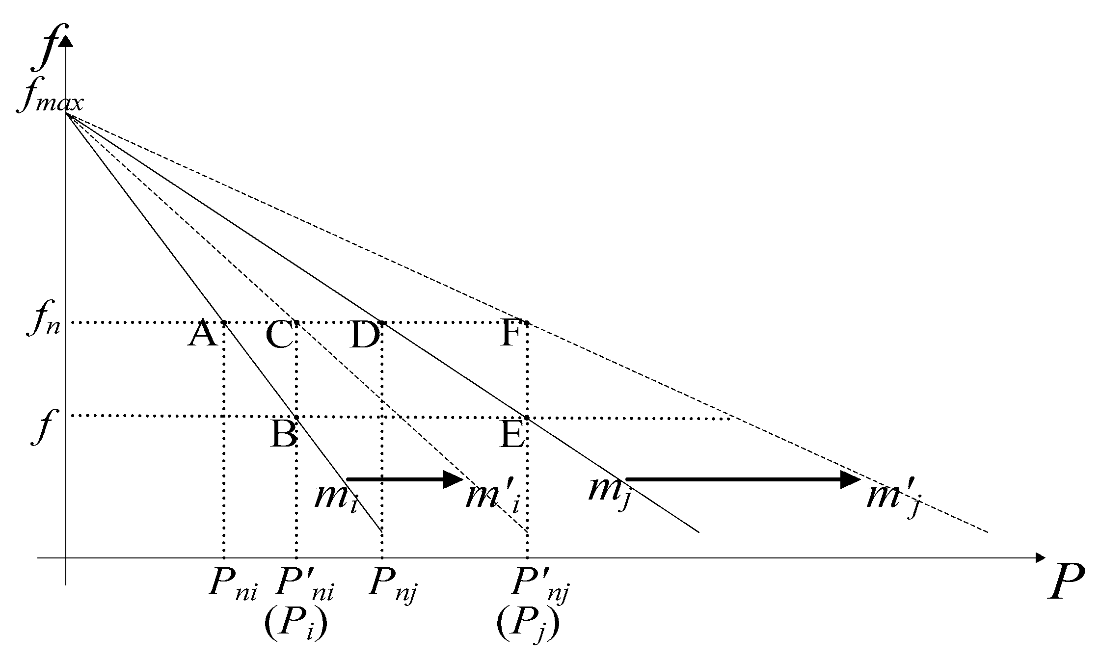
The conventional P-f and Q-E droop characteristics are drawn by the solid lines in Figure 2 and Figure 3, respectively. The output active power is Pni when frequency is fn as shown by point A in Figure 2. The output reactive power is Qni when voltage amplitude is En as shown by point A′ in Figure 3. The operating point moves to point B or point B′ when load varies, and frequency or voltage amplitude deviates from a nominal value. The frequencies of all DGs operated in parallel are equal at steady state (fi = fj = f, i ≠ j). Hence, mi(Pni − Pi) = mj(Pnj − Pj) is obtained in Equation (3) with the P-f droop. mi and mj are chosen to satisfy miPni = mjPnj, then Pi:Pj = (1/mi):(1/mj), so that each DG shares the active power in proportional to power sharing ratio. The power angle θi is generally small, thus, the active power in Equation (2) is approximated as [33]
where Pi is approximated as the delivered active power of DGi into the common bus.
From Equation (4), the voltage magnitude difference (Ei − Ecom) can be expressed as
Assuming that Ei* ≈ Ei and substituting Ei* in Equation (3) into Equation (5) yields
The reactive power sharing error of any two DGs within a microgrid is defined as
From Equation (7), the reactive power sharing error of two DGs includes two terms. The first error term predominantly depends on the voltage magnitude difference (En − Ecom). When niQni = njQnj is satisfied, the first term is zero. The second error term is mainly determined by line resistances and active powers. However, allocating a certain ratio is difficult among actual line impedances, so that PiRi = PjRj is difficult to be realized and the second error term is not identically zero. Thus, the output reactive power among two DGs has a sharing error and accurate reactive power sharing is not accomplished.
3. Improved Droop Control Strategy
In Figure 2, when DGi operating at point B, the output frequency is f, and frequency deviation is Δf (Δf = |fn − f|). This section reconstructs droop control curves to reduce frequency and voltage amplitude deviations. Ignoring the effect of line impedance, DGi operates from point A to B as shown in Figure 2 or point A′ to B′ as shown in Figure 3 when load varies. The output active and reactive power is Pi and Qi, respectively. Let P′ni = Pi and Q′ni = Qi. If (P′ni, fn) be defined as a new nominal operating point, as shown by point C in Figure 2, and an improved P-f droop control curve is reconstructed by connecting the no-load operating point and point C, as the dotted line shown in Figure 2, the droop gain of which is m′i. Similarly, (Q′ni, En) is defined as a new nominal operating point, and an improved Q-E droop control curve is reconstructed as the dotted line containing point C′ shown in Figure 3, the droop gain of which is n′i. The improved droop control formulas are illustrated in Equation (8):
If m′iP′ni = miPni and n′iQ′ni = niQni, then fn + m′iP′ni = fn + miPni = fmax and En + n′iQ′ni = En + niQni = Emax. The improved droop control gains m′i, n′i are illustrated in Equation (9):
At first, we assume that the system operating in point B corresponds to point B′ in Figure 3. Starting the improved droop strategy, DGi moves to point C, corresponding to point C′. The output active power of DGi is Pi, Pi = P′ni. The output reactive power is Qi, Qi = Q′ni. Meanwhile, the frequency and voltage amplitude are restored at nominal values.
Ignoring the effect of line impedance, we assume that two arbitrary DGs operate in parallel, i.e., DGi and DGj, run at nominal points as shown by points A and D in Figure 2, corresponding to points A′ and D′ in Figure 3. When load varies, the two DGs operate at point B (B′) and E (E′) respectively. Let P′ni = Pi, Q′ni = Qi, P′nj = Pj and Q′nj = Qj. If (P′ni, fn) and (Q′ni, En) are defined as new nominal operating points as shown by points C and C′; similarly, (P′nj, fn) and (Q′nj, En) as the new nominal operating points as shown by points F and F′, then the improved droop gains m′i, n′i, m′j and n′j are chosen to satisfy Equation (10):
where m′i, n′i, m′j and n′j are obtained according to Equation (9), such as m′j = (mjPnj)/P′nj and n′j = (njQnj)/Q′nj. The improved P-f droop control curves are reconstructed as dotted lines containing C and F, respectively, shown in Figure 2. Similarly, the improved Q-E droop control curves are reconstructed as dotted lines containing C′ and F′, respectively, shown in Figure 3.
Starting the improved droop strategy, DGi operates from point B (B′) to C (C′), DGj operates from point E (E′) to F (F′). The proportional equation Pi:Pj = P′ni:P′nj = (1/m′i):(1/m′j) = (1/mi):(1/mj) is satisfied, and Q′ni:Q′nj = Qi:Qj = (1/n′i):(1/n′j) = (1/ni):(1/nj). The frequencies and voltage amplitudes are restored at nominal values.
N DG units operated in parallel are extended to analyze the improved droop control strategy when ignoring the effect of line impedance. Let P′ni = Pi and Q′ni = Qi, i = 1, 2, …, N. m′i and n′i, i = 1, 2, …, N, are chosen to satisfy Equation (11):
where m′i, n′i are obtained according to Equation (9). The power sharing ratio satisfies Equation (12):
The power sharing ratio among DGs is generally given by the tertiary control level; i.e., (1/m1):(1/m2):…:(1/mN) and (1/n1):(1/n2):…:(1/nN) are given in advance. The initial values of mi, ni, are also given. To calculate m′i and n′i, P′ni and Q′ni should be obtained. The process of obtaining global load information by all DCrs is elaborated in Section 4. If the global load is expressed as Pload + jQload, then it is shared by all DGs, i.e., Pload = P′n1 + P′n2 + … + P′nN, Qload = Q′n1 + Q′n2 + … + Q′nN. The ith DCr (DCri) calculates the active and reactive power that DGi shares as follows:
where GPi and GQi are power sharing coefficients of DGi, 0 < GPi < 1, and 0 < GQi < 1. DCri calculates P′ni and Q′ni according to Equation (13), then substituting them into Equation (9) to obtain m′i and n′i. Finally, Equation (8) is constructed. The active power sharing ratio is (1/m1):(1/m2):…:(1/mN). Similarly, Q1:Q2:…:QN = (1/n1):(1/n2):…:(1/nN). Meanwhile, f1* = f2* =…= fN* = fn, and E1* = E2* =…= EN* = En. When load varies, DCr obtains new Pload and Qload. Then, P′ni and Q′ni are recalculated. m′i and n′i are obtained and droop control curves are reconstructed. The methods for calculating the variation of droop gains have been given in [34] and the relevant conclusions of eigenvalue analysis have existed, so it is not covered here. Thus, accurate power sharing is always realized, and voltage amplitude and frequency are always kept at nominal values.
The above analysis results are obtained without considering the effect of line impedance. When considering line impedance, the voltage drops across different line impedances are not equal, resulting in the output voltages also not being equal. Thus, the target of reactive power sharing in Equation (12) is difficult to realize.
4. Distributed Secondary Power Optimization Control Based on a Consensus Algorithm
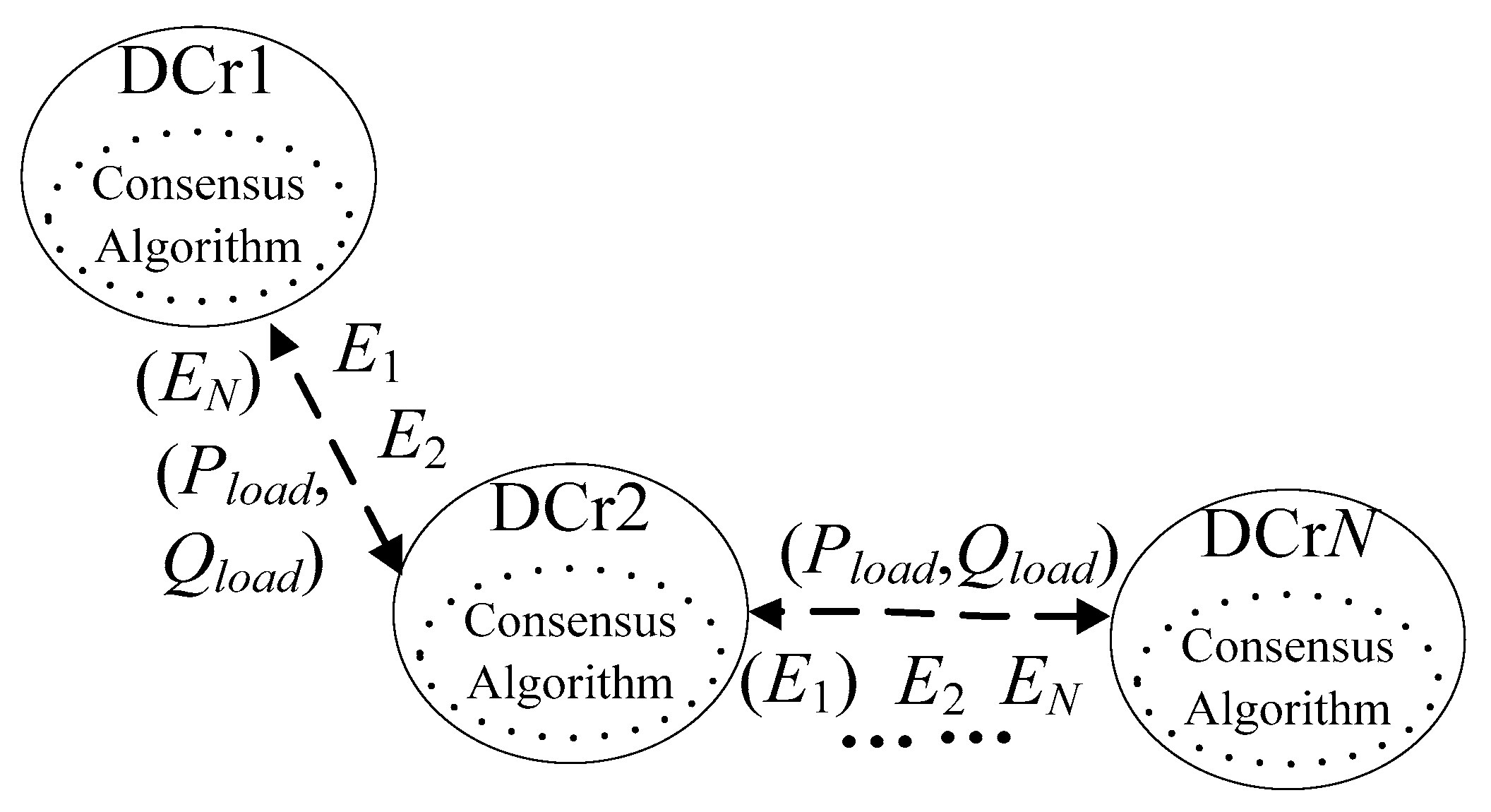
To eliminate the effect of line impedance, a distributed secondary power optimization control is added to the improved Q-E droop control in this section. The average system voltage is obtained by using a discrete consensus algorithm via a distributed sparse communication network which is composed of all DCrs. The simplified distributed sparse communication network is shown in Figure 4. Each DCr is regarded as a node and each node can exchange voltage or load information with neighboring nodes (referring to other nodes that exchange with the node as the neighboring nodes). Two arbitrary nodes exchange information in a bidirectional way. Since an LCr merely transfers load information to the neighboring DCrs in a unidirectional way, as shown in Figure 5 or Figure 6, and do not participate in exchanging voltage information, the distributed sparse communication network does not include LCrs. In Figure 4, DCr2 obtains status information from DCr1 and DCrN by exchanging information with them. Meanwhile, DCr2 can also transfer the status information of DCrN to DCr1; thus, DCr1 obtains the status information of DCrN indirectly. Finally, any status information is obtained by all nodes, e.g., LCr1 transfers the local load information (load1:Pload1 + jQload1) to DCr1 in Figure 6. DCr1 transfers the information of load1 to DCr2, and DCr2 transfers them to DCr3, then all DCrs obtain the information of load1. Similarly, all DCrs can obtain the information of load2 and load3. Then, each DCr obtains the global load information by adding all local load information.
4.1. Discrete Consensus Algorithm
With the feature of simple convergence conditions and fast convergence rate [35,36,37,38], the first order discrete consensus algorithm is used to obtain average system voltage. In Figure 4, the state variables of DCri (i = 1, 2, …, N) is expressed as xi. When the state variables of all nodes are equal or the state variable error is less than the given accuracy, the system reaches consensus convergence by using consensus algorithm. The first-order continuous consensus algorithm is expressed as:
where ui(t) is the input variable of node i and expressed as follows:
where aij is the coefficient for information exchanged between nodes i and j. If nodes i and j are connected through a distribution line, 0 < aij < 1; otherwise, aij = 0. Ni is the indexes of nodes that are connected to node i [36]. This system can concisely be expressed as follows:
where X is the system state variable vector composed of xi. LN is N × N order Laplacian matrix and determined by network topology. The actual system is usually a discrete control system; hence, the first-order discrete consensus algorithm is introduced to analyze system dynamic characteristics.
Equation (17) is expressed in matrix form:
where dij is the element of matrix D. If all elements of matrix D are nonnegative and the sums of each row and column are all ones i.e., D*e = e and DT*e = e, with e = [1, 1, …, 1]T, then D is called the doubly stochastic matrix [37], and the system would reach consensus convergence at the average value of state variables, i.e.,
where X0 is the system initial state variable vector.
An improved Metropolis method was proposed in [38] to construct D, which is expressed in Equation (20), where max(ni, nj) is the maximum number of neighbors among node i and its neighboring nodes. If convergence accuracy ε is given, then Equation (21) expresses iterations.
where λ2 is the second largest eigenvalue of D. However, λ2 may vary with the change of network structure. The accurate value of K is hard to be obtained by applying Equation (21). If the state error of the kth iteration is less than ε, i.e., Equation (22) is satisfied, it can be concluded that a consensus convergence has been reached.
4.2. Distributed Secondary Power Optimization Control Based on a Discrete Consensus Algorithm
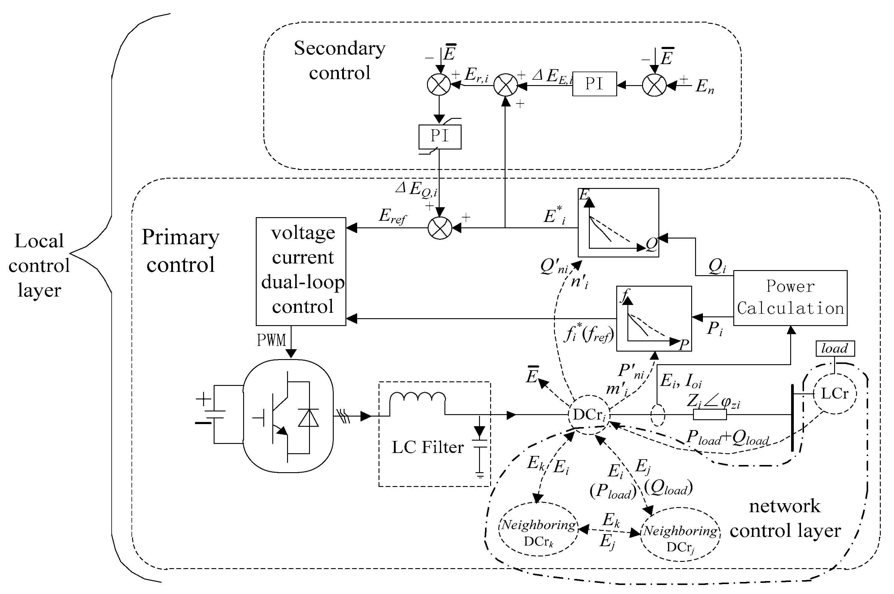
The structure of distributed secondary power optimization control based on improved droop control strategy is illustrated in Figure 5, which contains a local control layer and network control layer. The local control layer consists of primary control and secondary control. Primary control contains an inverter, output filter, power calculation block, the improved droop control block, voltage and current dual-loop control block, and a DC microsource. Secondary control is added to the improved Q-E droop control to optimize reactive power. The network control layer contains DCr and LCr, and is used for transferring load information and exchanging voltage information, meanwhile, using a consensus algorithm to calculate average system voltage, as shown in the dotted line area. Since the frequency is restored at fn and not affected by line impedance, the proposed control strategy in Figure 5 merely needs the reactive power secondary control to optimize reactive power sharing, and the secondary frequency control is no longer needed compared to [26,32]. Meanwhile, output voltage amplitude deviations are further reduced via secondary control, which is illustrated in this section and the simulation results of Section 5.1.
The flow chart of first order discrete consensus algorithm is illustrated in Figure 7. Setting a synchronous sampling clock and its sampling period is Ts. Let t = kTs; each LCr extracts local load information and transfers them to the neighboring DCrs when k = 0. Each DCr extracts voltage information driven by the clock signal and puts them in the local state variable (xi[0]), then exchanges voltage information with neighboring DCrs. Meanwhile, each DCr exchanges local load information with neighboring DCrs and calculates the global load information, then puts them in Pload[0] and Qload[0]. m′i, n′i, P′ni and Q′ni are calculated, respectively. At the next clock signal, xi[k + 1] is calculated by using Equation (16), and the state error of the kth iteration is obtained according to Equation (21). If the state error is greater than or equal to ε, then the iteration repeats. Otherwise, the outputting consensus convergence results are taken to be the average system voltage, i.e., and resetting k = 0. When the next clock signal arrives, each DCr obtains load information and judges Pload[k] with Pload[k − 1]. If Pload[k] = Pload[k − 1], each DCr keeps the m′i and P′ni of the last clock signal; otherwise, they recalculate m′i and P′ni. Similarly, they judge Qload[k] with Qload[k − 1] and recalculate n′i and Q′ni when Qload[k] is not equal to Qload[k − 1].
We assume that the output voltage amplitudes of all DGs are equal at steady state, i.e., E1 = E2 = … = EN = , According to Equation (8),
Ei[k] is the output voltage of DCri at kth iteration, xi[0] = Ei,0. If Equation (22) is satisfied, Ei[k] is set to be applied in DGi, i.e., = Ei[k]. The values of (n′iQ′ni + En − ) are equal for all DGs, then n′iQi are also equal. Hence, the output reactive power is not affected by line impedance, and the relationships of reactive power sharing in Equations (11) and (12) are satisfied. To satisfy the prerequisites of Ei = , i = 1, 2, …, N, (En + n′iQ′ni − n′iQi) is regulated via a Proportional and Integral (PI) controller:
where ΔEQ,i is the regulating variable of reactive power control, kPQ and kIQ are proportional and integral gains of the reactive power PI controller. Substituting Q-E droop control formula in Equation (8) into Equation (24) yields
To make Ei equals to , the reference voltage of DGi is regulated by adding ΔEQ,i to E*i. Due to the effect of line impedance, the average system voltage has a voltage drop even if the improved Q-E droop control is adopted. To keep at En, regulating via a voltage PI controller:
where kPE and kIE are proportional and integral gains of the voltage PI controller. Both the reactive power PI controller and voltage PI controller regulate the reference voltage of Q-E droop control to realize the control target. Merging Equations (25) and (26) yields
where Er,i = E*i + ΔEE,i.
5. Simulation Results
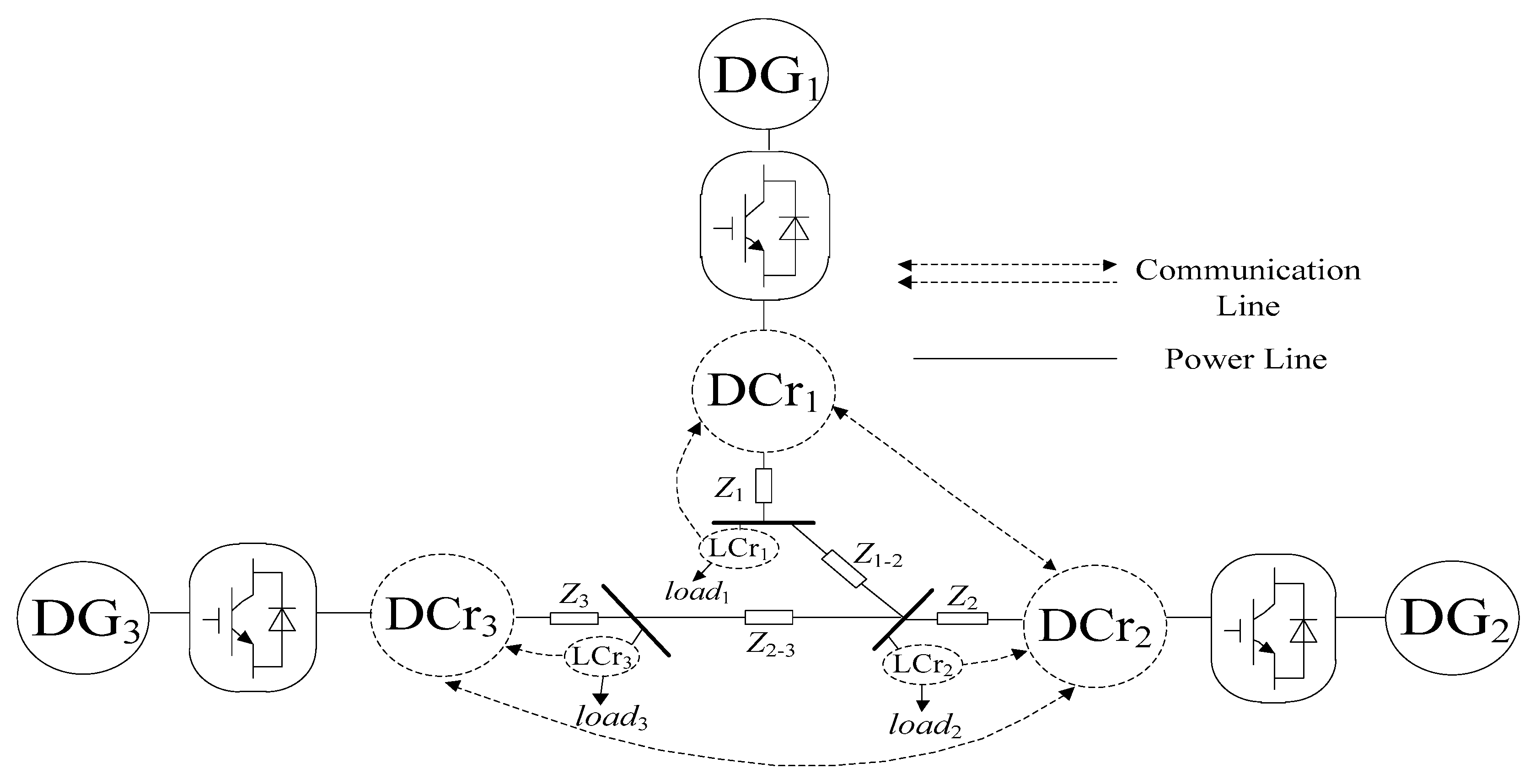
A low-voltage microgrid with three DGs is built based on Matlab R2014a/Simulink, which is shown in Figure 6. Zi(i = 1,2,3) represents the line impedance between DGi and PCC. Zi-j(i, j = 1, 2, 3, i ≠ j) represents the line impedance among different common buses. The initial parameters are shown in Table 1. rf, Lf, and Cf of LC filter are 0.1 Ω, 1.35 mH and 50 μF, respectively. Both the active and reactive power sharing ratio are 3:2:2, i.e., Pn1:Pn2:Pn3 = Qn1:Qn2:Qn3 = 3:2:2. The matrix D is constructed according to Equation (20) and is expressed in Equation (28). fn = 50 Hz and En = 311 V. The system stability is affected by the sampling period [38]. To improve system stability, the sampling period is set to be 0.5 ms in this paper, i.e., Ts = 0.5 ms.
5.1. Case A: Disturbance Analysis
This simulation can be divided into four stages:
- Stage 1 (0–1 s):
- The conventional droop control shown in Equation (3) is used to control the 3 DGs in Figure 6. Load 1 and Load 2 are connected to the system at t = 0 s.
- Stage 2 (1–2 s):
- The improved droop control shown in Equation (8) is used to control the 3 DGs at t = 1 s.
- Stage 3 (2–3 s):
- The secondary power optimization control is added to the improved Q-E droop control to optimize reactive power and regulate voltage amplitude at t = 2 s.
- Stage 4 (3–4 s):
- Load 3 is connected to the system at t = 3 s.
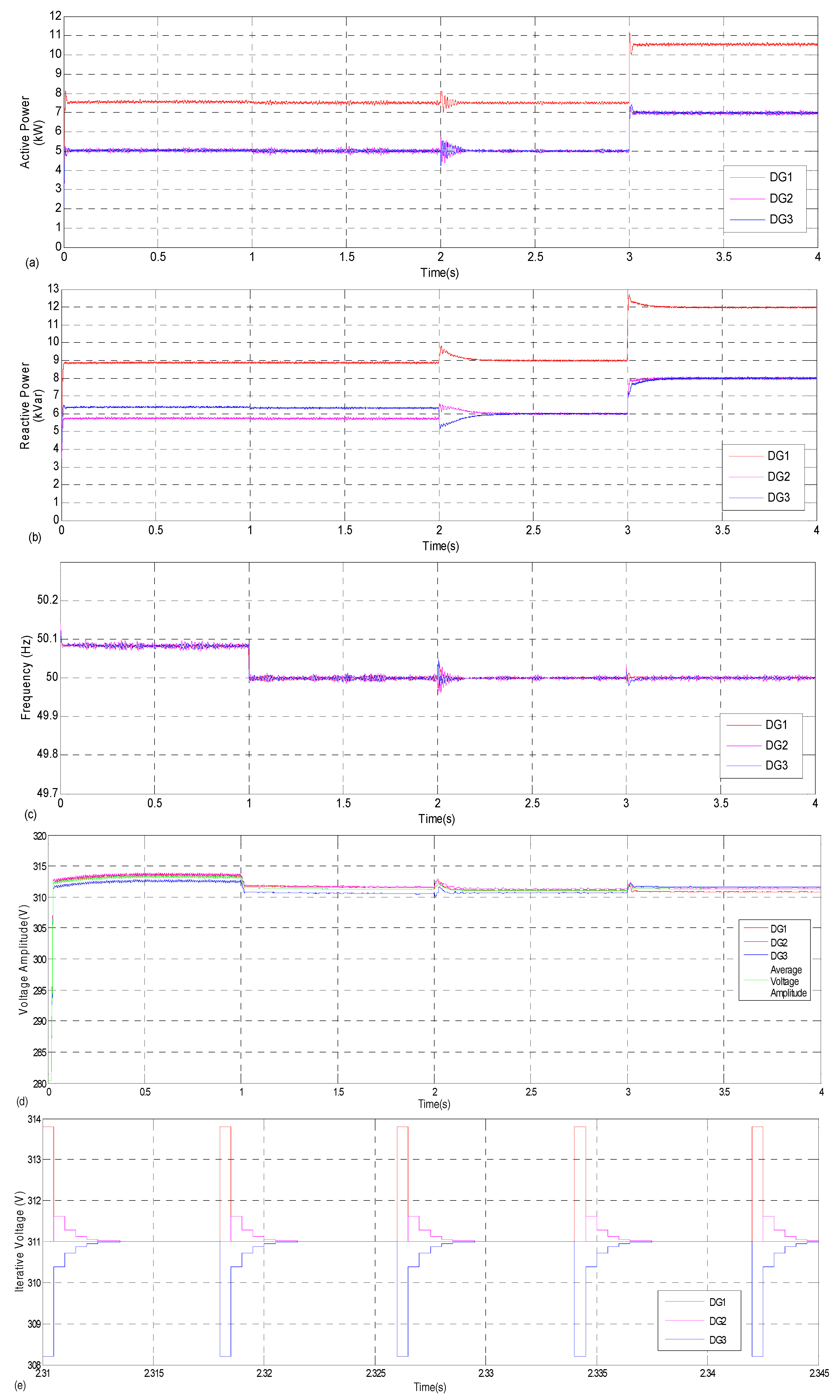
The state error accuracy ε is set to be 0.01. The simulation results are shown in Figure 8. The active and reactive power are illustrated in Figure 8a,b, respectively. The output frequency and voltage amplitude are illustrated in Figure 8c,d, respectively. Figure 8e shows the kth iterative voltage of DCri in the process of discrete consensus algorithm, i.e., Ei[k]. During stage 1, the frequencies of all DGs are equal and deviating from 50 Hz as seen from Figure 8c. The active powers are 7.49 kW, 5.01 kW, 5 kW, respectively, i.e., P1:P2:P3 = 3:2:2, as seen from Figure 8a. The reactive power cannot be shared in proportional to 3:2:2 and Q2 ≠ Q3 as seen from Figure 8b. Figure 8d illustrates the output voltages of DG1, DG2 and DG3 are 313.6 V, 313.7 V and 312.4 V, respectively, and the average system voltage is 313.23 V. Both output voltages and average system voltage deviate from 311 V.
Starting the improved droop control at t = 1 s. During stage 2, the voltage frequencies of all DGs are restored to be 50 Hz, shown in Figure 8c. The active powers are 7.5 kW, 5 kW, 5 kW, respectively. The output voltages are 311.3 V, 311.3 V and 310.6 V, respectively, and = 311.07 V. Thus, output voltage amplitude deviations are reduced, but accurate reactive power sharing is still not realized. Figure 8b shows the reactive power sharing ratio is not 3:2:2 and Q2 ≠ Q3.
The secondary control is added to the improved Q-E droop control at t = 2 s. During stage 3, the reactive powers are 8.97 kVar, 5.97 kVar, 5.98 kVar shown in Figure 8b, and the sharing ratio is 3:2:2. Figure 8d shows the voltages are 311.12 V, 311.1 V and 310.78 V, respectively, and = 311 V. It reveals that accurate reactive power sharing is achieved, and voltage amplitude deviations are further reduced compared with Stage 2. Figure 8e shows that the three output voltages of DCrs are equal to 311 V after several iterative calculations. Load 3 is connected to the system at t = 3 s. At first, the active and reactive power sharing accuracies are decreased. The system reaches a steady state after a short time adjustment. During Stage 4, the frequencies of all DGs are 50 Hz. Figure 8d shows the voltages are 310.7 V, 311.15 V and 311.15 V, respectively, and =311 V. Figure 8a shows P1, P2, P3 are 10.49 kW, 6.99 kW, 6.99 kW, and the sharing ratio is 3:2:2. Figure 8b shows Q1, Q2, Q3 are 11.96 kVar, 7.97 kVar, 7.98 kVar, and the sharing ratio is also 3:2:2.
Figure 8 shows that the proposed control strategy, combining the improved droop control with distributed secondary power optimization control, can share active and reactive power in proportion to the power sharing ratio. Meanwhile, the frequencies of all DGs and average system voltage are kept at nominal values, and the output voltage amplitude deviations are all reduced.
5.2. Case B: Variations of Line Impedance
Four sets of scenario simulations with different line impedances are designed according to the microgrid model shown in Figure 6. Loads 1 and 2 are connected to the system and the reactive power sharing ratio is 3:2:2. The line impedances of all groups are shown in Table 2. Group 1 uses the conventional droop control shown in Equation (3) to regulate all DGs. Groups 2, 3 and 4 use the improved droop control combined with secondary control to regulate all DGs. The reactive powers, output voltages and the corresponding deviations are shown in Table 3. The average voltage deviation is the deviation between average system voltage and 311 V. The average reactive power deviation is designed as
Table 3 reveals that the reactive power sharing ratio is not 3:2:2 in Group 1; meanwhile, both average voltage deviation and average reactive power deviation are larger than the simulation results in Groups 2, 3 and 4. The eQ of Groups 2, 3 and 4 are 0.204%, 0.185% and 0.148%, respectively. The average voltage deviations of Groups of 2, 3 and 4 are 0 V, 0.033 V and 0 V, respectively. The line impedances in Group 1 and Group 2 are equal, and the two groups′ simulation results reveal that the control strategy proposed in this paper can share reactive power accurately in proportional to the sharing ratio; meanwhile, the average system voltage is kept at nominal value and all output voltage deviations are reduced. Groups 2, 3 and 4 reveal that the accurate reactive power sharing is not affected by line impedance variations and the average system voltage can be kept at nominal value under different line impedances.
5.3. Case C: Influence of Different Convergence Accuracies
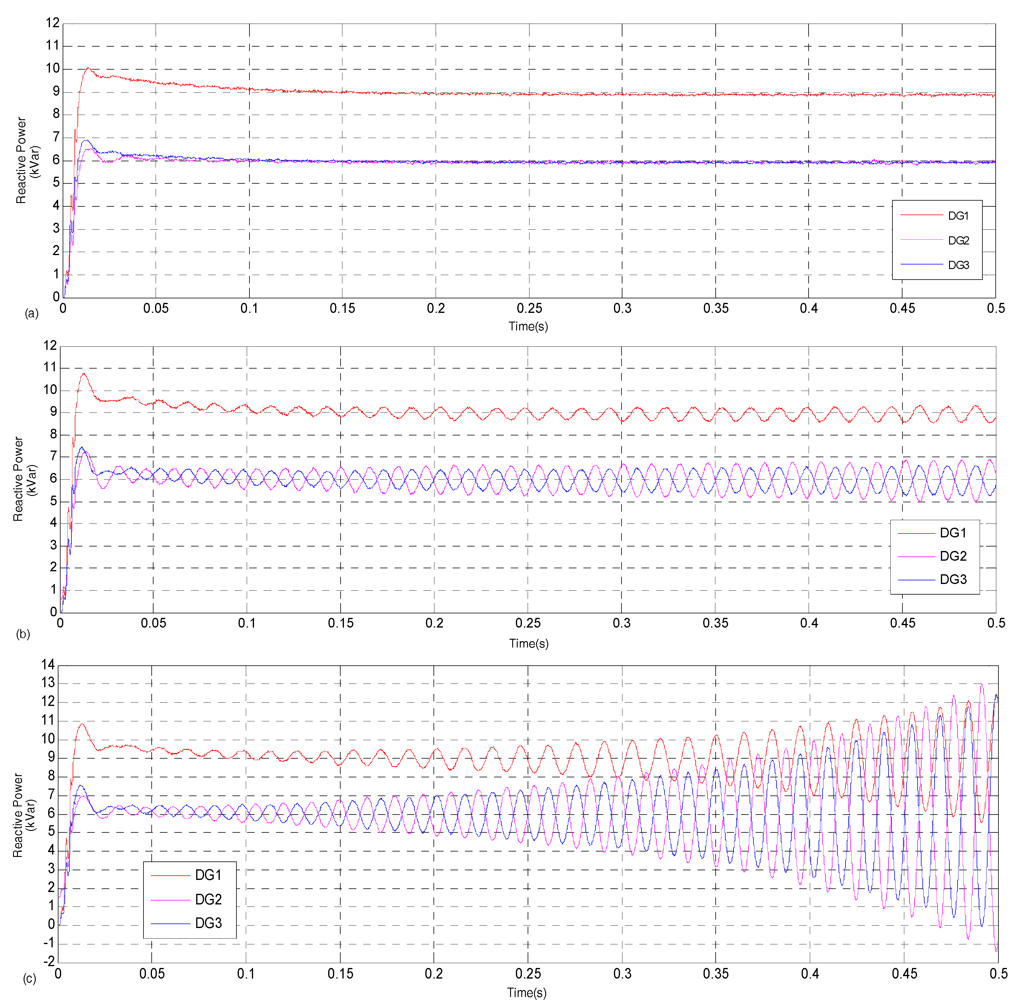
Equation (21) shows that the iterations vary when convergence accuracies (ε) change. The higher the accuracy or the smaller the ε, the more iterations. Thus, it takes a long time to calculate average value. On the contrary, the lower the accuracy, the fewer iterations. Three sets of scenario simulations with the effect of different ε are designed. The ε are 0.1, 0.01 and 0.001, respectively. The reactive power sharing ratio is 3:2:2. Load 1 and Load 2 are connected to the system at t = 0 s. Load 3 is connected to the system at t = 0.5 s. The different output voltages of DCri via consensus algorithm and the corresponding voltage convergence deviations are shown in Table 4. The voltage convergence deviation is designed as:
where Ei is the output voltage of DCri via consensus algorithm, Eave is the average output iterative voltage.
From Table 4, the eE with ε is 0.1 is larger than the values of eE with ε are 0.01 and 0.001. The eE is 0.0337 × 10⁻³ when ε is 0.01, which is larger than the eE with ε is 0.001. Table 4 reveals that the smaller the ε, the smaller the voltage convergence deviation. From Figure 9a, Q2 is not equal to Q3 when ε is 0.1. This reveals that accurate reactive power sharing is not realized when the convergence accuracy is low. From Figure 9b,c, the target of accurate reactive power sharing in proportional to 3:2:2 is realized when ε is 0.01 or 0.001. Comparing Figure 9b,c the adjustment process with ε is 0.01 is more smooth when the process with ε is 0.001 at t = 0.5 s. The adjustment process appears to overshoot at t = 0.5 s when ε is 0.001. This is due to a high convergence accuracy requiring more iterations, thus prolonging iteration time. It takes a long time to update the output iterative voltage, resulting in the output iterative voltage cannot be timely used by secondary Q-E droop control, thus the transient performance is reduced.
From the above analysis, the smaller the ε is given, the more iterations and the longer iteration time are needed. Although the convergence accuracy is improved, the transient performance is reduced. On the contrary, the target of accurate reactive power sharing cannot be realized when the convergence accuracy is too low. Therefore, both the accurate reactive power sharing ratio and transient performance are considered to set the ε reasonably. The ε is set to be 0.01 in Section 5.1 and Section 5.2 to guarantee accurate reactive power sharing and smooth transient performance.
5.4. Case D: Influence of Communication Delay
Section 4 shows that each DCr updates voltage or load information every other sampling period (Ts). If a DCr obtains load information exceeding the time of a sampling period, then the load information cannot be timely used by a DCr. This section discusses the influence of different time delays in communication system. If the communication delay is τ, i.e., a DCr or LCr sends information after τ milliseconds of the arrival of the clock signal, then the interval time that a DCr updates information or a LCr transfers load information to the neighboring DCrs is Δt (Δt = Ts + τ). The τ are 0.05 ms, 0.25 ms and 0.5 ms, respectively. The reactive power sharing ratio is 3:2:2. ε is 0.01. Load 1 and Load 2 are connected to the system at t = 0 s. Different simulation results are shown in Figure 10.
Figure 10a shows that the starting process appears to overshoot when τ is 0.05 ms, which is similar to Figure 9c. This is due to the fact that relevant information, such as average system voltage, cannot be utilized in a timely fashion as a result of communication delay. Figure 10b shows that the output reactive powers appear largely fluctuations when τ is 0.25 ms. Figure 10c shows that the simulation results are oscillatory and the system is unstable when τ is 0.5 ms. The simulation results reveal that the dynamic output performance of the microgrid would be deteriorated when a delay exists in the communication system, and that the excessive communication delay would result in system instability.
6. Conclusions
A control strategy combining an improved droop control which can regulate droop gains with distributed secondary power optimization control is proposed. The improved P-f droop control can always keep frequency at a nominal value when load varies without secondary frequency control; meanwhile, sharing the active power in proportion to the power sharing ratio. The distributed secondary reactive power optimization control based on a consensus algorithm is added to the improved Q-E droop control. With the control strategy, average system voltage is kept at a nominal value and the output voltage amplitude deviations of all DGs are reduced to a large extent. Meanwhile, the target of accurate reactive power sharing in proportion to the power sharing ratio is realized. The reasonable value of the convergence accuracy (ε) used in the consensus algorithm is determined by simulation to satisfy both accurate reactive power sharing and transient performance. The simulation results also reveal that accurate reactive power sharing is not affected by line impedance variations and that excessive communication delay would result in system instability. The control strategy based on a distributed sparse communication network does not need MGCC, which gives the strategy a good reliability. The simulation results have also verified its effectiveness.
Acknowledgments
This work was supported by National High Technology Research and Development Program of China (No. 2015AA050104) and supported by the Key R&R Program of Jiangsu province (BE2015012-1).
Author Contributions
Demin Li conceived the main idea, performed simulations, and wrote the manuscript. Zaijun Wu and Bo Zhao contributed to developing the ideas in this research. Xuesong Zhang and Leiqi Zhang thoroughly revised the paper.
Conflicts of Interest
The authors declare no conflict of interest.
References
- Wang, H.; Huang, J. Joint Investment and Operation of Microgrid. IEEE Trans. Smart Grid 2017, 8, 833–845. [Google Scholar] [CrossRef]
- Golsorkhi, M.S.; Lu, D.D.C. A control method for inverter-based islanded microgrids based on V-I droop characteristics. IEEE Trans. Power Deliv. 2015, 30, 1196–1204. [Google Scholar] [CrossRef]
- Ahn, C.; Peng, H. Decentralized and real-time power dispatch control for an islanded microgrid supported by distributed power sources. Energies 2013, 6, 6439–6454. [Google Scholar] [CrossRef]
- Katiraei, F.; Iravani, M.R.; Lehn, P.W. Microgrid autonomous operation during and subsequent to islanding process. IEEE Trans. Power Deliv. 2005, 20, 248–257. [Google Scholar] [CrossRef]
- Yu, Z.; Ai, Q.; He, X.; Piao, L. Adaptive droop control for microgrids based on the synergetic control of multi-agent systems. Energies 2016, 9, 1057. [Google Scholar] [CrossRef]
- Guerrero, J.M.; Vasquez, J.C.; Matas, J.; Vicuna, L.G.D.; Castilla, M. Hierarchical control of droop-controlled AC and DC microgrids—A General Approach Toward Standardization. IEEE Trans. Ind. Electron. 2011, 58, 158–172. [Google Scholar] [CrossRef]
- Bidram, A.; Davoudi, A. Hierarchical structure of microgrids control system. IEEE Trans. Smart Grid 2012, 3, 1963–1976. [Google Scholar] [CrossRef]
- Parhizi, S.; Lotfi, H.; Khodaei, A.; Bahramirad, S. State of the art in research on microgrids: A review. IEEE Access 2015, 3, 890–925. [Google Scholar] [CrossRef]
- Lu, X.; Guerrero, J.M.; Sun, K.; Vasquez, J.C.; Teodorescu, R.; Huang, L. Hierarchical control of parallel AC-DC converter interfaces for hybrid microgrids. IEEE Trans. Smart Grid 2014, 5, 683–692. [Google Scholar] [CrossRef]
- Patterson, M.; Macia, N.F.; Kannan, A.M. Hybrid microgrid model based on solar photovoltaic battery fuel cell system for intermittent load applications. IEEE Trans. Energy Convers. 2015, 30, 359–366. [Google Scholar] [CrossRef]
- Dragicevic, T.; Guerrero, J.M.; Vasquez, J.C.; Škrlec, D. Supervisory control of an adaptive-droop regulated dc Microgrid with battery management capability. IEEE Trans. Ind. Electron. 2014, 29, 695–706. [Google Scholar] [CrossRef]
- Egwebe, A.M.; Fazeli, M.; Igic, P.; Holland, P.M. Implementation and stability study of dynamic droop in islanded microgrids. IEEE Trans. Energy Convers. 2016, 31, 821–832. [Google Scholar] [CrossRef]
- Guo, F.; Wen, C.; Mao, J.; Song, Y. Distributed secondary voltage and frequency restoration control of droop-controlled inverter-based microgrids. IEEE Trans. Ind. Electron. 2015, 62, 4355–4364. [Google Scholar] [CrossRef]
- Guerrero, J.M.; Matas, J.; de Vicuña, L.G. Decentralized control for parallel operation of distributed generation inverters using resistive output impedance. IEEE Trans. Ind. Electron. 2007, 54, 994–1004. [Google Scholar] [CrossRef]
- Gu, W.; Liu, W.; Wu, Z.; Zhao, B.; Chen, W. Cooperative control to enhance the frequency stability of islanded microgrids with DFIG-SMES. Energies 2013, 6, 3951–3971. [Google Scholar] [CrossRef]
- Tuladhar, A.; Jin, H.; Unger, T.; Mauch, K. Control of parallel inverters in distributed AC power systems with consideration of line impedance effect. IEEE Trans. Ind. Appl. 2000, 36, 131–138. [Google Scholar] [CrossRef]
- Li, Y.; Kao, C.-N. An accurate power control strategy for power-electronics-interfaced distributed generation units operating in a low-voltage multibus microgrid. IEEE Trans. Power Electron. 2009, 24, 2977–2988. [Google Scholar]
- Guerrero, J.M.; Vicuna, L.G.D.; Matas, J.; Castilla, M.; Miret, J. Out impedance design of parallel-connected UPS inverters with wireless load-sharing control. IEEE Trans. Ind. Electron. 2005, 52, 1126–1135. [Google Scholar] [CrossRef]
- He, J.; Li, Y. Analysis, design, and implementation of virtual impedance for power electronics interfaced distributed generation. IEEE Trans. Ind. Appl. 2011, 47, 2525–2538. [Google Scholar] [CrossRef]
- Zhu, Y.; Zhuo, F.; Wang, F.; Liu, B.; Gou, R.; Zhao, Y. A virtual impedance optimization method for reactive power sharing in networked microgrid. IEEE Trans. Power Electron. 2016, 31, 2890–2904. [Google Scholar] [CrossRef]
- Majumder, R.; Ledwich, G.; Ghosh, A. Droop control of converter-interfaced microsources in rural distributed generation. IEEE Trans. Power Deliv. 2010, 25, 2768–2778. [Google Scholar] [CrossRef] [Green Version]
- Hajizadeh, A.; Golkar, M.A. Intelligent power management strategy of hybrid distributed generation system. Int. J. Electr. Power Energy Syst. 2007, 29, 783–795. [Google Scholar] [CrossRef]
- Wang, C.; Yang, X.; Wu, Z.; Che, Y.; Guo, L.; Zhang, S.; Liu, Y. A Highly integrated and reconfigurable microgrid testbed with hybrid distributed energy sources. IEEE Trans. Smart Grid 2016, 7, 451–459. [Google Scholar] [CrossRef]
- Yao, W.; Chen, M.; Matas, J.; Guerrero, J.M.; Qian, Z. Design and analysis of the droop control method for parallel inverters considering the impact of the complex impedance on the power sharing. IEEE Trans. Ind. Electron. 2011, 58, 576–588. [Google Scholar] [CrossRef]
- Ahn, S.J.; Nam, S.R.; Choi, J.H.; Moon, S.I. Power scheduling of distributed generators for economic and stable operation of a microgrid. IEEE Trans. Smart Grid 2013, 4, 398–405. [Google Scholar] [CrossRef]
- Shafiee, Q.; Guerrero, J.M.; Vasquez, J.C. Distributed secondary control for islanded microgrids—A novel approach. IEEE Trans. Power Electron. 2014, 29, 1018–1030. [Google Scholar] [CrossRef]
- Nasirian, V.; Davoudi, A.; Lewis, F.L.; Guerrero, J.M. Distributed adaptive droop control for DC distribution systems. IEEE Trans. Energy Convers. 2014, 29, 944–956. [Google Scholar] [CrossRef]
- Zhong, Q. Robust droop controller for accurate proportional load sharing among inverters operated in parallel. IEEE Trans. Ind. Electron. 2013, 60, 1281–1290. [Google Scholar] [CrossRef]
- Wu, D.; Dragicevic, T.; Vasquez, J.C.; Guerrero, J.M. Secondary coordinated control of islanded microgrids based on consensus algorithms. In Proceedings of the Energy Conversion Congress and Exposition (ECCE), Pittsburgh, PA, USA, 14–18 September 2014; pp. 4290–4297. [Google Scholar]
- Vandoorn, T.L.; Kooning, J.D.M.D.; Vyver, J.V.D.; Vandevelde, L. Three-Phase Primary Control for Unbalance Sharing between Distributed Generation Units in a Microgrid. Energies 2013, 6, 6586–6607. [Google Scholar] [CrossRef] [Green Version]
- Mohamed, Y.; El-Saadany, E.F. Adaptive decentralized droop controller to preserve power sharing stability of paralleled inverters in distributed generation microgrids. IEEE Trans. Power Electron. 2008, 23, 2806–2816. [Google Scholar] [CrossRef]
- Savaghebi, M.; Jalilian, A.; Vasquez, J.C.; Guerrero, J.M. Secondary Control Scheme for Voltage Unbalance Compensation in an Islanded Droop-Controlled Microgrid. IEEE Trans. Smart Grid 2012, 3, 797–807. [Google Scholar] [CrossRef]
- Hou, X.; Sun, Y.; Yuan, W.; Zhong, C. Conventional P-ω/Q-V droop control in highly resistive line of low-voltage converter-based AC microgrid. Energies 2016, 9, 943. [Google Scholar] [CrossRef]
- Hatano, Y.; Mesbahi, M. Agreement over random networks. IEEE Trans. Autom. Control 2005, 50, 1867–1872. [Google Scholar] [CrossRef]
- Pogaku, N.; Prodanovic, M.; Green, T.C. Modeling, Analysis and Testing of Autonomous Operation of an Inverter-Based Microgrid. IEEE Trans. Power Electron. 2007, 22, 613–625. [Google Scholar] [CrossRef]
- Khoo, S.; Xie, L.; Man, Z. Robust Finite-Time Consensus Tracking Algorithm for Multirobot Systems. IEEE/ASME Trans. Mechatron. 2009, 14, 219–228. [Google Scholar] [CrossRef]
- Xu, Y.; Liu, W. Novel multiagent based load restoration algorithm for microgrids. IEEE Trans. Smart Grid 2011, 2, 152–161. [Google Scholar] [CrossRef]
- Zhang, Z.; Chow, M.Y. Convergence analysis of the incremental cost consensus algorithm under different communication network topologies in a smart grid. IEEE Trans. Power Syst. 2012, 27, 1761–1768. [Google Scholar] [CrossRef]
Figure 1.
Equivalent model of many sets of distributed generators connected in parallel.
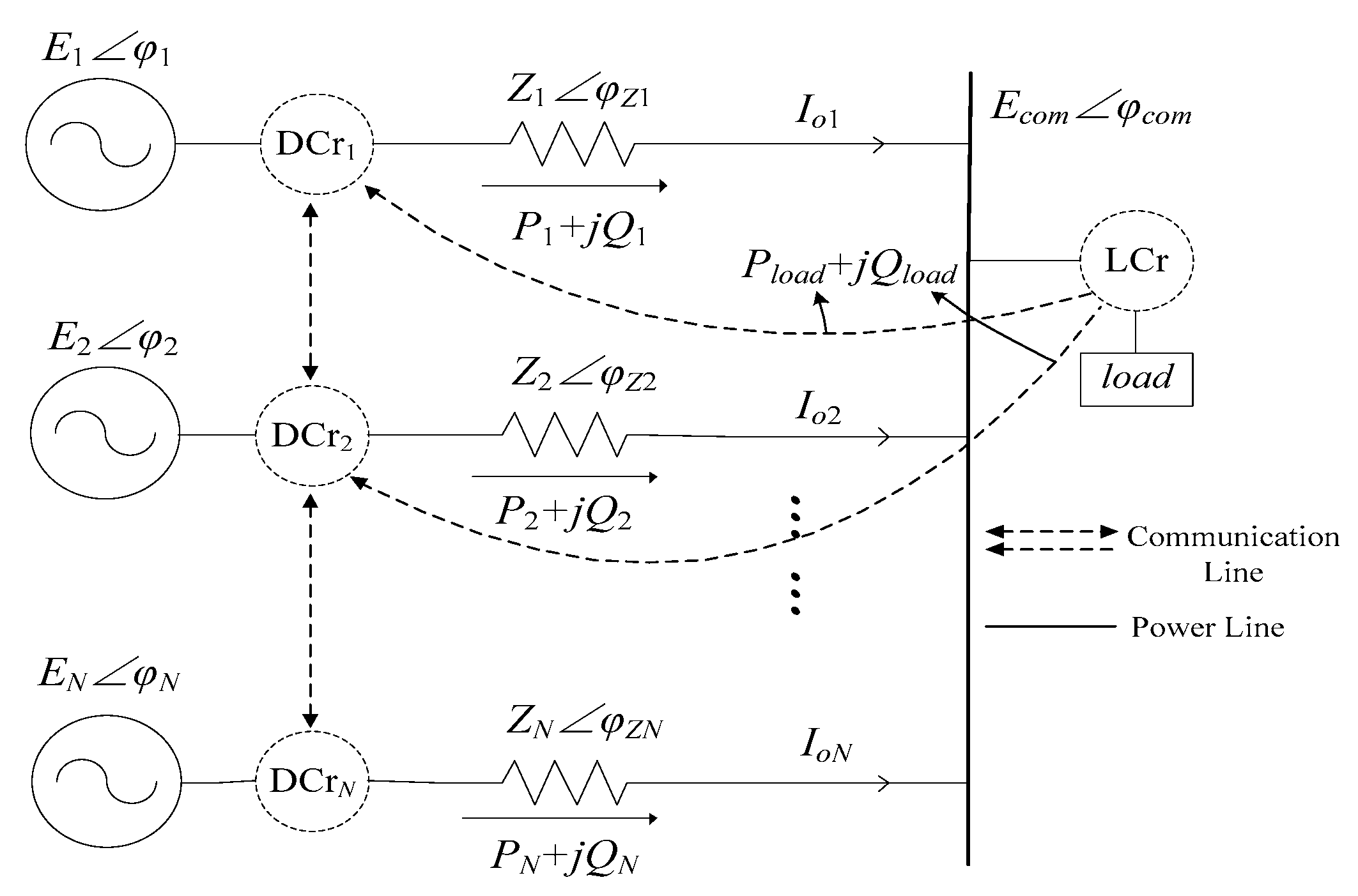
Figure 2.
Conventional and improved P-f droop control characteristics.

Figure 3.
Conventional and improved Q-E droop control characteristics.

Figure 4.
Distributed sparse communication network.

Figure 5.
Structure of distributed secondary power optimization control based on the improved droop control strategy.
Figure 5.
Structure of distributed secondary power optimization control based on the improved droop control strategy.

Figure 6.
Structure of the AC microgrid.

Figure 7.
Flow chart of the discrete consensus algorithm.
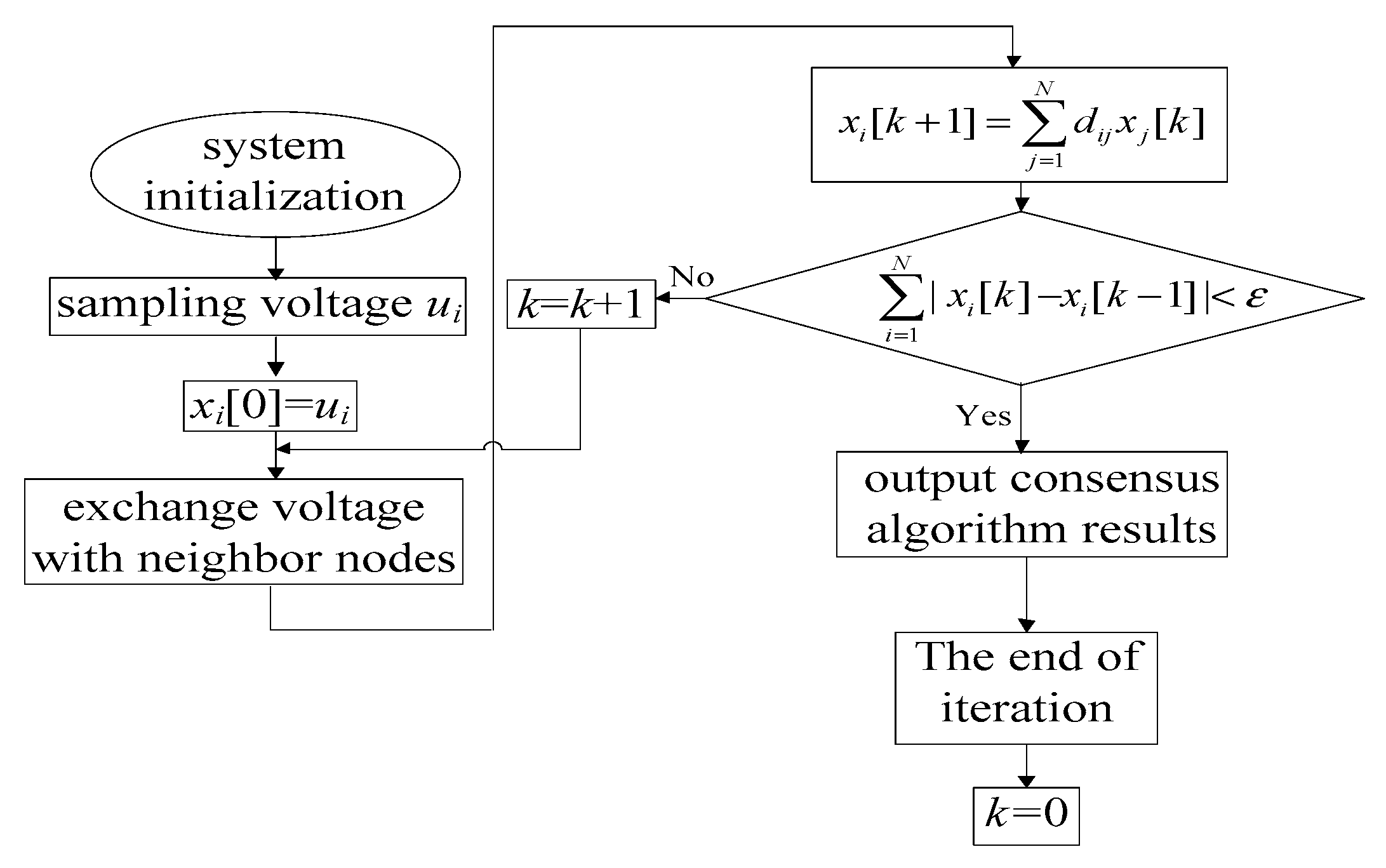
Figure 8.
Simulation results in Case A: (a) active power; (b) reactive power; (c) frequency; (d) output voltage amplitude and average voltage amplitude; and (e) iterative voltage amplitude.
Figure 8.
Simulation results in Case A: (a) active power; (b) reactive power; (c) frequency; (d) output voltage amplitude and average voltage amplitude; and (e) iterative voltage amplitude.

Figure 9.
Simulation results in Case C: (a) reactive power with ε is 0.1; (b) reactive power with ε is 0.01; and (c) reactive power with ε is 0.001.
Figure 9.
Simulation results in Case C: (a) reactive power with ε is 0.1; (b) reactive power with ε is 0.01; and (c) reactive power with ε is 0.001.
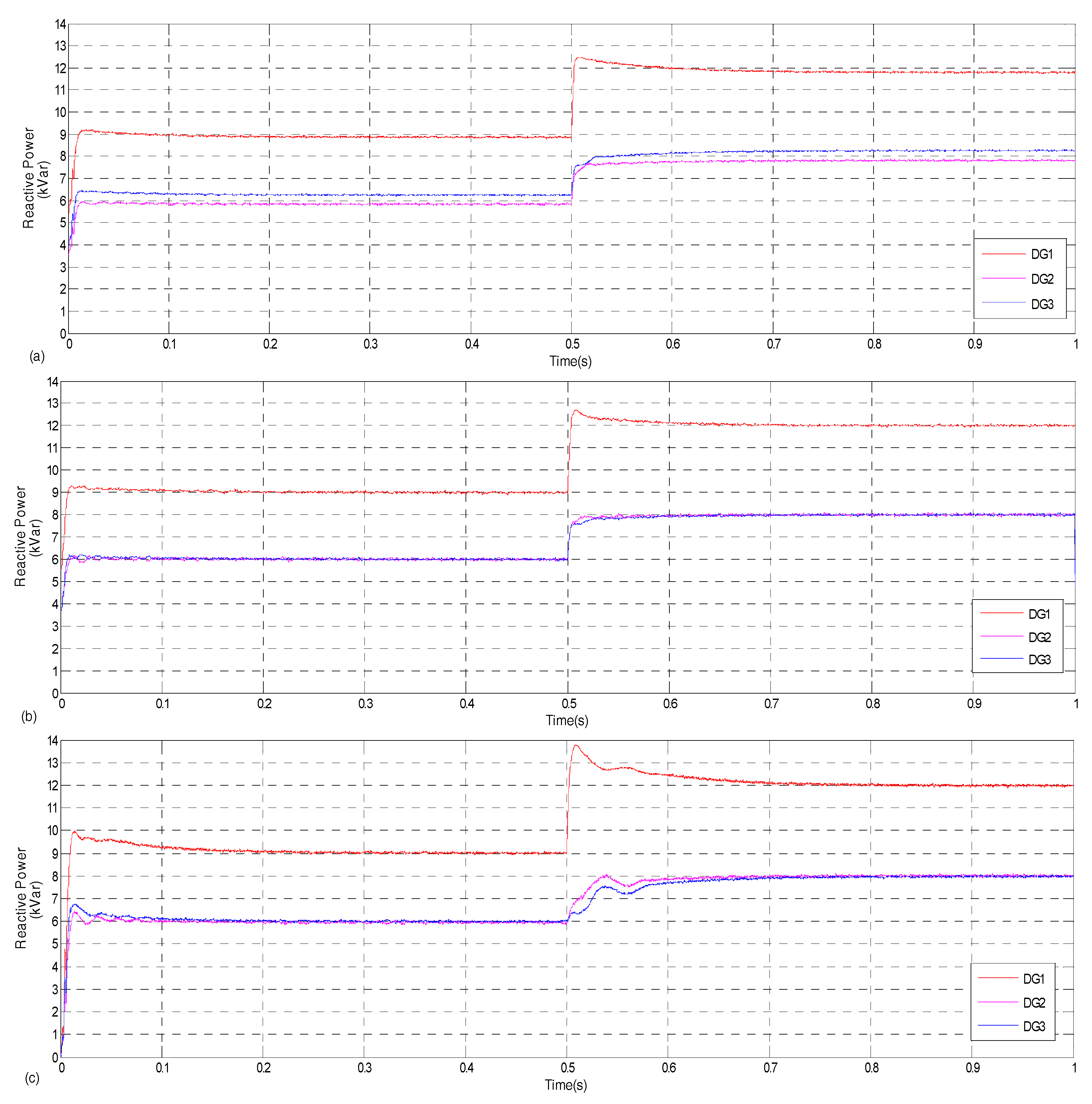
Figure 10.
Simulation results in Case D: (a) reactive power with τ is 0.05ms; (b) reactive power with τ is 0.25ms; and (c) reactive power with τ is 0.5ms.
Figure 10.
Simulation results in Case D: (a) reactive power with τ is 0.05ms; (b) reactive power with τ is 0.25ms; and (c) reactive power with τ is 0.5ms.


Table 1.
Parameters of the model.
| DG | P-f Droop Gain mi,0 (Hz/kW) | Q-E Droop Gain ni,0 (V/kVar) | Rated Active Power Pni,0 (kW) | Rated Reactive Power Qni,0 (kVar) | Load | Values | Line Impedance | Values |
|---|---|---|---|---|---|---|---|---|
| DG1 | 0.0556 | 1.4286 | 9 | 10.5 | Load1/KVA | 9 + j10 | Z1/Ω | 0.2 + j0.031 |
| DG2 | 0.0833 | 2.1429 | 6 | 7 | Load2/KVA | 8.5 + j11 | Z2/Ω | 0.3 + j0.063 |
| Z3/Ω | 0.2 + j0.031 | |||||||
| DG3 | 0.0833 | 2.1429 | 6 | 7 | Load3/KVA | 7 + j7 | Z1-2/Ω | 0.4 + j0.063 |
| Z2-3/Ω | 0.5 + j0.094 |
Table 2.
Parameters of line impedance in different groups.
| Groups | Z1/Ω | Z2/Ω | Z3/Ω | Z1-2/Ω | Z2-3/Ω |
|---|---|---|---|---|---|
| Group 1 | 0.2 + j0.031 | 0.4 + j0.063 | 0.3 + j0.063 | 0.5 + j0.063 | 0.4 + j0.063 |
| Group 2 | 0.2 + j0.031 | 0.4 + j0.063 | 0.3 + j0.031 | 0.5 + j0.063 | 0.4 + j0.063 |
| Group 3 | 0.3 + j0.063 | 0.3 + j0.063 | 0.2 + j0.031 | 0.6 + j0.094 | 0.5 + j0.063 |
| Group 4 | 0.2 + j0.031 | 0.3 + j0.063 | 0.2 + j0.031 | 0.4 + j0.063 | 0.5 + j0.094 |
Table 3.
System steady-state operation results in different groups.
| Groups | Parameters | DG1 | DG2 | DG3 |
|---|---|---|---|---|
| Group 1 | Reactive Power/kVar | 8.86 | 5.61 | 6.37 |
| Voltage/V | 313.1 | 314 | 313.2 | |
| eQ/% | 4.741 | |||
| Average Voltage Deviation/V | 2.433 | |||
| Group 2 | Reactive Power/kVar | 8.99 | 5.98 | 5.99 |
| Voltage/V | 310.5 | 311.2 | 311.3 | |
| eQ/% | 0.204 | |||
| Average Voltage Deviation/V | 0 | |||
| Group 3 | Reactive Power/kVar | 8.98 | 5.99 | 5.99 |
| Voltage/V | 311.7 | 311.1 | 310.3 | |
| eQ/% | 0.185 | |||
| Average Voltage Deviation/V | 0.033 | |||
| Group 4 | Reactive Power/kVar | 8.99 | 5.98 | 6.00 |
| Voltage/V | 310.7 | 311.4 | 310.9 | |
| eQ/% | 0.148 | |||
| Average Voltage Deviation/V | 0 | |||
Table 4.
Convergence results and deviations under different convergence accuracies.
| ε | Ei/V | eE/× 10−3 | ||
|---|---|---|---|---|
| DCr1 | DCr2 | DCr3 | ||
| 0.1 | 311.0752 | 311.1621 | 311.1132 | 0.0970 |
| 0.01 | 310.9923 | 311.0126 | 310.9857 | 0.0337 |
| 0.001 | 310.9931 | 310.9951 | 310.9937 | 0.0024 |
© 2017 by the authors. Licensee MDPI, Basel, Switzerland. This article is an open access article distributed under the terms and conditions of the Creative Commons Attribution (CC BY) license (http://creativecommons.org/licenses/by/4.0/).
Share and Cite
MDPI and ACS Style
Li, D.; Zhao, B.; Wu, Z.; Zhang, X.; Zhang, L. An Improved Droop Control Strategy for Low-Voltage Microgrids Based on Distributed Secondary Power Optimization Control. Energies 2017, 10, 1347. https://doi.org/10.3390/en10091347
AMA Style
Li D, Zhao B, Wu Z, Zhang X, Zhang L. An Improved Droop Control Strategy for Low-Voltage Microgrids Based on Distributed Secondary Power Optimization Control. Energies. 2017; 10(9):1347. https://doi.org/10.3390/en10091347
Chicago/Turabian StyleLi, Demin, Bo Zhao, Zaijun Wu, Xuesong Zhang, and Leiqi Zhang. 2017. "An Improved Droop Control Strategy for Low-Voltage Microgrids Based on Distributed Secondary Power Optimization Control" Energies 10, no. 9: 1347. https://doi.org/10.3390/en10091347
Note that from the first issue of 2016, this journal uses article numbers instead of page numbers. See further details here.