On the Influence of Operational and Control Parameters in Thermal Response Testing of Borehole Heat Exchangers

 , , ,
, , , 
Abstract
:1. Introduction
2. Method
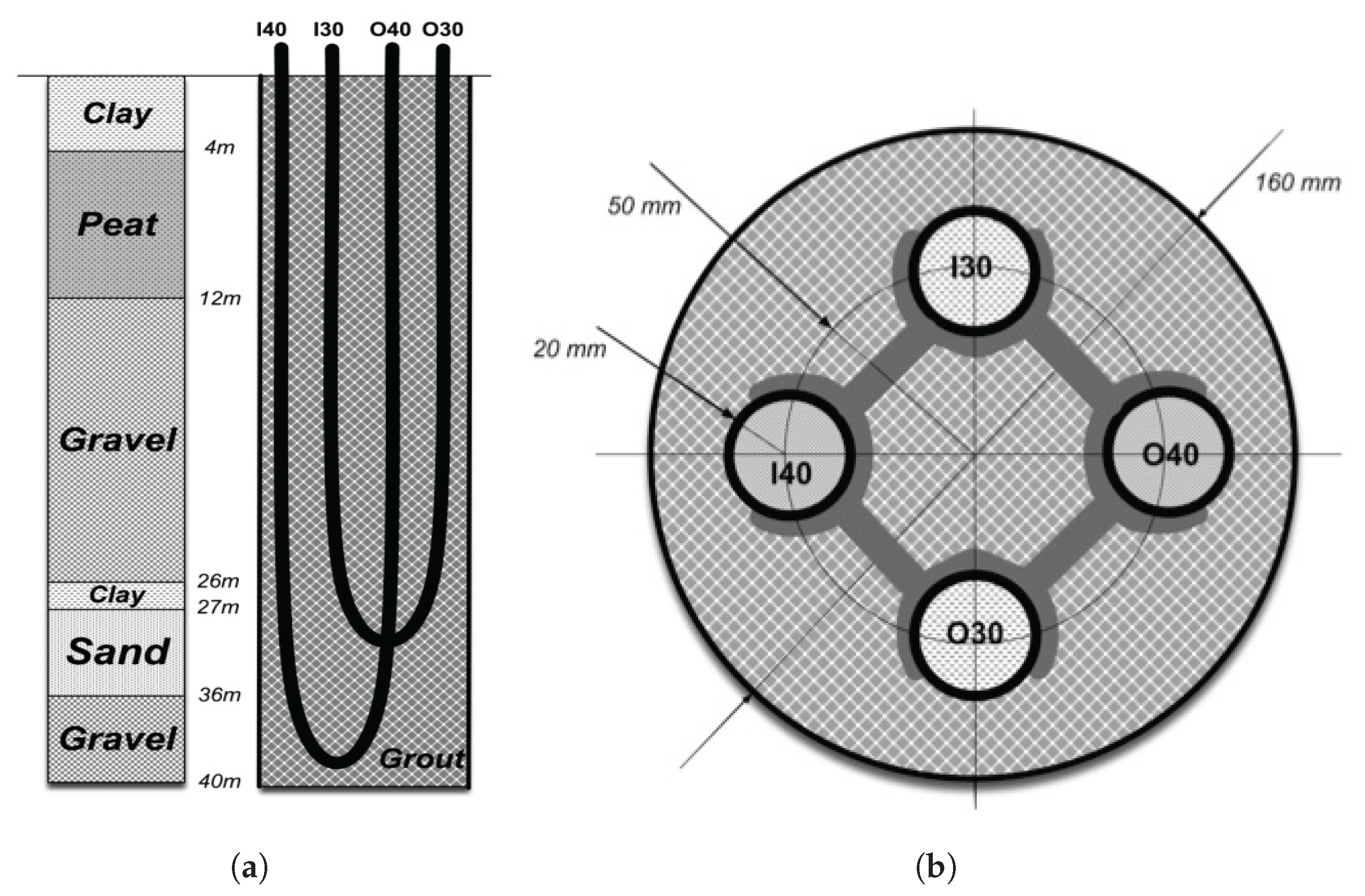
2.1. Description of Borehole Heat Exchanger
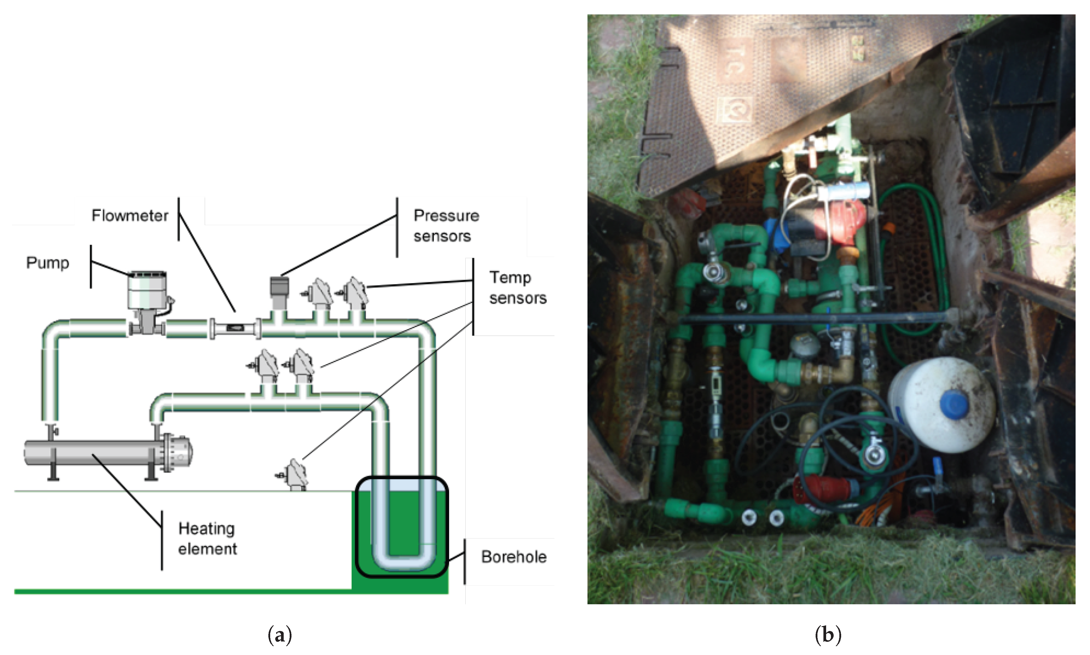
2.1.1. Hydraulic Components and Sensors
2.1.2. System Control and Data Acquisition
- (i)
- the state of the pump (on or off)
- (ii)
- the type of control for the electric immersion heater: PID or a manual
- (iii)
- the reference for internal PID heating control (heat injection rate in kW) or manual setting (fixed rate of use of the electric immersion heater in percentage)
- (iv)
- the sample period for data acquisition in milliseconds
2.1.3. Setting of a TRT Experiment
2.2. Experiments Description
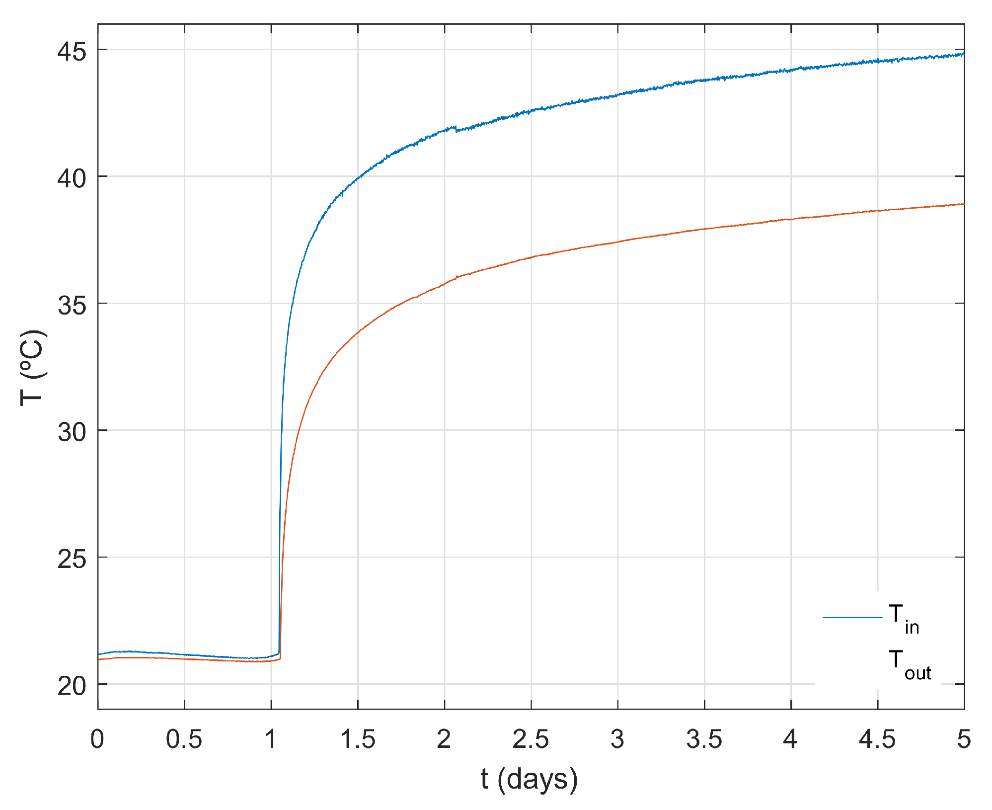
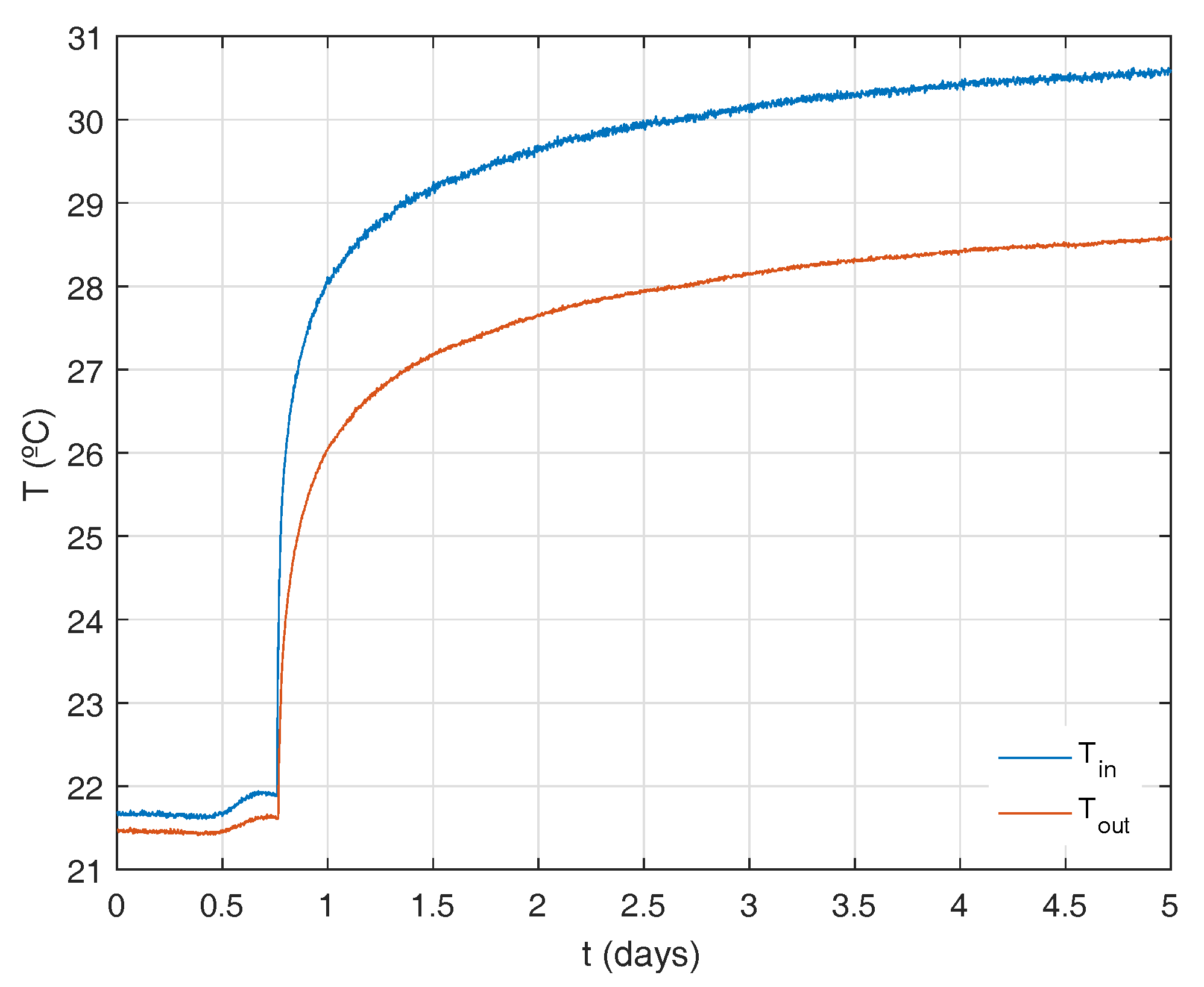
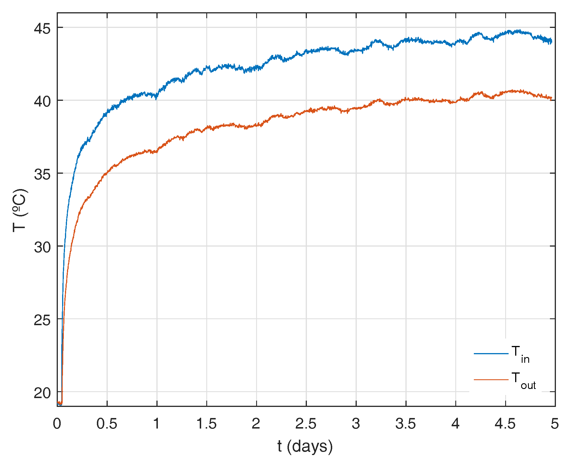
2.2.1. Raw Data Description
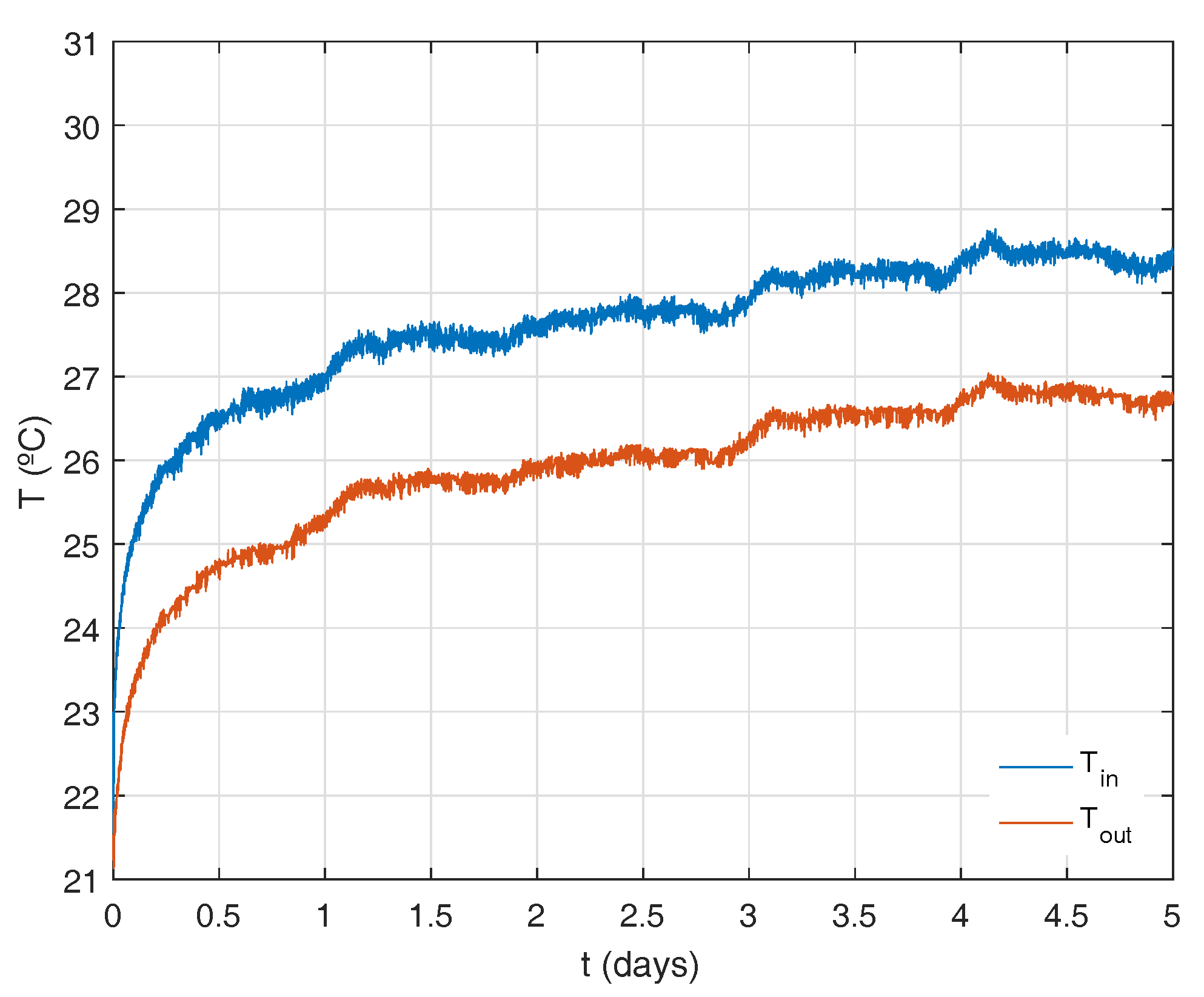
- : temperature at the inlet of the borehole
- : temperature at the outlet of the borehole
- G: water flow
- : ambient temperature
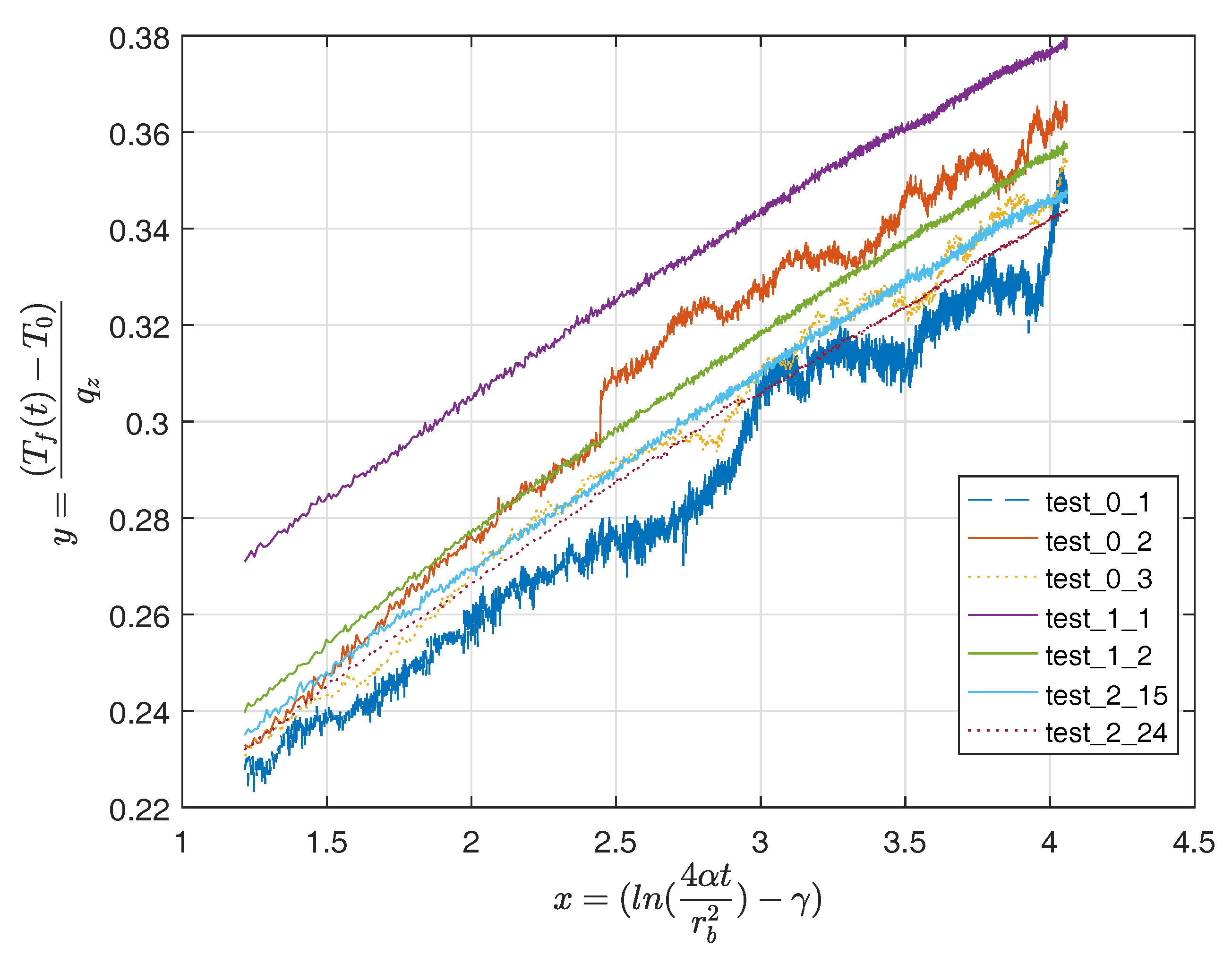
2.3. Data Processing
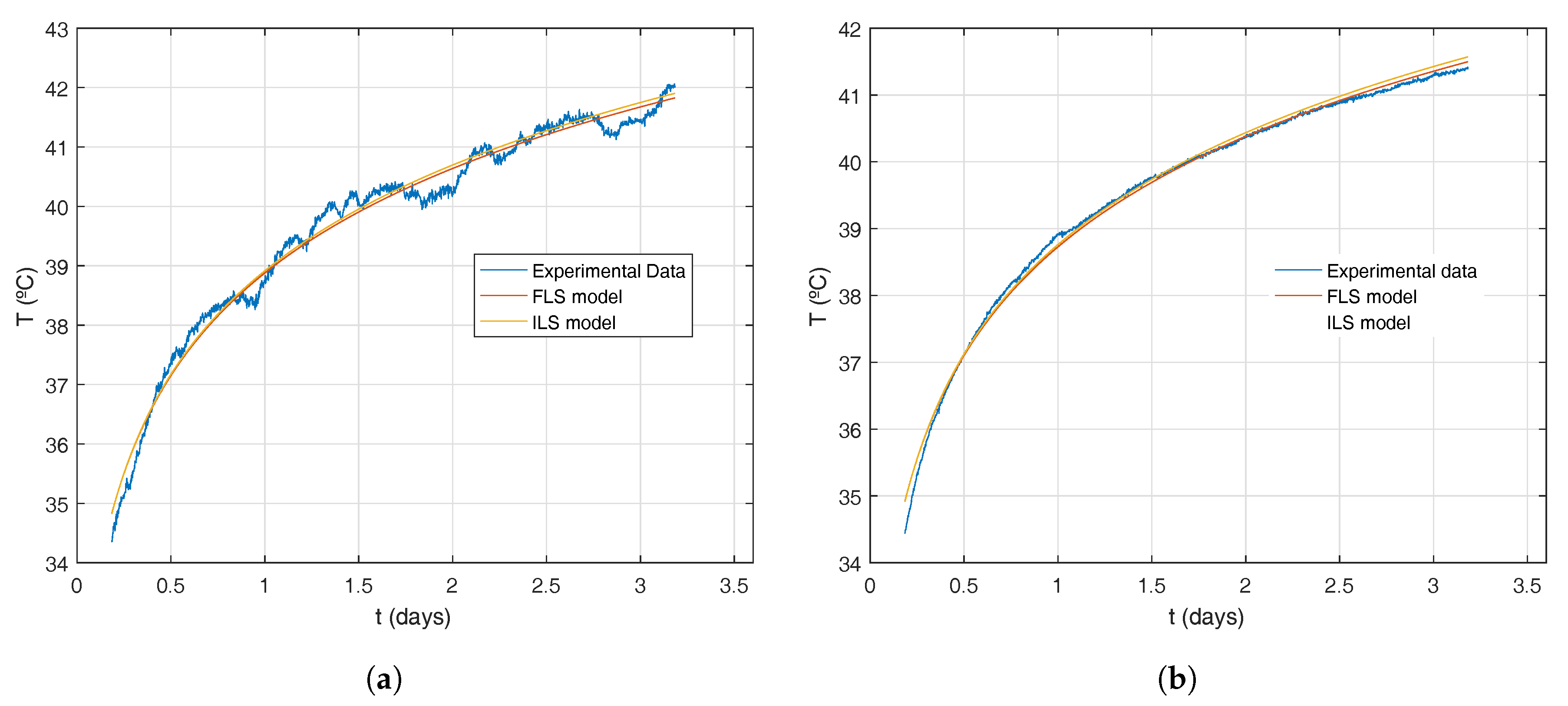
2.4. Application of Different Analytic Models to TRT Data
2.4.1. Infinite Line Source Theory
2.4.2. Least Square Approach with FLS and ILS
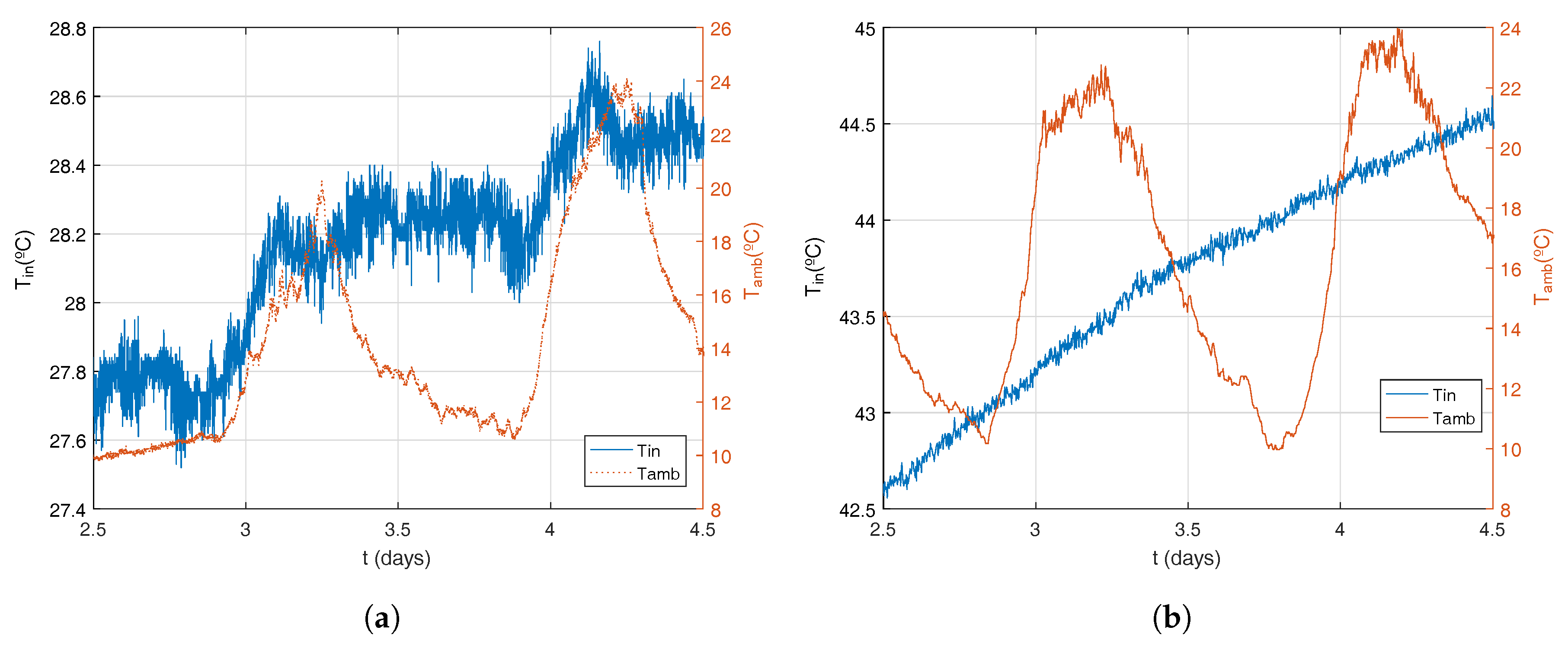
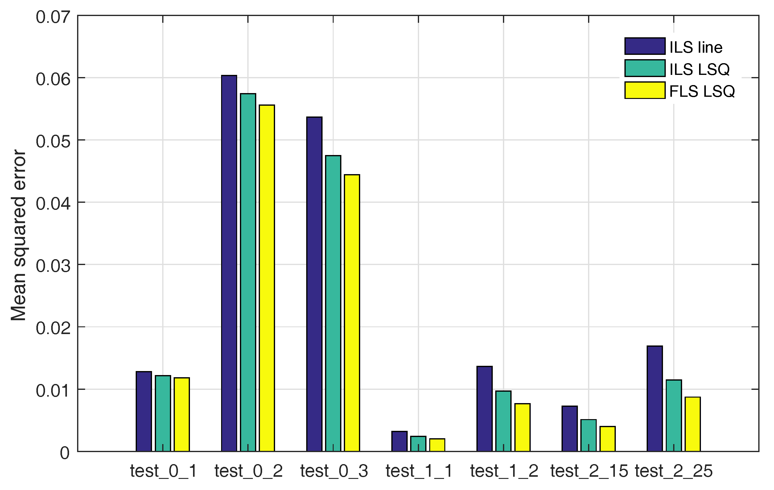
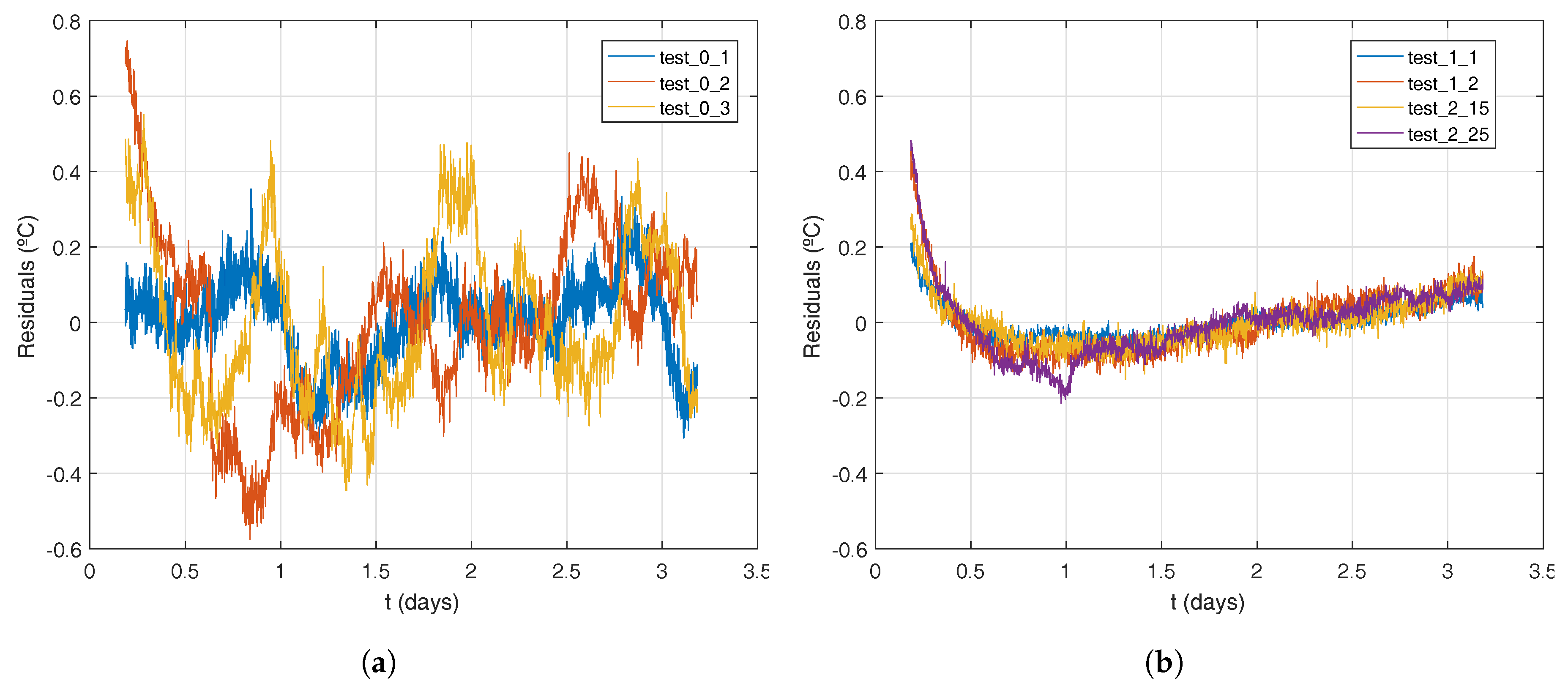
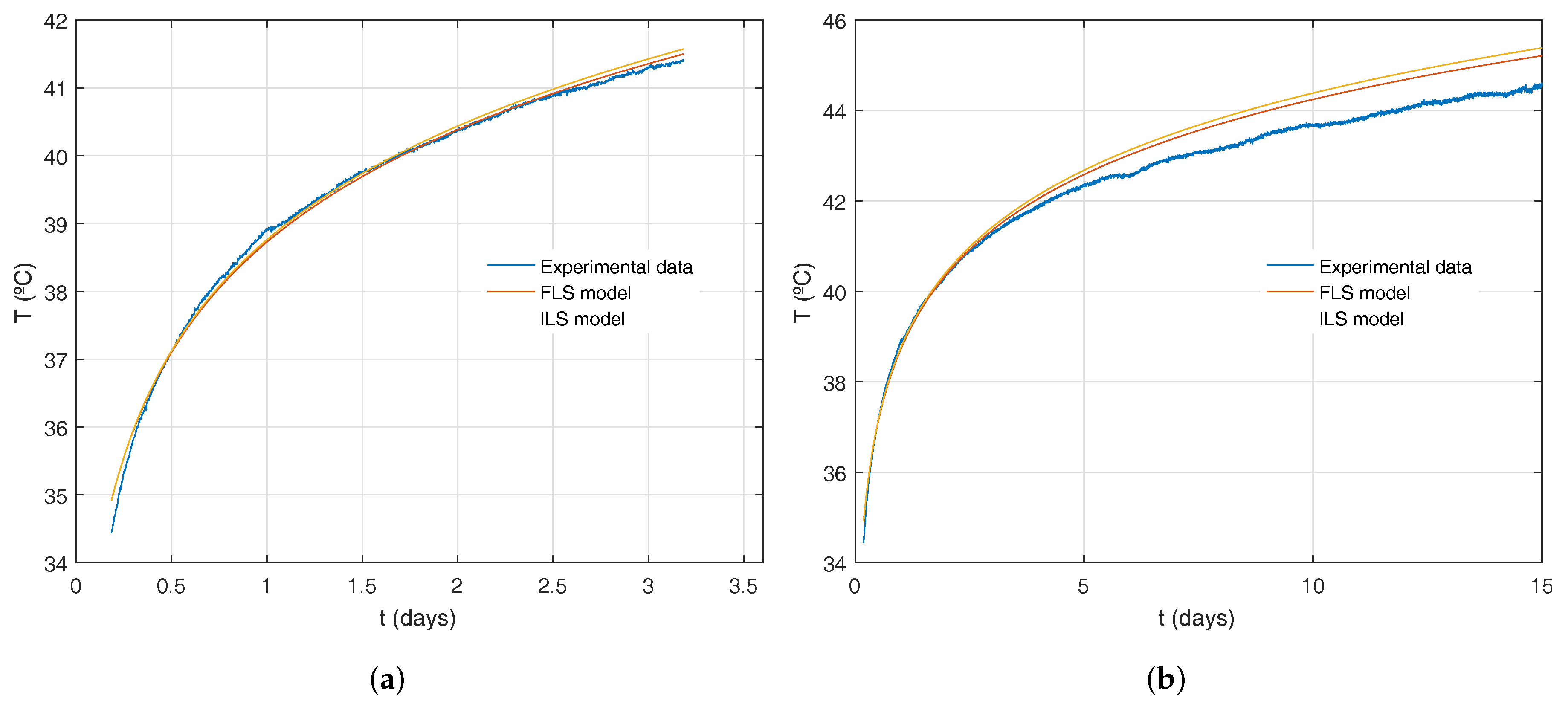
2.5. Model Adequacy and Long Term Effects
3. Conclusions
Acknowledgments
Author Contributions
Conflicts of Interest
Abbreviations
| Abbreviations | |
| UPV | Universitat Politècnica de València |
| HVAC | Heating, ventilation and air conditioning |
| TRT | Thermal Response Test |
| BHE | Borehole Heat Exchanger |
| PID | Proportional, Integral and Derivative |
| PWM | Pulse Width Modulation |
| ILS | Infinite Line Source Model |
| FLS | Finite Line Source Model |
| LSQ | Lest squares fitting algorithm |
| MSE | Mean Squared Error |
| Cheap-GSHPs | Cheap and Efficient Application of reliable Ground Source Heat Exchangers and Pumps |
| GEOCOND | Advanced materials and processes to improve performance and cost-efficiency of Shallow Geothermal systems and Underground Thermal Storage |
| Nomenclature | |
| H | BHE depth (m) |
| temperature observation point distance to the line source (m) | |
| BHE radius (m) | |
| Ambient temperature (C) | |
| Inlet temperature at te BHE (C) | |
| Outlet temperature at te BHE (C) | |
| Mean temperature at the BHE (C) calculated by means of the ILS model | |
| Mean temperature at the BHE (C) calculated by means of the FLS model | |
| Undisturbed ground temperature (C) | |
| G | Water flow (m s) |
| Injected heat flow per unit length (W m) | |
| Water volumetric heat capacity (J m k) | |
| Ground thermal diffusivity (m s) | |
| Ground thermal conductivity (W K m) | |
| Borehole thermal resistance (K m W) | |
| Euler’s constant | |
| ratio between and H | |
| mean of squared residuals |
References
- Gehlin, S. Thermal Response Test—Method Development and Evaluation. Ph.D. Thesis, Department of Environmental Engineering, Luleå University of Technology, Luleå, Sweden, 2002. [Google Scholar]
- Sanner, B.; Hellström, G.; Spitler, J.D.; Gehlin, S. More than 15 years of mobile Thermal Response Test—A summary of experiences and prospects. In Proceedings of the European Geothermal Congress (EGC 2013), Pisa, Italy, 3–7 June 2013. [Google Scholar]
- Witte, H.J.L.; Van Gelder, G.J.; Spitier, J.D. In situ measurement of ground thermal conductivity: A Dutch perspective. Ashrae Trans. 2002, 108, 263–272. [Google Scholar]
- Hellström, G. Ground Heat Storage: Thermal Analyses of Duct Storage Systems. Ph.D. Thesis, Lund University, Lund, Sweden, 1991. [Google Scholar]
- Bandos, T.; Montero, A.; Fernández de Córdoba, P.; Urchueguía, J. Improving parameter estimates obtained from thermal response tests: Effect of ambient air temperature variations. Geothermics 2011, 40, 136–143. [Google Scholar] [CrossRef]
- Bandos, T.V.; Montero, A.; Fernández, E.; Santander, J.L.G.; Isidro, J.M.; Pérez, J.; Córdoba, P.; Urchueguía, J.F. Finite line-source model for borehole heat exchangers: Effect of vertical temperature variations. Geothermics 2009, 38, 263–270. [Google Scholar] [CrossRef]
- De Carli, M.; Tonon, M.; Zarrella, A.; Zecchin, R. A computational capacity resistance model (CaRM) for vertical ground-coupled heat exchangers. Renew. Energy 2010, 35, 1537–1550. [Google Scholar] [CrossRef]
- Lamarche, L.; Beauchamp, B. New solutions for the short-time analysis of geothermal vertical boreholes. Int. J. Heat Mass Transf. 2007, 50, 1408–1419. [Google Scholar] [CrossRef]
- Molina-Giraldo, N.; Blum, P.; Zhu, K.; Bayer, P.; Fang, Z. A moving finite line source model to simulate borehole heat exchangers with groundwater advection. Int. J. Thermal Sci. 2011, 50, 2506–2513. [Google Scholar] [CrossRef]
- Spitler, J.D.; Gehlin, S.E. Thermal response testing for ground source heat pump systems—An historical review. Renew. Sustain. Energy Rev. 2015, 50, 1125–1137. [Google Scholar] [CrossRef]
- Sliwa, T.; Knez, D.; Gonet, A.; Sapinska-Sliwa, A.; Szlapa, B. Research and Teaching Capacities of the Geoenergetics Laboratory at Drilling , Oil and Gas Faculty AGH University of Science and Technology in Kraków (Poland). In Proceedings of the World Geothermal Congress, Melbourne, Australia, 19–25 April 2015. [Google Scholar]
- Montero, A.; Urchueguía, J.F.; Martos, J.; Badenes, B.; Picard, M.A. Ground temperature profile while thermal response testing. In Proceedings of the European Geothermal Congress (EGC 2013), Pisa, Italy, 3–7 June 2013; pp. 1–6. [Google Scholar]
- Eskilson, P. Thermal Analysis of Heat Extraction Boreholes. Ph.D. Thesis, Lund University, Lund, Sweden, 1987. [Google Scholar]
- Badenes, B.; Mateo Pla, M.A.; Magraner, T.; Lemus, L.; Urchueguía, J.F. Experimental facility to perform Thermal Response Tests and study the thermal behaviour of the ground. In Proceedings of the European Geothermal Congress (EGC 2016), Strasbourg, France, 19–14 September 2016; pp. 19–24. [Google Scholar]
- Grundfos Web Page. Available online: https://www.grundfos.com (accessed on 31 July 2017).
- IFM TA3130. Available online: https://www.ifm.com/gb/en/product/TA3130 (accessed on 31 July 2017).
- OSAKA web page. Available online: http://osakasolutions.com (accessed on 1 September 2017).
- IFM SM8000. Available online: https://www.ifm.com/gb/en/product/SM8000 (accessed on 31 July 2017).
- Siemens AG Simatic S7-1200. Available online: http://www.siemens.com/s7-1200 (accessed on 31 July 2017).
- Tinti, F.; Bruno, R.; Focaccia, S. Thermal response test for shallow geothermal applications: A probabilistic analysis approach. Geotherm. Energy 2015, 3, 6. [Google Scholar] [CrossRef]
- Luo, J.; Rohn, J.; Xiang, W.; Bertermann, D.; Blum, P. A review of ground investigations for ground source heat pump (GSHP) systems. Energy Build. 2016, 117, 160–175. [Google Scholar] [CrossRef]
- Austin, W. Development of an In-Situ System for Measuring Ground Thermal Properties. Master’s Thesis, Oklahoma State University, Stillwater, OK, USA, 1998. [Google Scholar]
- Verdoya, M.; Chiozzi, P. Influence of groundwater flow on the estimation of subsurface thermal parameters. Int. J. Earth Sci. 2016, 1–8. [Google Scholar] [CrossRef]
- Badenes, B.; de Santiago, C.; Nope, F.; Magraner, T.; Urchueguía, J.F.; de Groot, M.; de Santayana, F.P.; Arcos, J.L.; Martín, F. Thermal characterization of a geothermal precast pile in Valencia (Spain). In Proceedings of the European Geothermal Congress (EGC 2016), Strasbourg, France, 19–14 September 2016. [Google Scholar]


| Sensor Name | Units | Description | Specification |
|---|---|---|---|
| C | Temperature at borehole inlet | IFM TA3130 [16] | |
| PT100 Class A | |||
| C | Temperature at borehole outlet | Range: 0–140 C | |
| Output: 4–20 mA | |||
| C | Ambient temperature | Res < 0.02 C | |
| Pressure | Pa | System pressure | OSAKA PP10 [17] |
| Range: 0–1000 kPa | |||
| Output: 4–20 mA | |||
| Linearity: 0.3% | |||
| Stability: 0.2% | |||
| Flow | m h | Water Flow | IFM SM8000 [18] |
| Range: 0.01–6.00 m h | |||
| Output: 4–20 mA | |||
| Res < 0.005 m h |
| Experiment | Start Date | Duration | Control | Heat Injection Rate (W) | ||
|---|---|---|---|---|---|---|
| (yyyy-mm-dd) | (Days) | Reference | Mean | Standard Deviation | ||
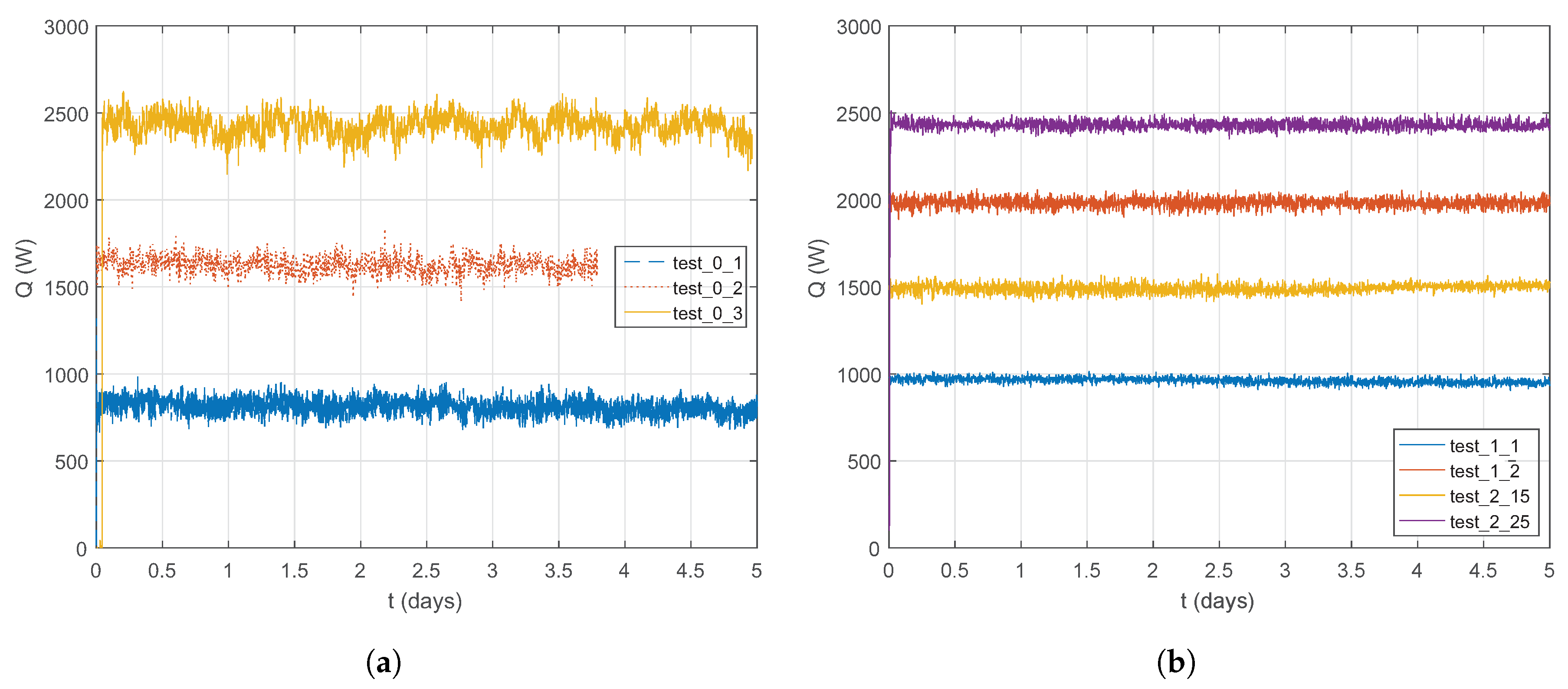
| test_0_1 | 2011-09-25 | 10 | None | 1000 | 795 | 39 |
| test_0_2 | 2012-02-10 | 3.5 | None | 2000 | 1626 | 51 |
| test_0_3 | 2012-03-10 | 7 | None | 3000 | 2405 | 66 |
| test_1_1 | 2015-10-21 | 12 | PID | 1000 | 954 | 17 |
| test_1_2 | 2016-03-07 | 11 | PID | 2000 | 1982 | 26 |
| test_2_15 | 2017-03-07 | 9 | PID | 1500 | 1497 | 24 |
| test_2_25 | 2017-04-10 | 31 | PID | 2500 | 2428 | 22 |
| Experiment | a | b (=R) | (= | |||
|---|---|---|---|---|---|---|
| test_0_1 | 0.0394 | 0.0003 | 2.02 | 0.02 | 0.179 | 0.0012 |
| test_0_2 | 0.0422 | 0.0008 | 1.89 | 0.04 | 0.195 | 0.0027 |
| test_0_3 | 0.0403 | 0.0005 | 1.97 | 0.02 | 0.187 | 0.0016 |
| test_1_1 | 0.0365 | 0.0002 | 2.18 | 0.01 | 0.233 | 0.0007 |
| test_1_2 | 0.0397 | 0.0002 | 2.01 | 0.01 | 0.198 | 0.0007 |
| test_2_15 | 0.0387 | 0.0002 | 2.06 | 0.01 | 0.193 | 0.0007 |
| test_2_25 | 0.0379 | 0.0002 | 2.10 | 0.01 | 0.191 | 0.0007 |
| Experiment | ILS Line | ILS | FLS | |||
|---|---|---|---|---|---|---|
| test_0_1 | 2.02 | 0.179 | 1.93 | 0.173 | 1.95 | 0.173 |
| test_0_2 | 1.89 | 0.195 | 1.80 | 0.188 | 1.82 | 0.189 |
| test_0_3 | 1.97 | 0.187 | 1.88 | 0.180 | 1.91 | 0.181 |
| test_1_1 | 2.18 | 0.233 | 2.08 | 0.227 | 2.11 | 0.227 |
| test_1_2 | 2.01 | 0.198 | 1.91 | 0.191 | 1.94 | 0.192 |
| test_2_15 | 2.06 | 0.193 | 1.96 | 0.186 | 1.99 | 0.187 |
| test_2_25 | 2.10 | 0.191 | 2.00 | 0.185 | 2.03 | 0.186 |
© 2017 by the authors. Licensee MDPI, Basel, Switzerland. This article is an open access article distributed under the terms and conditions of the Creative Commons Attribution (CC BY) license (http://creativecommons.org/licenses/by/4.0/).
Share and Cite
Badenes, B.; Mateo Pla, M.Á.; Lemus-Zúñiga, L.G.; Sáiz Mauleón, B.; Urchueguía, J.F. On the Influence of Operational and Control Parameters in Thermal Response Testing of Borehole Heat Exchangers. Energies 2017, 10, 1328. https://doi.org/10.3390/en10091328
Badenes B, Mateo Pla MÁ, Lemus-Zúñiga LG, Sáiz Mauleón B, Urchueguía JF. On the Influence of Operational and Control Parameters in Thermal Response Testing of Borehole Heat Exchangers. Energies. 2017; 10(9):1328. https://doi.org/10.3390/en10091328
Chicago/Turabian StyleBadenes, Borja, Miguel Ángel Mateo Pla, Lenin G. Lemus-Zúñiga, Begoña Sáiz Mauleón, and Javier F. Urchueguía. 2017. "On the Influence of Operational and Control Parameters in Thermal Response Testing of Borehole Heat Exchangers" Energies 10, no. 9: 1328. https://doi.org/10.3390/en10091328