1. Introduction
Synthetic power grids are test cases that are not based on any real power system. The motivation for building such cases it that real grids are subject to data confidentiality restrictions, and usually real power system cases cannot be shared publicly. Existing public cases, such as the IEEE test cases [
1], are relatively modest in size and complexity, and thus do not fully meet the needs of the power systems research community today. A few other cases are available, including the large model introduced by [
2], which is only suitable for dc power flow and approximates the real European grid. New synthetic test cases are being developed, and have many benefits for power engineering researchers to spur innovation, encourage reproducibility of results, and enhance peer review, all while respecting the secure nature of actual grid model data.
The network topology of power systems has been the subject of significant study, traceable at least to study [
3], where a small-world model was proposed that showed common properties in graph structure with other real world networks. References [
4,
5,
6,
7] and others expanded on this topic with particular reference to transmission grid networks, finding applications of the graph theory analysis to system operation, security, and stability. It is certain that power grids, in light of their geographic constraints and design for secure operation, have particular network structure characteristics that are consistently observed across systems. Among the metrics studied, a short average path length, high degree of clustering, exponential degree distribution, and average nodal degree around 2.3–2.8 are documented as typical of power grid graphs.
These topological metrics have been applied in studies [
8,
9,
10,
11,
12] to synthetic power grids, both as pieces of a network generation algorithm and as validation criteria for networks considered. A pure small-world model or other random graph is not sufficient [
4]. After all, power grids are certainly not random; rather, they are carefully planned. The degree distribution is approximately exponential, but with the exception that nodes of degree one (radial) are much less prevalent. The approach of the authors of [
8] is to modify the small-world model, producing network topologies. The approach in study [
10] use a clustering-connect method to reproduce the local connectivity structures. More recently, studies [
11] and [
12] consider the importance of geographic location in network structure, since these constraints dominate the actual grid’s planning process.
The driving design standards for synthetic power grids are the actual grid models themselves, since the objective is for synthetic grids to be as realistic as possible. A methodology for generating full transmission system models, including everything needed for full ac power flow solutions, was documented in study [
13] and further developed in study [
14]. The approach is substation-oriented with a focus on geographic constraints. To reduce the edge search space, it uses the Delaunay triangulation, which is a graph from computational geometry constructed to identify a set of points’ nearest neighbors. The approach also considers nominal voltage levels, to implement the local clustering and long-distance short paths. Systems with size 150 buses and 2000 buses are described and released.
The process begins with public geographic information on generation and population in an area, from which synthetic substations are placed geographically. Then buses are added to these substations, connected by transformers and a network of transmission lines, using an iterative process that considers multiple factors. Base case models can also be extended with additional complexities for a variety of types of studies [
15,
16,
17,
18]. To validate these models, the authors of [
13,
14] give statistics on the typical topological criteria from earlier work as well as new observations about the Delaunay triangulation and the general proportions of load and generation. However, the set of actual systems studied for reference, the acceptable metric qualifications, and the coverage of parameters through validation is preliminary.
Validating full power system models, that is, determining how accurately their features match what is found in the actual grid, is key to ensuring the quality of new synthetic power grids for their use in research and development. This paper presents a systematic approach to validation, and contributes many new validation metrics and their defined criteria to match. These metrics are designed to help quantify the realism of a synthetic grid. Because of the variety in engineering design and modeling practices, actual grids are quite diverse; the interesting challenge in this work is to capture the distribution of network characteristics, in a way that synthetic grids can be adequately evaluated. In addition, the size of a network can affect its statistical properties, since large networks have averaging effects. Each of these issues is addressed in this paper by studying a high-quality, diverse, large set of North American power system models. The initial suite of validation metrics defined here contributes a benchmark for developed cases.
2. Proposed Validation Methodology
Every aspect of the proposed synthetic grid validation is anchored in a thorough analysis of high-quality real power grid models. The actual power system data for which statistics are given in this paper comes from observations of the major North American power grid interconnections, as obtained from the Federal Energy Regulatory Commission (FERC) form No. 715 dataset [
19], as well as twelve subset cases created by extracting areas along geographic and utility lines from the full interconnects. From these, statistics are gathered on cases ranging from 400 to 5000 buses, in addition to the 70,000 and 16,000 buses in full eastern (EI) and western (WECC) interconnect cases, respectively. These studied cases are listed in
Table 1, with the number of buses shown.
The framework of this validation process is broad in application, since collecting statistics on system properties and identifying benchmarks is appropriate for many aspects of the power system which may be synthesized. The focus of the metrics selected for this paper, however, is in two categories: the metrics of system proportions and those of system network. Together, these categories cover much of what is needed for a base case power flow solution. The idea in picking metrics is to obtain wide coverage of parameters. Except transmission lines, everything in power system models are contained in substations, so these aggregations are the orientation of the questions answered by selected metrics—How many substations are there? What voltage levels do they contain? How much load and generation do they have? Then more detailed metrics are studied that set the power flow parameters of loads and generators. Covering the branch topology is the objective of the second set of metrics. Here, substation transformers are studied in their impedance and limit parameters. The same is studied for transmission lines, followed by topological observations, which likewise are focused on substations and voltage levels. At each stage, coupling is considered among metrics; clearly nominal voltage level will significantly impact transmission line impedance, for example.
For each metric selected, a quantitative threshold standard is decided, with the expectation that no realistic power system will violate that standard, unless there is an exception that has a justification in engineering design choice. In other words, this validation is a screening process that looks at almost all parts of the grid model and picks out any unusual data for further scrutiny. Exceptions of this type are part of the diversity of engineering practices among many grids. The case size must also be considered when looking at exceptions, as large cases are bound to have a few outliers, but will have much more consistent trends than smaller cases, which are more sensitive to the peculiarities of location.
3. Metrics of System Proportions: Substations, Load, and Generation
Number of buses per substation. Substation aggregation of buses indicates how buses are related to a specific geographic location. While substation grouping and geographic location are not strictly necessary for power flow solutions, they are integral to an understanding of grid topology, since geography is a major driving factor in system design.
The EI averages 2.3 buses at each substation, and the WECC averages 2.5. The subset cases considered vary from 1.7 buses per substation to 4.5. The number of buses represented in each substation can be affected by modeling decisions about how much detail is represented, including generator step-up transformers and sub-transmission network equivalents.
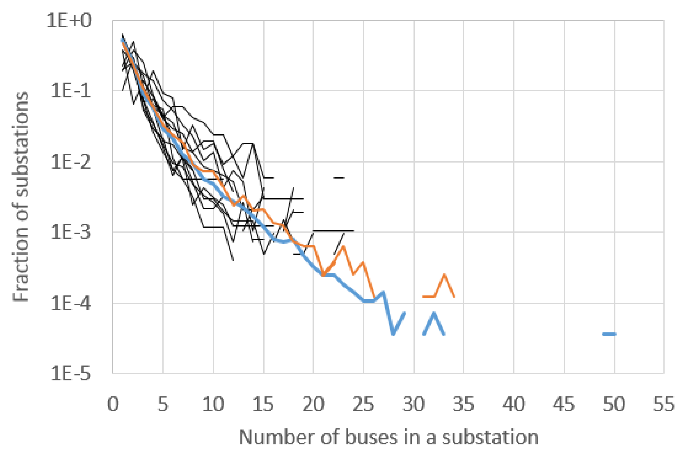
Figure 1 shows the distribution of substation size. There are many substations with 1–3 buses, much fewer with 4–10 buses, and fewer still with 10–25. The larger the case is, the longer the tail of this distribution, as
Figure 1 shows. For cases on the order of 100 buses, the tail could end at about the 1% threshold, which would make a largest substation of about 8 buses acceptable. The EI and WECC cases (orange and blue in
Figure 1) have on the order of 10000 buses; their tail extends to the 1 × 10
−4 threshold at about 27 buses.
Substation voltage levels. The synthetic networks will focus on transmission nominal voltage levels of 69+ kV.
Table 1 shows the percentages of such substations with buses in the 69–200 kV range and the 200+ kV range, for each of the fourteen cases. The majority cluster of areas in
Table 1 indicates synthetic networks should have a 69–200 kV bus at 85–100% of substations, and 7–25% of transmission substations should have a bus in the range 201+ kV. The two exceptions to this rule, areas 8 and 10, use 230 kV as a system-wide voltage, while the rest of the areas use a voltage below 200 kV for a system-wide network. Synthetic networks could be designed in this way, in which case substations with 230 kV would fall in the lower category rather than the upper one.
Percentage of substations containing load. Categorizing buses or substations as load, generating, or neither plays an important role in synthesis methods and relates to the core energy delivery purpose of power systems. Except for two cases, areas 5 and 9, all of those studied show 75–90% of substations containing load, as shown in
Table 1. Load, of course, is an aggregation of sub-transmission, distribution, and customer-level circuits, which for these exceptions appears to be grouped at a higher level than for typical grid cases.
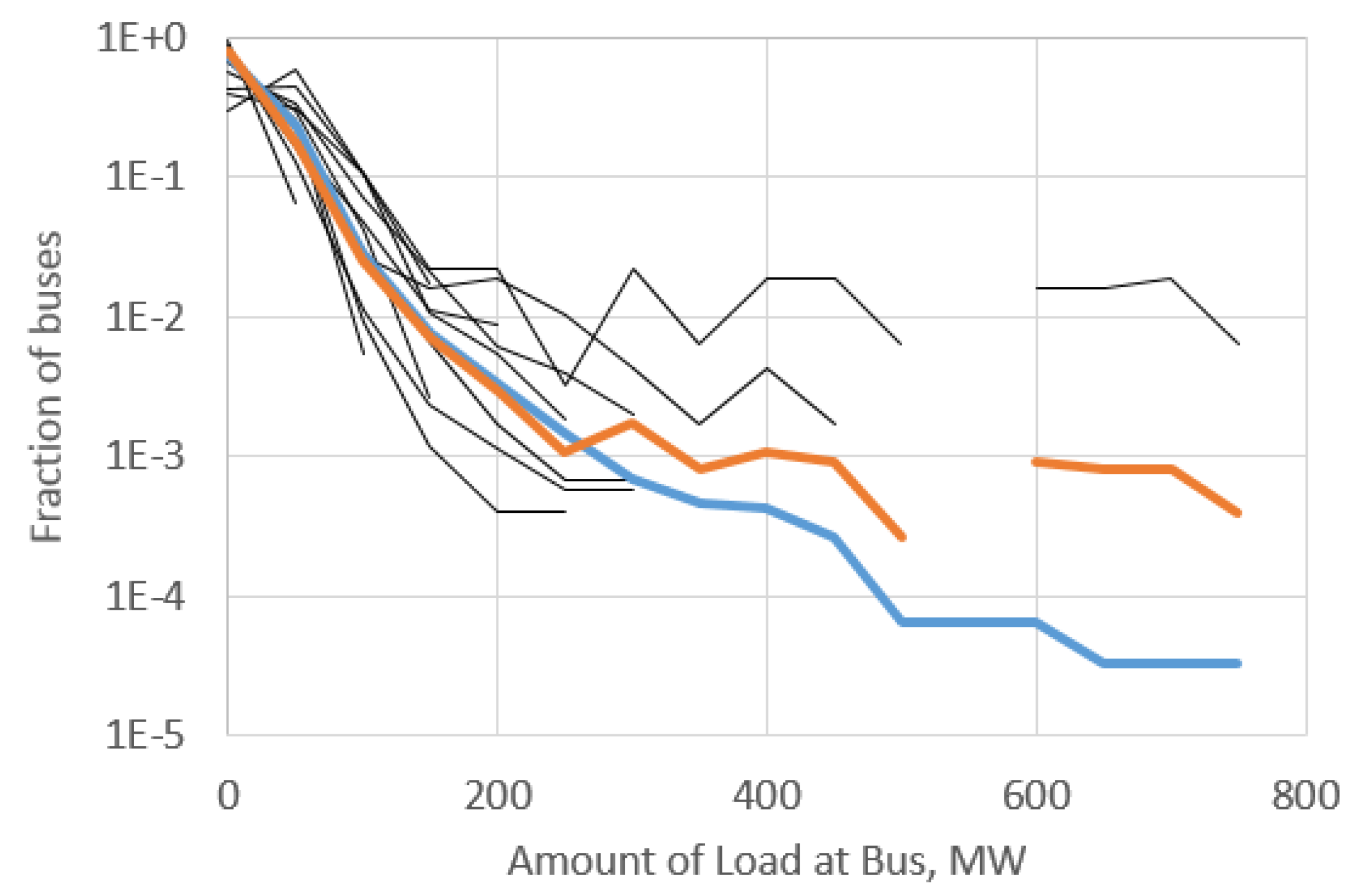
Load at each bus. The selected cases vary from about 6–18 MW of load per bus on average. This excludes a couple of cases, which, because of their large net import or export of power, are outliers. Synthetic networks are often designed as self-contained systems. This average metric is important because it indicates the relationship between the size of a network in buses and the amount of peak load it serves.
Figure 2 shows the distribution of bus loads, for buses which have at least one load. The distribution varies widely, depending on the aggregation decisions used to model the loads at each bus. However, all cases show a large number of smaller loads, with a smaller percentage of larger ones. This distribution should be met in synthetic cases.
Ratio of total generation capacity to total load. The EI and WECC and their sub-regions generally have 20–60% more generation capacity than the peak load, as shown in the rightmost column of
Table 1. There are two exceptions, one which imports lots of power and has 12% less generation capacity than total load, and one which has 104% more capacity as it exports a lot of power. The other cases fall within the realistic range of 20–60% capacity surplus. For any self-contained system, this metric should be almost inviolable.
Percent of substations containing generation. In the EI, 11% of substations contain generation, and in the WECC, the proportion is 17%. The values are shown in the sixth column of
Table 1. Several of these cases tend to be outliers, since this metric is also related to the sort of generators that are used in a particular area and how many small generators are modeled. The defined metrics is that synthetic cases should contain generation in 5–25% of substations, which centers around the aggregate statistics from the full interconnects and includes most of the actual cases studied.
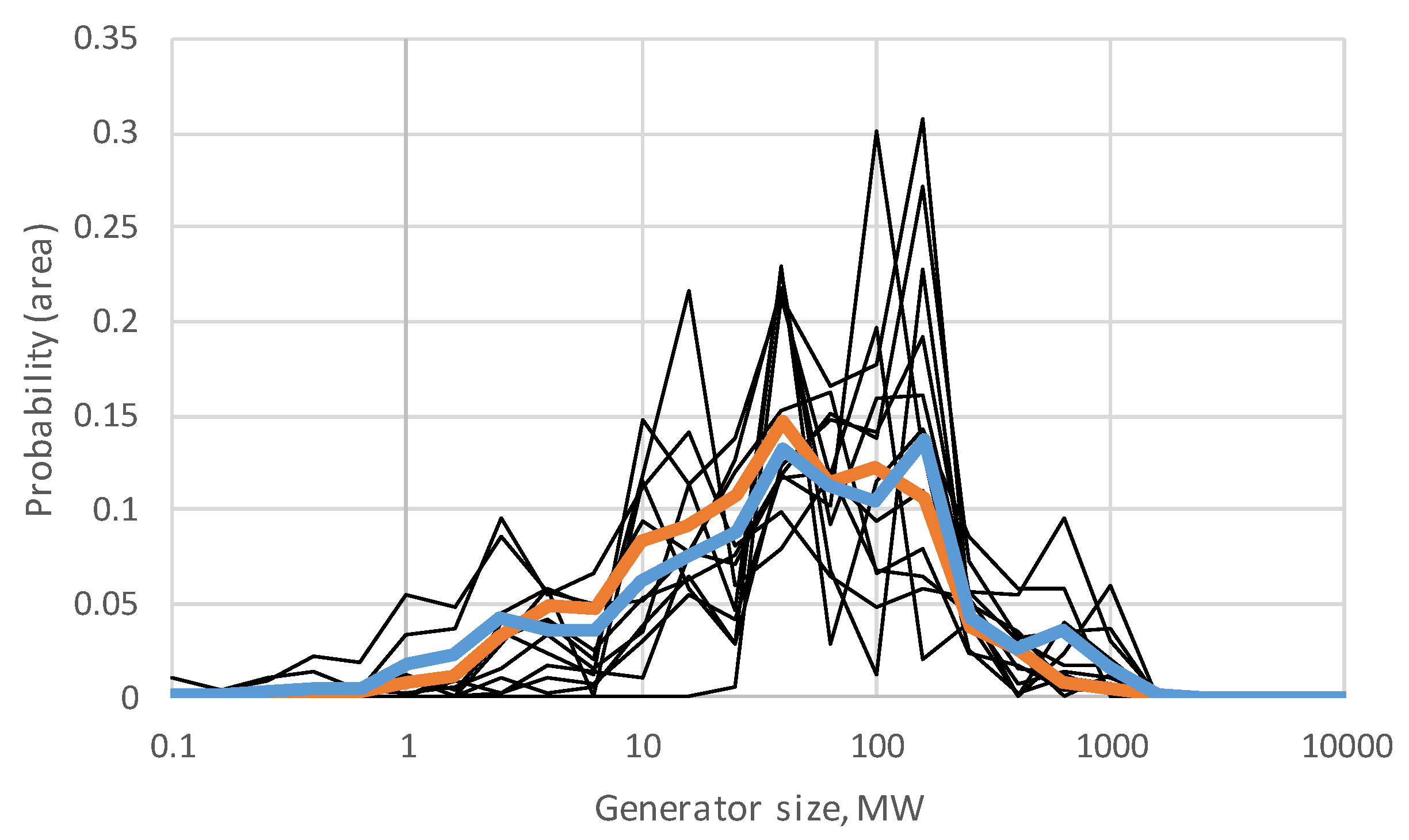
Capacities of generators. The selected cases consistently contain a wide variety of generator MW capacities, and it is important for synthetic cases to contain not only the correct total and average generation, but the spectrum of generator sizes real cases contain.
Figure 3 shows these cases, with the range of 25 MW to 200 MW being the most common range for all cases, and most cases containing a few generators larger than 200 MW. Below 25 MW, the modeling varies. Some cases include a sizeable set of small generators, while at least a few areas largely ignore or aggregate them.
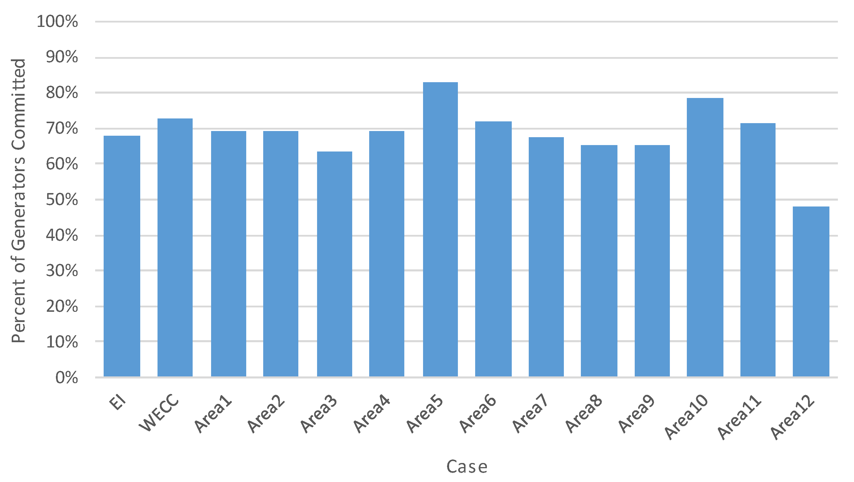
Percent of generators committed. The percent of generating units which are committed, that is, connected to the grid and generating power positive active power, is an important metric of the reserves and economics of the generation fleet. As shown in
Figure 4, this value is 60–80% for most of the real cases considered.
Generator dispatch percentage. Most committed generators in peak planning cases are operated close to their maximum MW capacity. This is especially true in certain areas of the EI. Recognizing the wide variation of this parameter, as illustrated in
Figure 5, the defined criterion is that at least 50% of generators should be dispatched above 80%. The EI and WECC are shown to have diverging distributions, nevertheless, they share the characteristics that the majority of generators are operated close to their MW limit. Parameters closely tied to operational considerations such as this one will change over time and show larger variance, but the focus is on the planning case values and capturing the salient characteristics.
Generator reactive power limits. Generators’ ratio between maximum reactive power limit and maximum active power limit, MaxQ/MaxP, shows the relationship between the size of a generator and how much voltage support it can give. This parameter also has a wide range of variety, since in actuality these are approximations for the capability curves, since reactive power limits are not the same at each active power operating point. As a basic qualification that seems to meet the data in real cases, for at least 70% of generators, that ratio of maximum reactive power to maximum active power should be between 0.40 and 0.55.
4. Metrics of System Network: Transformers and Transmission Lines
This set of validation metrics focus on the parameters of system branches and their topology. For transformers, the topology is straightforward: they connect different voltage levels within substations. For lines, the Delaunay triangulation metrics are repeated as excellent proxies for many of the network characteristics that previous work has studied. The network parameters are given, with due attention to the coupling that resistance, reactance, line length, and voltage levels can involve.
Transformer per-unit reactance. Transformer reactance X is evaluated on the transformer power base in MVA,
, which is related to the
value used in the power flow case by the formula:
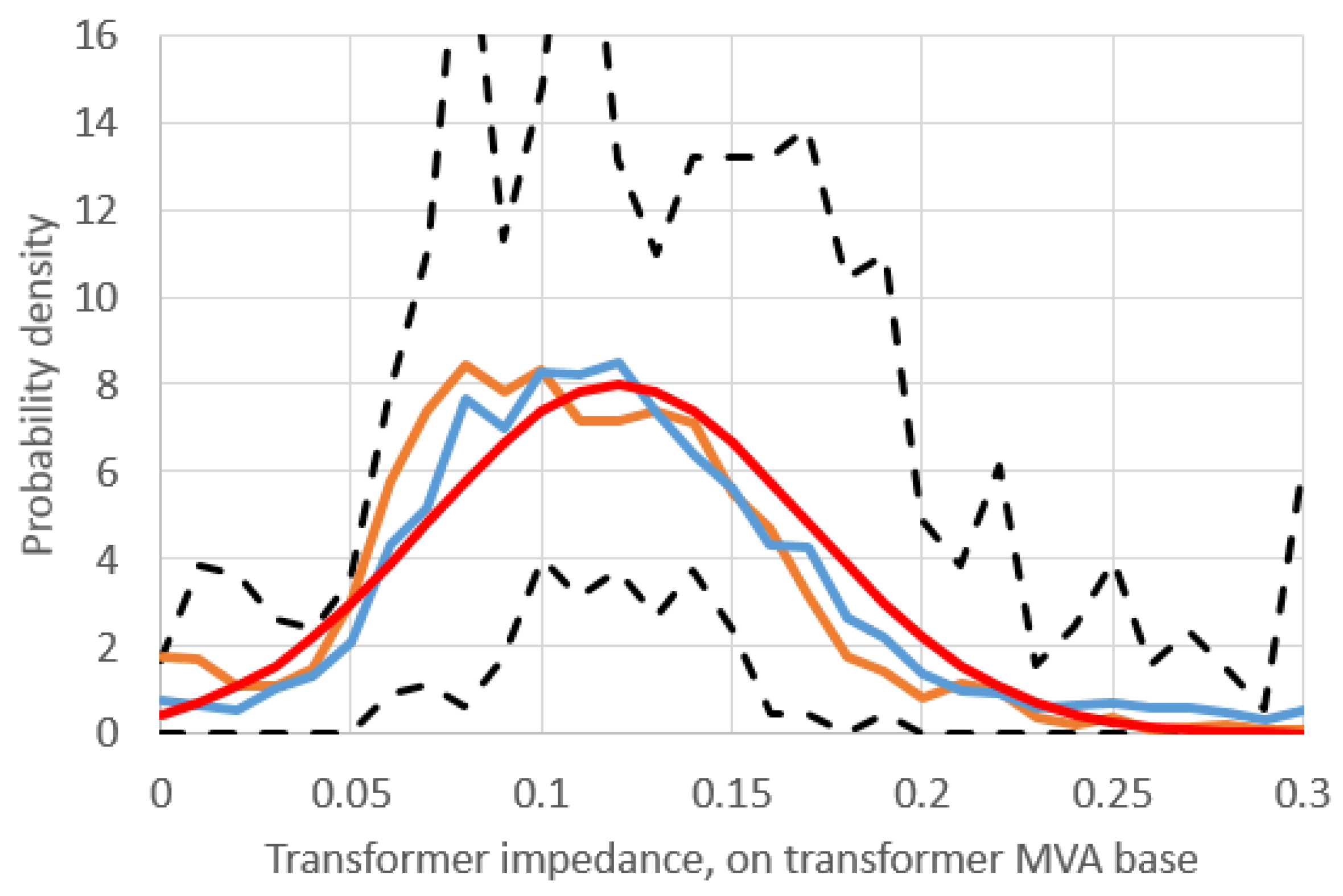
Analysis shows in the transformer reactance parameters a rather consistent distribution, when viewed in per-unit on the transformer base values.
Figure 6 shows the density functions for each case, along with a normal fit. It is typical for at least 80% of transformers to have a reactance value in the range [0.05, 0.2], and the distribution is roughly normal, centered around 0.12, with some variation as shown in the figure.
Transformer MVA limit and X/R ratio. Transformer MVA limit and X/R ratio statistics include outliers for large cases, because R and MVA limits for transformers are not absolutely essential to power flow studies. Sometimes a default small R value is used, so that the X/R ratio appears to be 10000 or more, which is unlikely to be accurate. However, for many transformers the data is reliable.
It is found that the transformer high voltage level is well correlated with both of these characteristics. Thus the analysis is printed in
Table 2 organized by voltage level for both the EI and WECC. The main objective is to see the common range of values for each level of transformer.
The validation criteria for MVA limit and X/R ratio are based on the median value, as well as the 10th and 90th percentile values. Cases should have at least 80% of transformer values within the 10th and 90th percentiles, and at least 40% above and 40% below the median. The less constrained of the EI and WECC values can be used.
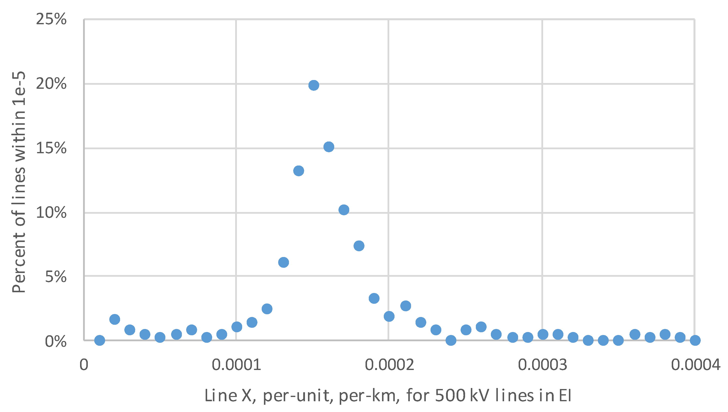
Transmission line reactance. Transmission line parameters are organized by voltage level, since many aspects of transmission line design depend on the voltage level. The per-unit reactance depends heavily on the length of the transmission line, which, while not available exactly, can be approximated from the geographic distance between the two substations it connects. This distance will always be shorter than the actual right-of-way length, but serves as an approximation, especially for longer lines. Transmission line per-km impedances at a certain nominal voltage level typically have a unimodal distribution with heavy tails corresponding to outliers, as shown in
Figure 7. Some of the outliers may be due to smaller transmission lines for which the per-distance metric is less accurate. Similar to the transformer parameters, the transmission line statistics used are the 10th percentile, the 50th percentile (median) and the 90th percentile. This encompasses most transmission lines.
Table 3 shows these percentages. Data on the distribution of transmission line parameters is also significantly impacted by the number of conductors bundled together in a phase, with 2- and 3- conductor bundling reducing the 345 and 500 kV lines.
Transmission line X/R ratio and MVA limit. In the same way, the 10/50/90 percentiles were calculated for transmission line X/R ratio and MVA limit, for major voltage levels, as shown in
Table 4. Reference [
18] has also examined MVA limit for transmission lines. These statistics do not consider transmission lines whose R values or MVA limits are not given. It is noticeable how narrow the 10–90 window is in each statistic, indicating the relatively consistent range in which realistic line parameters fall. The rule-of-thumb for validation, allowing for some variability, is for at least 70% of lines to fall inside the 10–90 window. Synthetic transmission lines are also validated during construction if they are synthesized from actual conductors and tower configurations, as described in [
12] and done for synthesized cases in this paper.
Ratio of transmission lines to substations, at a single nominal voltage level. The next set of metrics relate to the most-studied aspect of power grid synthesis: the transmission line topology. While the complex network literature has approximated the topology analysis with random models such as small-world [
3,
5,
7,
8], others have discussed the limitations of such a model because of its deviations from node distribution and its highly-designed, static topological nature [
4,
9,
12].
It is important to define how the power system is viewed as a graph. Because bus modeling, aggregating circuit nodes, can vary within a substation and be more dependent upon breaker configuration, the focus is on substation topology, where substations are the graph vertices and actual transmission lines connecting different substations are the edges. Since there is a special distinction and connectivity limitation between branches of different nominal voltage levels, most of the transmission line topology statistics are also based on individual networks at a single nominal voltage level. Statistics were created by dividing the studied cases into their line topologies, using substations as the graph vertices at 115 kV, 230 kV, 345 kV, 500 kV, etc.
The first fundamental statistic, ratio of lines to substations, is measured for grids at a certain nominal voltage level, and expresses the expected number of transmission lines present, given the number of substations containing the voltage level. This topological metric encompasses the density and redundancy of the graph, as well as average nodal degree. For actual cases, this was evaluated by looking at subset networks with at least 50 substations at voltage levels of 115 kV and higher, as shown in
Table 5. The result was that all networks fall roughly in the range of 1.1–1.4 for the ratio of transmission lines to substations.
Percent of lines on the minimum spanning tree. The Euclidian minimum spanning tree (MST) is the minimum distance graph which connects all substations at a voltage level. This statistic, along with the following Delaunay triangulation statistics, helps to capture the geographic constraints of transmission line networks. Using the spatial relationships between nodes as key to understanding the topology is central to the approaches of [
9,
11], and [
13]. Reference [
13] shows the fraction of actual lines which come from MST, Delaunay, and Delaunay neighbors in EI and WECC, with the MST percentage around 50%.
Distance of transmission lines along the Delaunay triangulation. The Delaunay triangulation is calculated from a set of coordinates, dividing the plane into triangles, in which no triangle’s circumcircle contains another point [
20]. As shown in [
12], which appears to be the first application of this technique to power grid synthesis, most transmission lines have a very short distance along it, and this is an excellent metric of the geographic constraints of transmission line topologies. This reference shows about 75% of lines are on their Delaunay triangulation, about 20% are second neighbors, and about 5% are third neighbors. The number of lines that are fourth neighbors and higher is consistently below 1%.
There are a variety of topology-related graph theory statistics, including the distribution of nodal degrees, clustering coefficient, and average shortest path length, for which transmission networks have distinguished characteristics that have been explored in previous work [
3,
4,
5,
6,
7,
8,
9,
10,
11,
12,
13]. References [
12,
13] have shown that matching the Delaunay triangulation statistics often encompasses the key graph characteristics observed on actual cases, in addition to respecting the geographic constraints of power grids, since transmission lines in general connect nearby substations.
Ratio of total length of all lines to the length of the minimum spanning tree. This metric compares line length at a nominal voltage level to the minimum length needed to connect all the substations, i.e., the length of the minimum spanning tree. These values are shown in
Table 5. For networks above 100 kV and larger than 50 substations, most have this ratio between 1.4 and 2.6. In addition to the relative consistency in this ratio, the driving intuition is that it measures the relationship between the actual size of a power grid and the theoretical geographic minimum required.
5. Validating Two Example Cases
The above validation metrics were applied when building two new synthetic test cases described by this section. The methodology used for building the cases is fundamentally the same as that presented in [
13], tuned to target the validation tests identified in this paper. These cases are available online [
1]. This section uses these cases as an example to show the validation process and verify the realism of these cases.
The 200-bus case ACTIVSg200 was built on the geographic footprint of fourteen counties in central Illinois, an area with a population of about 1.1 million. First, 160 loads based on census data are placed along with 49 generating units coming from public reports, and these are combined into a set of 111 substations. The case has 230/115 kV grids, with buses assigned to substations and the branch topologies generated using an iterative dc power flow selection process, as described in previous work [
12]. A one-line diagram of this case can be seen in
Figure 8a. Branch ac power flow parameters are defined consistent with the geographic lengths as well as the validation metrics, and four shunt capacitors are added for voltage support. Generator cost curves are added using a method similar to [
15], so that an optimal power flow (OPF) solution can be found for this grid.
The 500-bus case ACTIVSg500 was built on the geographic footprint of 21 counties in western South Carolina, an area with a population of about 2.6 million. There are 208 substations with 206 loads and 90 generating units, and an added 15 switched shunt capacitors. The case has 345/138 kV grids, and its one-line diagram can be seen in
Figure 8b. It also has parameters sufficient for an ac power flow solution and an OPF solution.
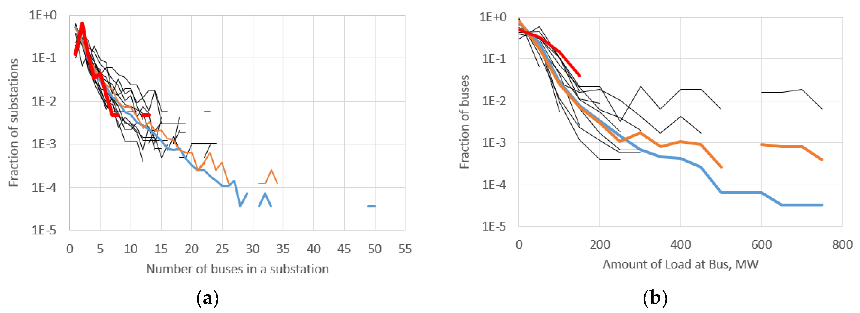
Table 6, along with
Figure 9 and
Figure 10, shows the validation of these two synthetic cases according to the criteria in this paper. These cases fully satisfy the metrics defined in this paper, which are derived from actual grid analysis. The table also shows where among the diversity of studied cases these synthetic ones lie. For example, while both cases have their distribution of generator capacities (metric 7) fully matching the realistic metric, they both share similarities with cases that model smaller generators more explicitly (over 30%), and are on opposite ends of the large generator spectrum (ACTIVSg200 has 6% of generators larger than 200 MW, ACTIVSg500 has 16%).

 ,
, 


