Optimal Voltage Control Using an Equivalent Model of a Low-Voltage Network Accommodating Inverter-Interfaced Distributed Generators

Abstract
:1. Introduction
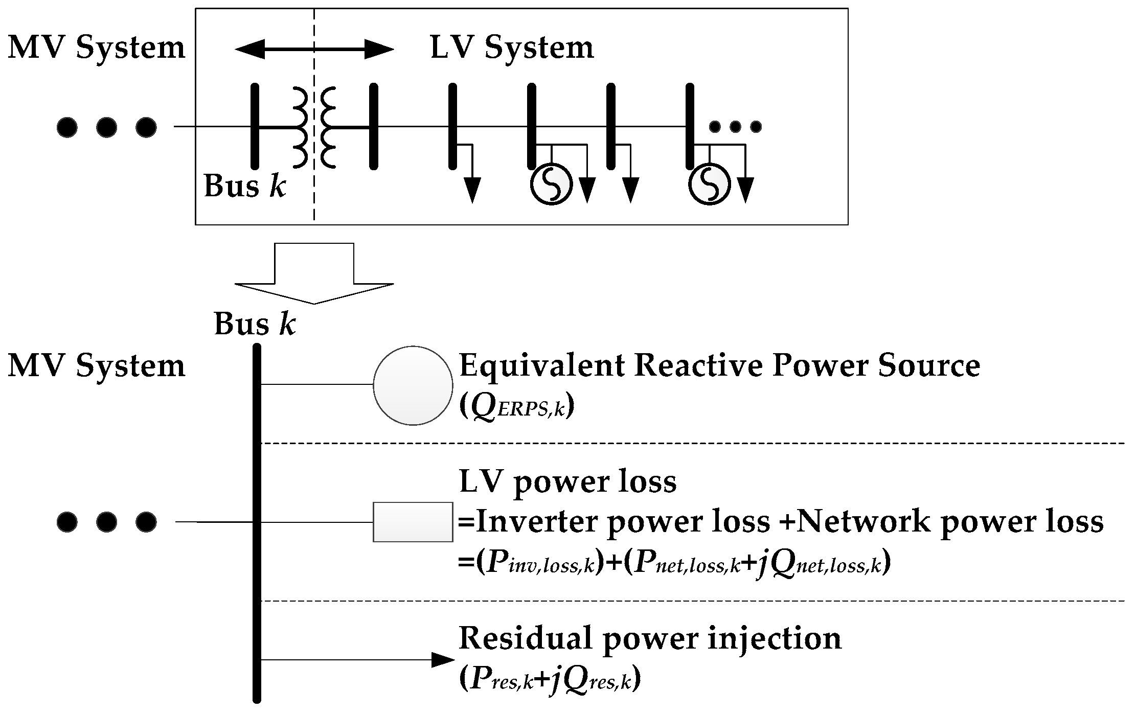
2. Equivalent Model for Low-Voltage Distribution System with Distributed Generators
2.1. Equivalent Reactive Power Source (ERPS)
2.2. Low-Voltage Power Loss
2.2.1. Inverter Power Loss
2.2.2. Network Power Loss
2.3. Residual Power Injection
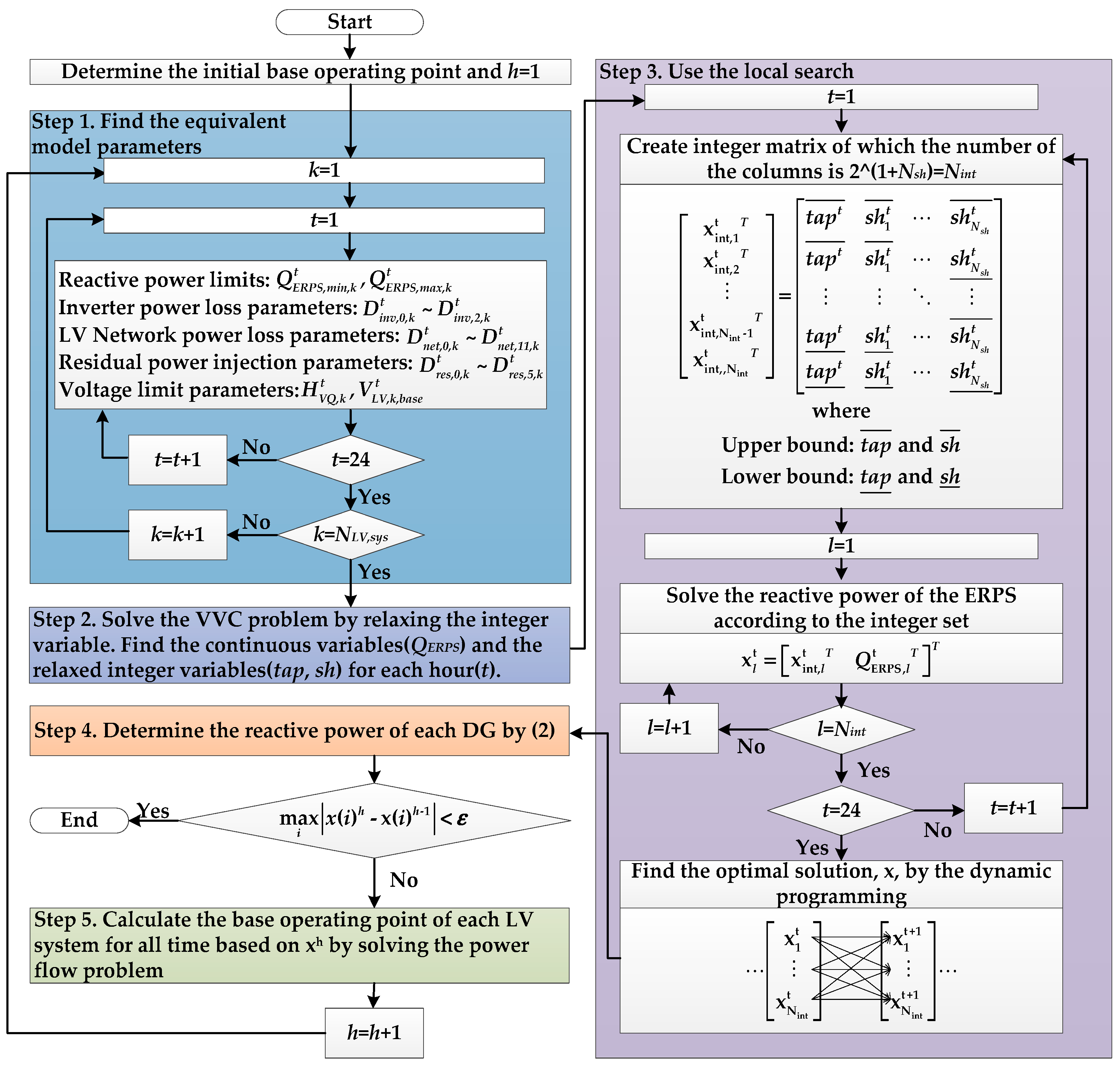
3. Application to Volt/Var Optimization Problem Formulation
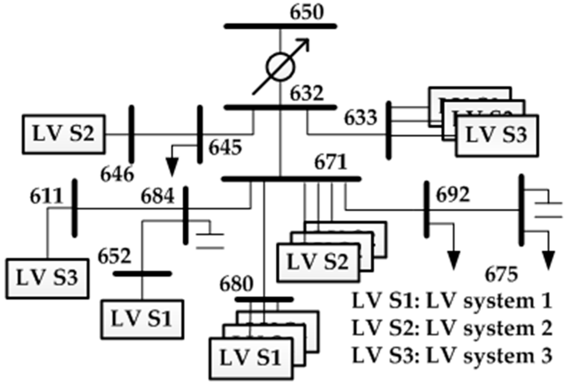
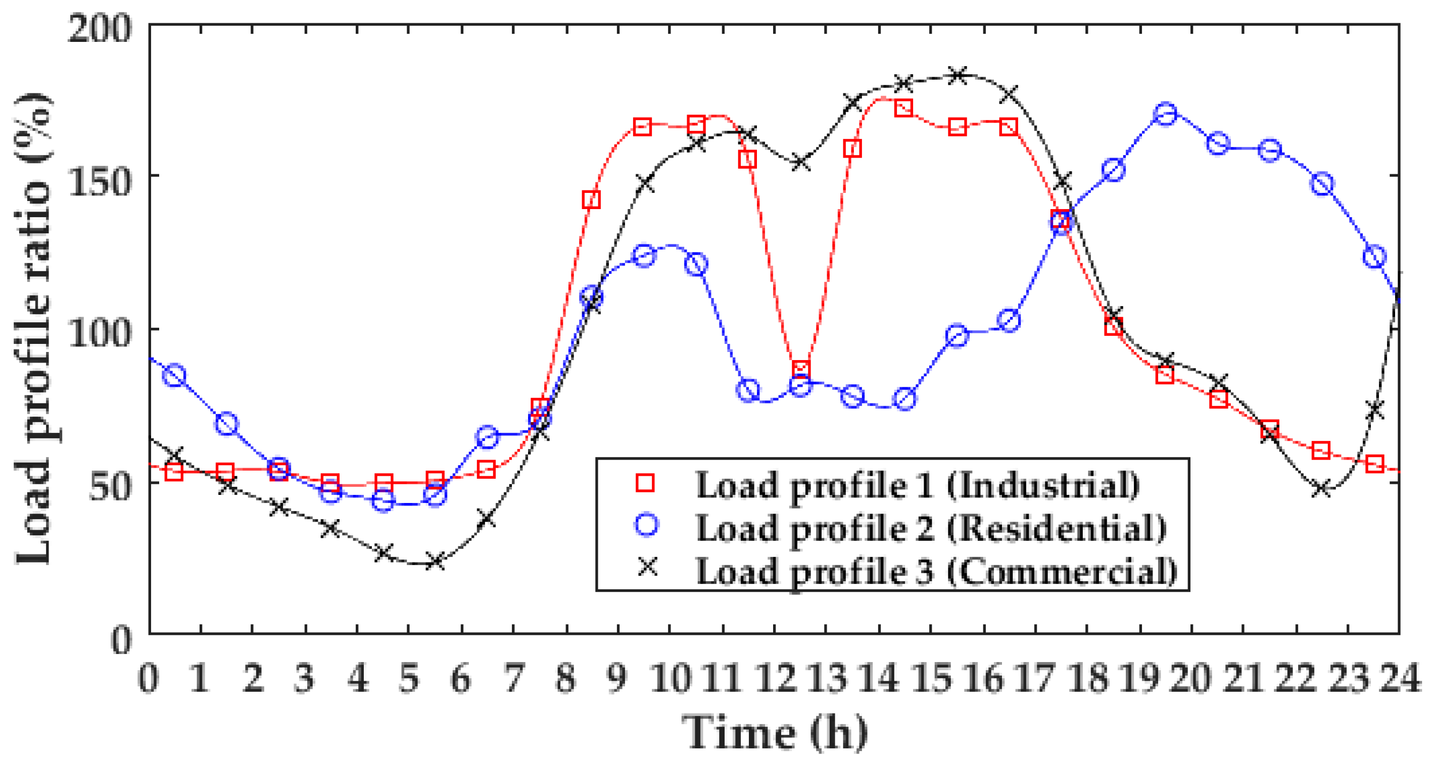
4. Case Study
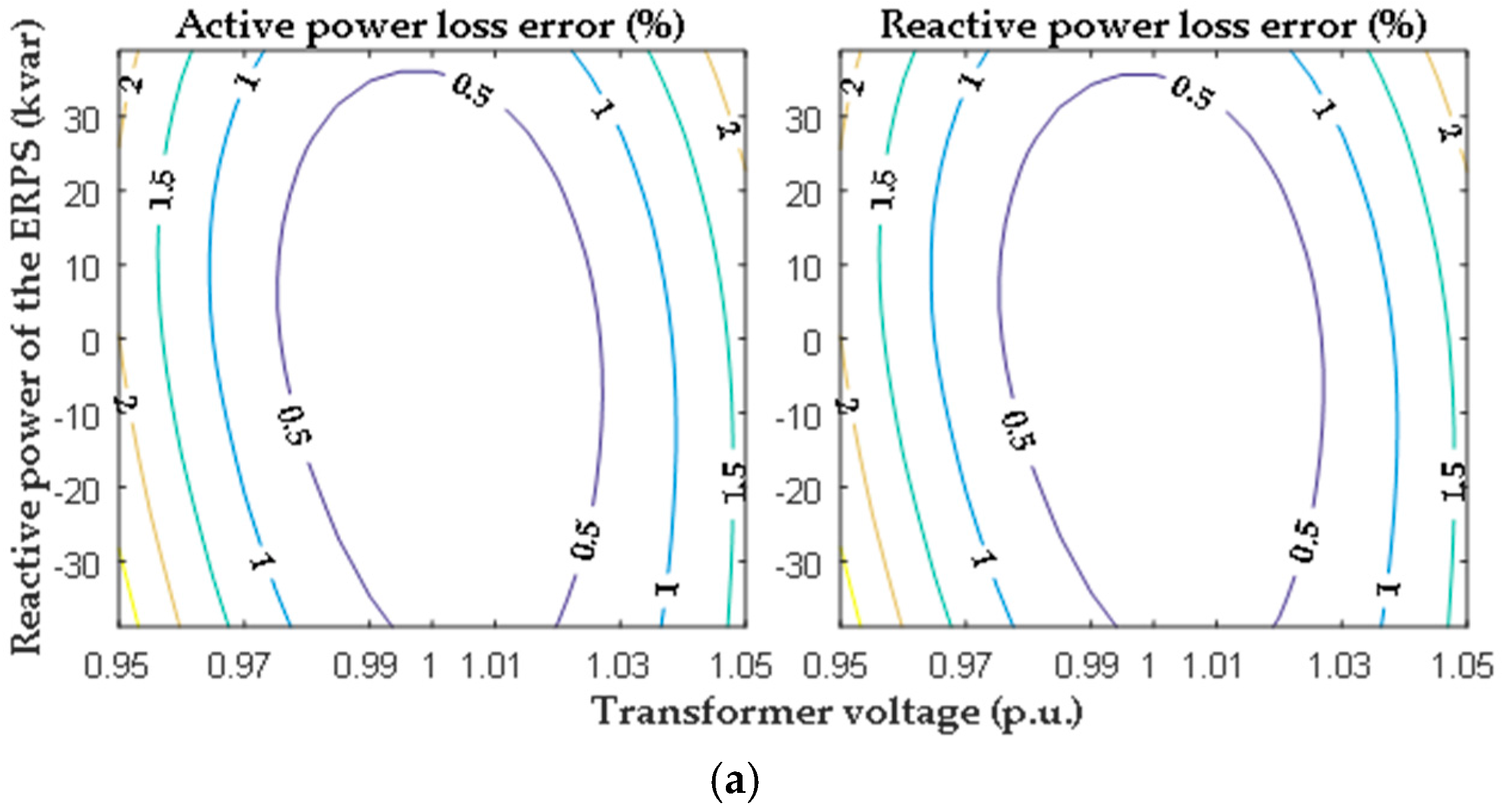
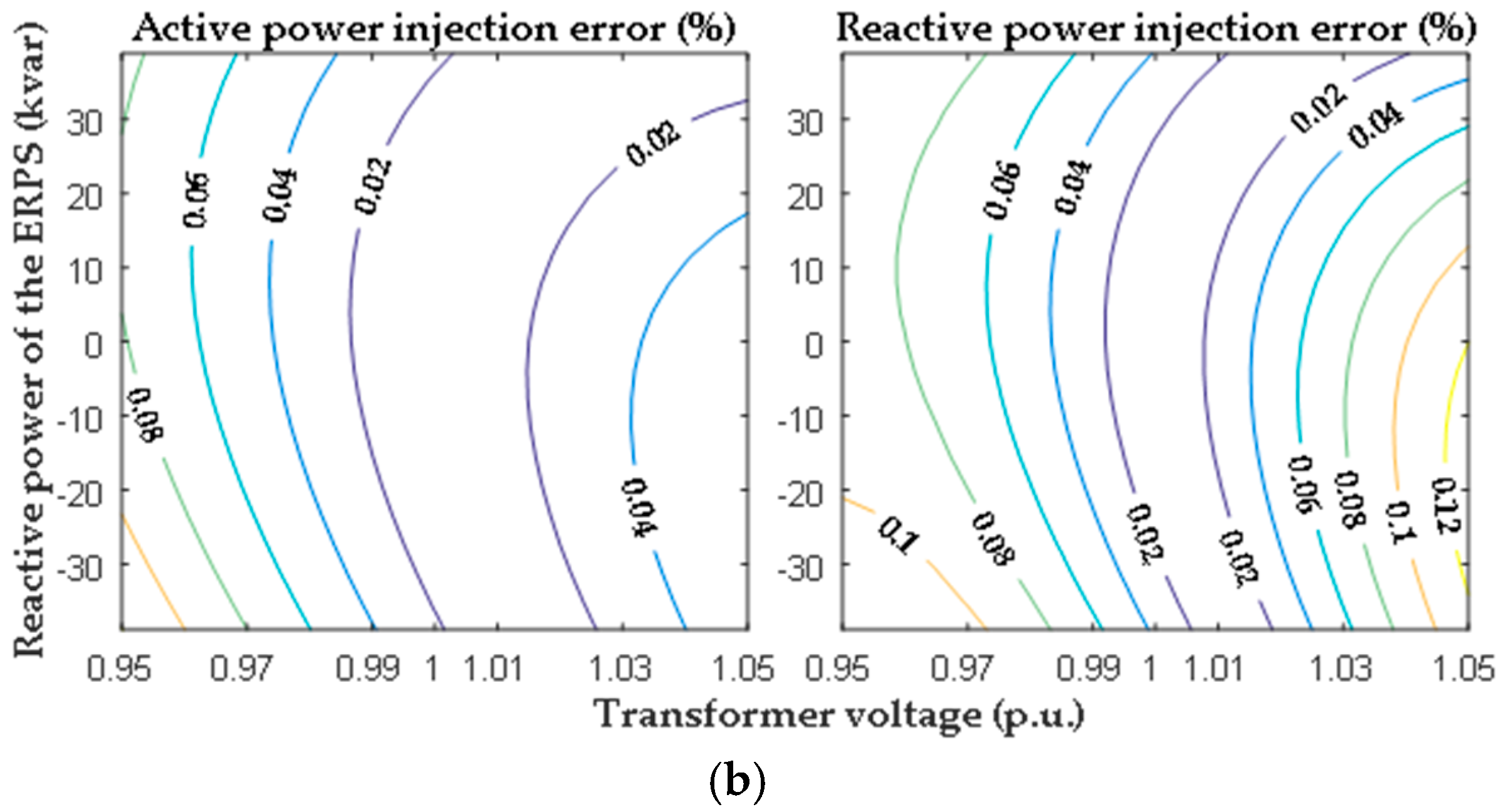
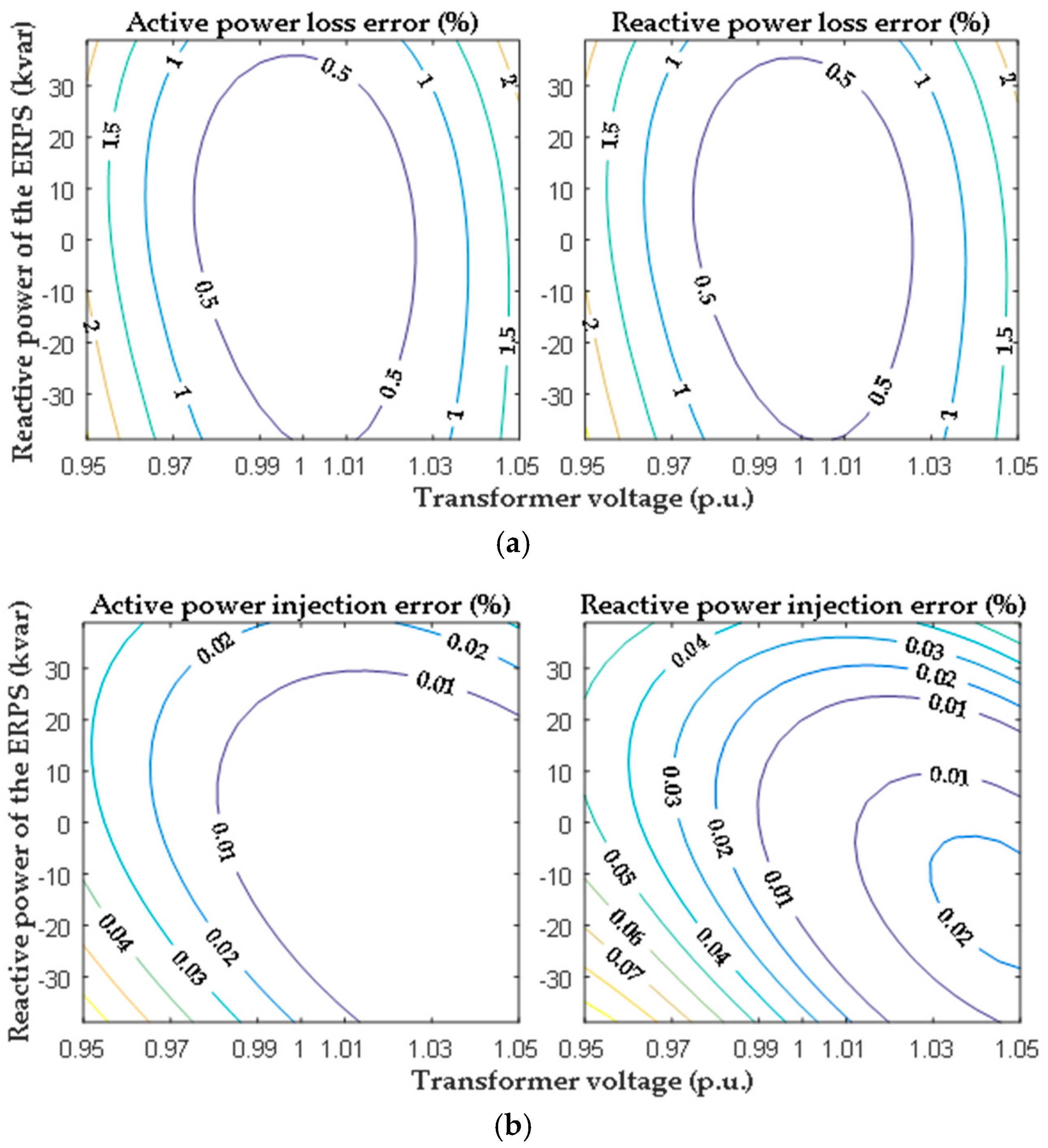
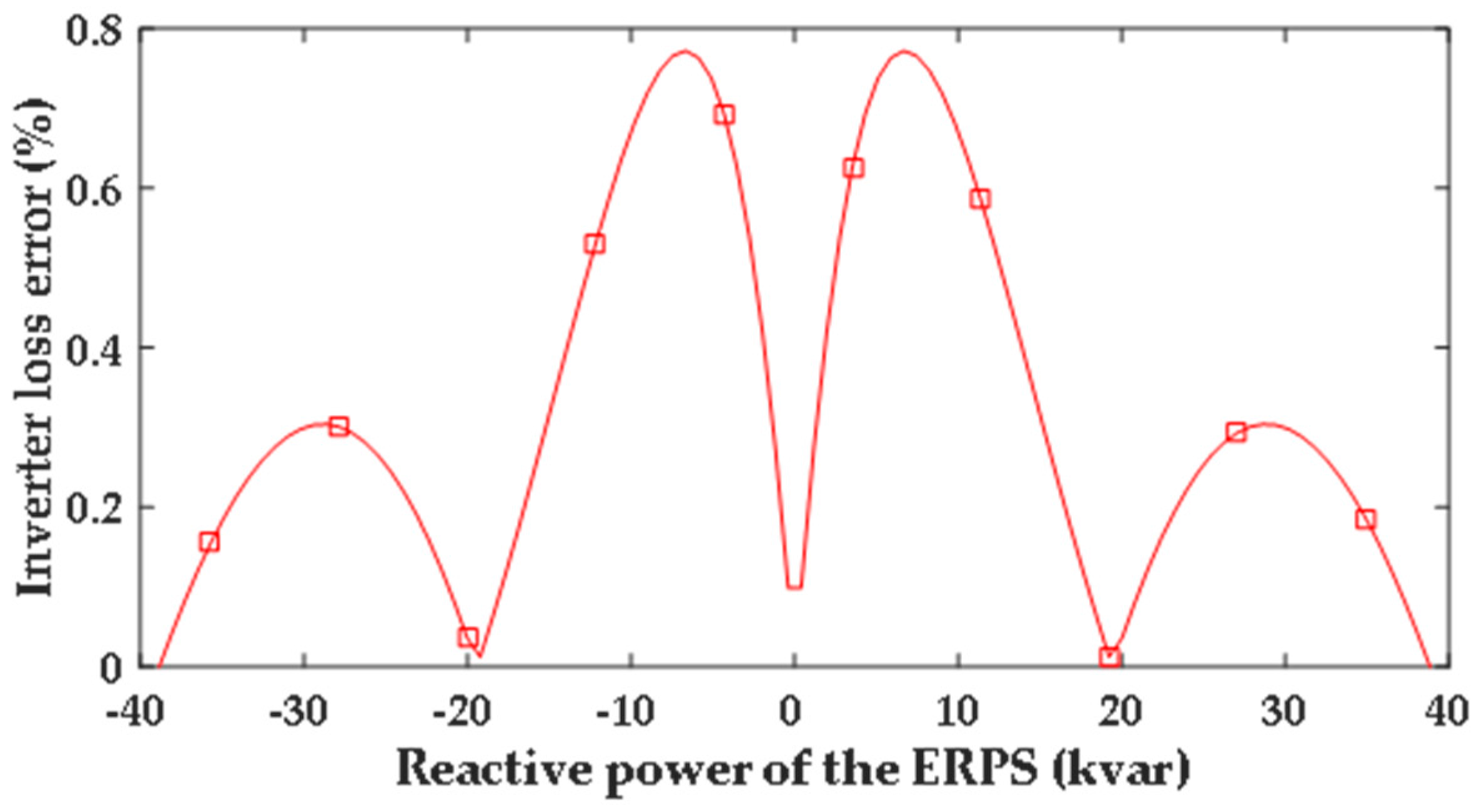
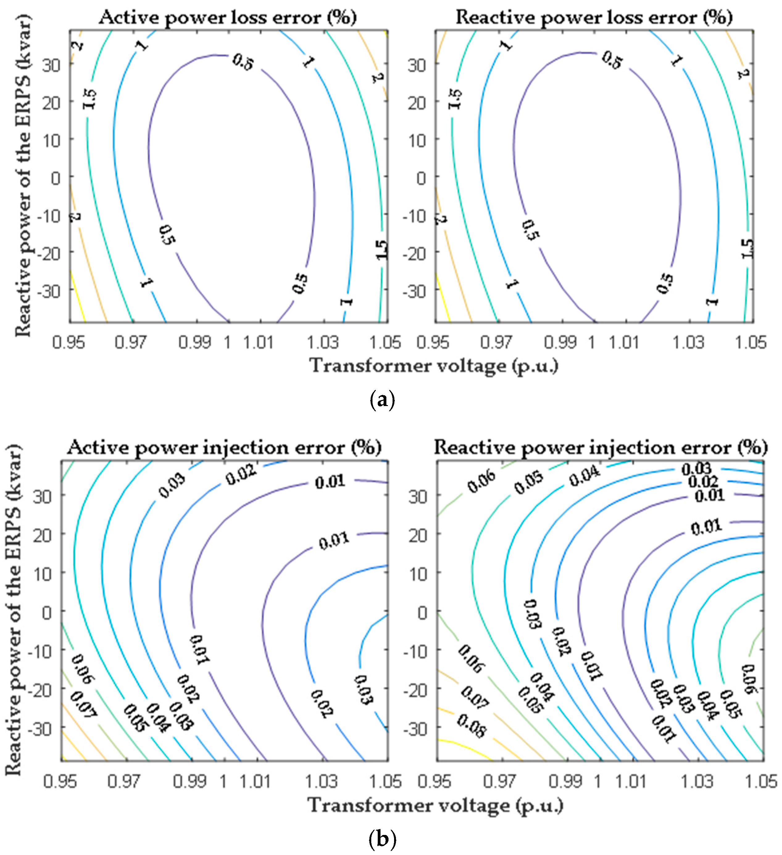
4.1. Accuracy of the Low-Voltage Power Loss Model
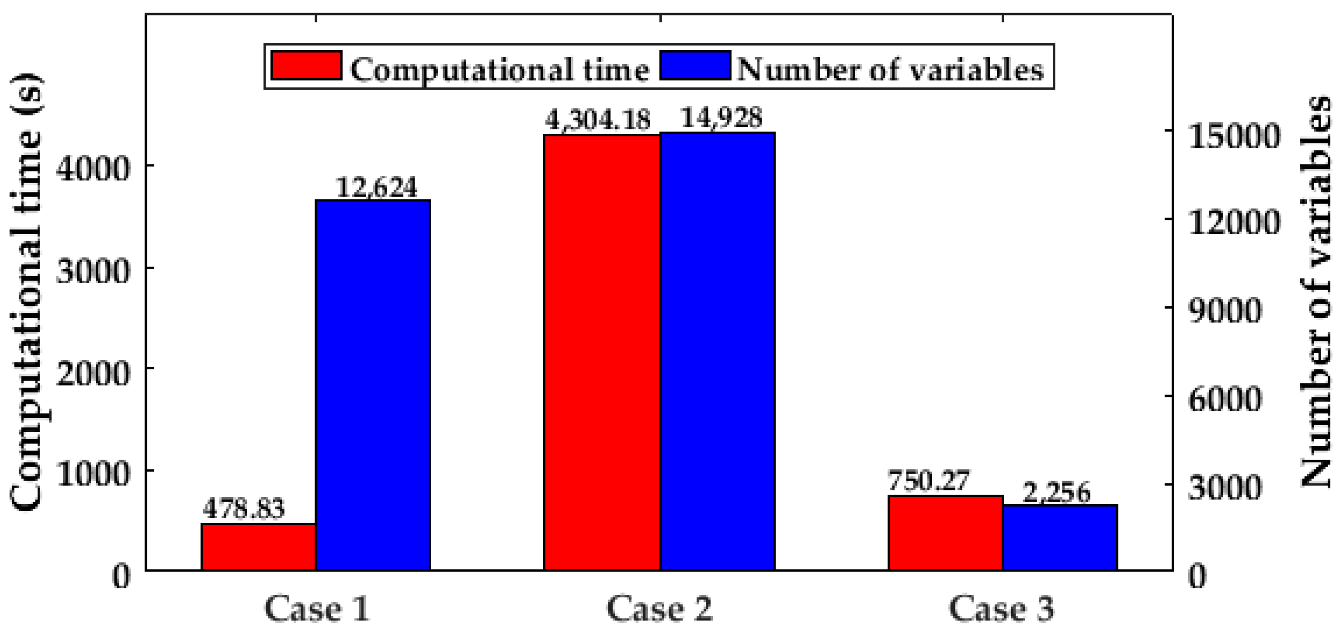
4.2. Effect on the Volt/Var Optimization
- Case 1: The DGs in the LV systems are not utilized for the VVO. Detailed models of the LV systems are used in the VVO.
- Case 2: The DGs in the LV systems are utilized for the VVO. Detailed models of the LV systems are used in the VVO. In other words, the reactive power outputs of the DGs are determined by solving a detailed optimal power flow problem, not by using Equation (2).
- Case 3: The DGs in the LV systems are utilized for the VVO. However, the proposed model is used in the VVO.
5. Conclusions
Author Contributions
Conflicts of Interest
Nomenclature
| Indices and subscripts | |
| k, n | Indices of the MV buses |
| i, m | Indices of the LV buses |
| l | Index of the integer variables |
| β | Index of the impedance-current-power (ZIP) coefficient |
| t | Index of the hours * |
| h | Index of the iterations * |
| base | Subscript for the base operating point |
| min, max | Subscripts for the minimum and maximum limits |
| Variables | |
| EMV(LV), θMV(LV), VMV(LV) | Voltage phasor, magnitude, and angle of each MV (LV) bus |
| PMV(LV), QMV(LV), SMV(LV) | Active, reactive, and complex power injection into each MV (LV) bus |
| PDG, QDG, SDG | Active, reactive, and complex power of each DG |
| PDG,inv | Actual active power of each DG excluding the inverter power loss |
| Srated | Rated capacity of the inverter of each DG |
| PLoad,QLoad | Active and reactive power of each load |
| PL,norm, QL,norm | Active and reactive power of each load when voltage = 1 p.u. |
| KP, KQ | ZIP coefficients for active and reactive powers |
| IMV(LV) | Injection current into each MV (LV) bus |
| Y1 | Self-admittance of an MV bus connected to an LV system |
| Y2 | Admittance between the MV bus and an LV system |
| Y3 | Admittance of an LV system |
| GMV, BMV | Conductance and susceptance of the MV system |
| QERPS | Aggregated reactive power of the DGs in an LV system |
| α | Ratio of QDG to QERPS |
| Pinv,loss | Aggregated inverter power loss of the DGs in an LV system |
| Pnet,loss, Qnet,loss, Snet,loss | Network active, reactive, and complex losses in an LV system |
| Pres, Qres | Residual active and reactive power injections in an LV system |
| tap | Tap position |
| sh | Number of unit capacitors connected to the MV feeders |
| wP, wtap, wsh | Cost weights of the objective function |
| HVQ | Voltage sensitivity with respect to the reactive powers of the ERPS |
| WVQ | Voltage sensitivity matrix with respect to the individual reactive powers of the DGs in an LV system |
| Nsh | Total number of shunt capacitors in an MV system |
| NLV,sys | Total number of LV systems in an MV system |
| NMV,Bus | Total number of MV buses |
| NLV,Bus | Total number of buses in the LV system connected to an MV bus |
| NLV,DG | Total number of DGs in the LV system connected to an MV bus |
| * Superscript index. | |
Appendix A. Inverter Power Loss
Appendix B. Voltage Magnitude Variations in the Low-Voltage System
Appendix C. Network Power Loss
Appendix D. Equivalent Model Error in Low-Voltage Systems 2 and 3

References
- Chiradeja, P.; Ramakumar, R. An approach to quantify the technical benefits of distributed generation. IEEE Trans. Energy Convers. 2004, 19, 764–773. [Google Scholar] [CrossRef]
- Keane, A.; Ochoa, L.F.; Vittal, E.; Dent, C.J.; Harrixon, G.P. Enhanced utilization of voltage control resources with distributed generation. IEEE Trans. Power Syst. 2011, 26, 252–260. [Google Scholar] [CrossRef] [Green Version]
- Carvalho, P.M.S.; Correia, P.F.; Ferreira, L.A.F.M. Distributed reactive power generation control for voltage rise mitigation in distribution networks. IEEE Trans. Power Syst. 2008, 23, 766–772. [Google Scholar] [CrossRef]
- Mohapatra, A.; Bijwe, P.R.; Panigrahi, B.K. An efficient hybrid approach for volt/var control in distribution systems. IEEE Trans. Power Deliv. 2014, 29, 1780–1788. [Google Scholar] [CrossRef]
- Kim, Y.J.; Ahn, S.J.; Hwang, P.I.; Pyo, G.C.; Moon, S.I. Coordinated control of a DG and voltage control devices using a dynamic programming algorithm. IEEE Trans. Power Syst. 2013, 28, 42–51. [Google Scholar] [CrossRef]
- Samimi, A.; Kazemi, A. A new approach to optimal allocation of reactive power ancillary service in distribution systems in the presence of distributed energy resources. Appl. Sci. 2015, 5, 1284–1309. [Google Scholar] [CrossRef]
- Hwang, P.I.; Moon, S.I.; Ahn, S.J. A conservation voltage reduction scheme for a distribution systems with intermittent distributed generators. Energies 2016, 9, 666. [Google Scholar] [CrossRef]
- Von Appen, J.; Braun, M.; Stetz, T.; Diwold, K.; Geibel, D. Time in the Sum: the challenge of high PV penetration in the German electric grid. IEEE Power Energy Mag. 2013, 11, 55–64. [Google Scholar] [CrossRef]
- Thomson, M.; Infield, D.G. Network power-flow analysis for a high penetration of distributed generation. IEEE Trans. Power Syst. 2007, 22, 1157–1162. [Google Scholar] [CrossRef] [Green Version]
- Trichakis, P.; Taylor, P.C.; Lyons, P.F.; Hair, R. Predicting the technical impacts of high level of small-scale embedded generators on low-voltage networks. IET Renew. Power Gener. 2008, 2, 249–262. [Google Scholar] [CrossRef]
- Braun, M.; Stetz, T.; Brundlinger, R.; Mayr, C.; Ogimoto, K.; Hatta, H.; Kobayashi, H.; Kroposki, B.; Mather, B.; Coddington, M.; et al. Is the distribution grid ready to accept large-scale photovoltaic deployment? State of art, progress, and future prospects. Prog. Photovolt. 2012, 20, 681–697. [Google Scholar] [CrossRef]
- Samadi, A.; Eriksson, R.; Soder, L.; Rawn, B.G.; Boemer, J.C. Coordinated active power dependent voltage regulation in distribution grids with PV systems. IEEE Trans. Power Deliv. 2014, 29, 1454–1464. [Google Scholar] [CrossRef]
- Niknam, T.; Zare, M.; Aghaei, J. Scenario-based multiobjective volt/var control in distribution networks including renewable energy sources. IEEE Trans. Power Deliv. 2012, 27, 2004–2019. [Google Scholar] [CrossRef]
- Wang, Z.; Wang, J.; Chen, B.; Begovic, M.M.; He, Y. MPC-based voltage/var optimization for distribution circuits with distributed generators and exponential load models. IEEE Trans. Smart Grid 2014, 5, 2412–2420. [Google Scholar] [CrossRef]
- Zhang, C.; Chen, H.; Ngan, H. Reactive power optimisation considering wind farms based on an optimal scenario method. IET Gener. Trans. Distrib. 2016, 10, 3736–3744. [Google Scholar] [CrossRef]
- Ward, J.B. Equivalent circuits for power flow studies. AIEE Trans. 1949, 68, 373–382. [Google Scholar] [CrossRef]
- Liacco, T.E.D.; Savulescu, S.C.; Ramaro, K.A. An on-line topological equivalent of a power system. IEEE Trans. Power Appar. Syst. 1978, PAS-97, 1550–1563. [Google Scholar] [CrossRef]
- Collin, A.J.; Acosta, J.L.; Hernando-Gil, I.; Djokic, S.Z. An 11kV steady state residential aggregate load model. Part 2: Microgeneration and demand-side management. In Proceedings of the 2011 IEEE Trondheim PowerTech, Trondheim, Norway, 19–23 June 2011. [Google Scholar]
- Collin, A.J.; Tsagarakis, G.; Kiprakis, A.E.; McLaughlin, S. Development of low-voltage load models for the residential load sector. IEEE Trans. Power Syst. 2014, 29, 2180–2188. [Google Scholar] [CrossRef]
- Di Fazio, A.R.; Russo, M.; Valeri, S.; De Santis, M. Sensitivity-based model of low voltage distribution systems with distributed energy resources. Energies 2016, 9, 801. [Google Scholar] [CrossRef]
- Samadi, A.; Soder, L.; Shayestech, E.; Eriksson, R. Static equivalent of distribution grids with high penetration of PV systems. IEEE Trans. Smart Grid 2015, 6, 1763–1774. [Google Scholar] [CrossRef]
- Madureira, A.G.; Lopes, J.A.P. Coordinated voltage support in distribution networks with distributed generation and microgrids. IET Renew. Power Gener. 2009, 3, 439–454. [Google Scholar] [CrossRef]
- Hemmati, R.; Hooshmand, R.A.; Khodabakhshian, A. State-of-the-art of transmission expansion planning: Comprehensive review. Renew. Sustain. Energy Rev. 2013, 23, 312–319. [Google Scholar] [CrossRef]
- Su, X.; Masoum, M.A.S.; Wolfs, P.J. Optimal PV inverter reactive power control and real power curtailment to improve performance of unbalanced four-wire LV distribution networks. IEEE Trans. Sustain. Energy 2014, 5, 967–977. [Google Scholar] [CrossRef]
- Braun, M. Reactive power supplied by PV inverters-cost benefit analysis. In Proceedings of the 22nd European Photovoltaic Solar Energy Conference and Exhibition, Milan, Italy, 3–7 September 2007. [Google Scholar]
- El-Aal, M.A.A. Modelling and Simulation of a Photovoltaic Fuel Cell Hybrid System. Ph.D. Thesis, University of Kassel, Kassel, Germany, 2005. [Google Scholar]
- Chapra, S.C.; Canale, R.P. Numerical Methods for Engineers, 6th ed.; McGraw-Hill: Boston, MA, USA, 2011; pp. 500–501. [Google Scholar]
- Kundur, P. Power System Stability and Control; McGraw-Hill: New York, NY, USA, 1994; p. 273. [Google Scholar]
- Bokhari, A.; Alkan, A.; Dogan, R.; Auilo, M.D.; Leon, F.; Czarkowski, D.; Zabar, Z.; Birenbaum, L.; Noel, A.; Uosef, R.E. Experimental determination of the ZIP coefficients for modern residential, commercial, and industrial loads. IEEE Trans. Power Deliv. 2014, 29, 1372–1381. [Google Scholar] [CrossRef]
- Azzouz, M.A.; Farag, H.E.; El-Saadany, E.F. Real-time fuzzy voltage regulation for distribution networks incorporating high penetration of renewables sources. IEEE Syst. J. 2014, PP, 1–10. [Google Scholar] [CrossRef]
- Bergen, R.; Vittal, V. Power System Analysis, 2nd ed.; Prentice Hall: Upper Saddle River, NJ, USA, 2006; p. 352. [Google Scholar]
- Wood, A.J.; Wollenberg, B.F. Power Generation, Operation, and Control, 3rd ed.; John Wiley & Sons: New York, NY, USA, 2013; p. 105. [Google Scholar]
- Roytelman, I.; Ganesan, V. Coordinated local and centralized control in distribution management systems. IEEE Trans. Power Deliv. 2000, 15, 718–724. [Google Scholar] [CrossRef]
- Zhu, J. Optimization of Power System Operation; John Wiley & Sons: Hoboken, NJ, USA, 2009; p. 409. [Google Scholar]
- Paudyal, S.; Canizares, C.A.; Bhattacharya, K. Optimal operation of distribution feeders in smart grids. IEEE Trans. Ind. Electron. 2011, 58, 4495–4503. [Google Scholar] [CrossRef]
- Boyd, S.; Vandenberghe, L. Convex Optimization; Cambridge University Press: Cambridge, UK, 2004; pp. 143–150. [Google Scholar]


| Bus No. | PDG (kW) | cinv,0 | cinv,1 | cinv,2 |
|---|---|---|---|---|
| 3 | 1.0 | 3.5 × 10⁻³ | 5.0 × 10⁻³ | 1.00 × 10⁻² |
| 4 | 1.6 | 3.5 × 10⁻³ | 5.0 × 10⁻³ | 1.00 × 10⁻² |
| 5 | 2.2 | 3.7 × 10⁻³ | 5.2 × 10⁻³ | 1.05 × 10⁻² |
| 6 | 2.8 | 3.7 × 10⁻³ | 5.2 × 10⁻³ | 1.05 × 10⁻² |
| 7 | 3.4 | 3.9 × 10⁻³ | 5.4 × 10⁻³ | 1.1 × 10⁻² |
| 8 | 4.0 | 3.9 × 10⁻³ | 5.4 × 10⁻³ | 1.1 × 10⁻² |
| 9 | 4.6 | 4.1 × 10⁻³ | 5.6 × 10⁻³ | 1.15 × 10⁻² |
| 10 | 5.2 | 4.1 × 10⁻³ | 5.6 × 10⁻³ | 1.15 × 10⁻² |
| Type | KP,2 | KP,1 | KP,0 | KQ,2 | KQ,1 | KQ,0 |
|---|---|---|---|---|---|---|
| 1 1 | 1.21 | −1.61 | 1.4 | 4.35 | −7.08 | 3.73 |
| 2 2 | 1.5 | −2.31 | 1.81 | 7.41 | −11.97 | 5.56 |
| 3 3 | 0.4 | −0.41 | 1.01 | 4.43 | −7.98 | 4.55 |
| Bus No. | Phase | Active Power, PL,norm (kW) | Reactive Power, QL,norm (kvar) | Load Profile |
|---|---|---|---|---|
| 633 | A | 105 (7.5 *) | 61 (4.4 *) | 1 |
| B | 69 (4.9 *) | 40 (2.9 *) | 1 | |
| C | 69 (4.9 *) | 40 (2.9 *) | 1 | |
| 645 | B | 131 | 76 | 2 |
| 646 | B | 119 (7.4 *) | 69 (4.3 *) | 2 |
| 671 | A | 99 (6.2 *) | 57 (3.6 *) | 2 |
| B | 99 (6.2 *) | 57 (3.6 *) | 2 | |
| C | 99 (6.2 *) | 57 (3.6 *) | 2 | |
| 692 | A | 65 | 38 | 3 |
| B | 65 | 38 | 3 | |
| C | 65 | 38 | 3 | |
| 675 | A | 174 | 101 | 1 |
| B | 131 | 76 | 1 | |
| C | 184 | 107 | 1 | |
| 680 | A | 99 (6.6 *) | 57 (3.8 *) | 3 |
| B | 111 (7.4 *) | 64 (4.3 *) | 3 | |
| C | 105 (7.0 *) | 61 (4.1 *) | 3 | |
| 684 | A | 65 | 38 | 1 |
| C | 65 | 38 | 1 | |
| 652 | A | 73 (4.9 *) | 42 (2.8 *) | 2 |
| 611 | C | 86 (6.1 *) | 50 (3.6 *) | 2 |
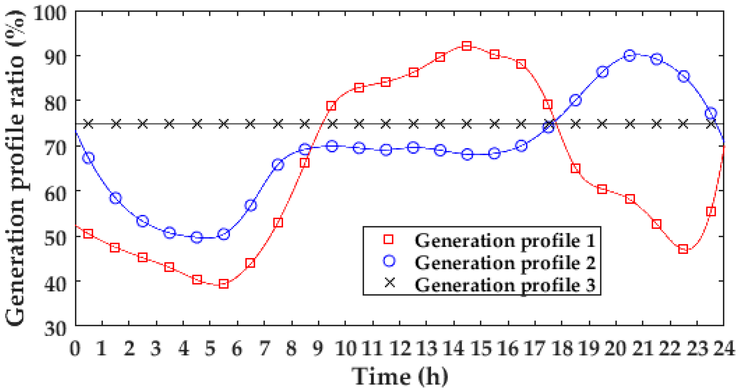
| Bus No. | DG Capacity * | Generation Profile | ||
|---|---|---|---|---|
| 652, 680 | 120% | 1 | ||
| 671, 646 | 80% | 2 | ||
| 633, 611 | 40% | 3 | ||
| Inverter power loss constants | cinv,0 | cinv,1 | cinv,2 | |
| 3.5 × 10⁻³ | 5.0 × 10⁻³ | 1.00 × 10⁻² | ||
| Parameters | Case 1 | Case 2 | Case 3 | |
|---|---|---|---|---|
| MV network active power loss (kWh) | 340 | 319 | 319 | |
| LV network active power loss (kWh) | 915 | 744 | 745 | |
| Inverter active power loss (kWh) | 137 | 174 | 175 | |
| Total active power loss (kWh) | 1392 | 1237 | 1239 | |
| Number of OLTC operations | 8 | 2 | 2 | |
| Number of shunt capacitor operations | 675A | 4 | 2 | 2 |
| 675B | 0 | 2 | 2 | |
| 675C | 2 | 2 | 2 | |
| 684A | 2 | 0 | 0 | |
| 684C | 2 | 0 | 0 | |
| Total number of switching operations | 18 | 8 | 8 | |
© 2017 by the authors. Licensee MDPI, Basel, Switzerland. This article is an open access article distributed under the terms and conditions of the Creative Commons Attribution (CC BY) license (http://creativecommons.org/licenses/by/4.0/).
Share and Cite
Jeong, M.-G.; Kim, Y.-J.; Moon, S.-I.; Hwang, P.-I. Optimal Voltage Control Using an Equivalent Model of a Low-Voltage Network Accommodating Inverter-Interfaced Distributed Generators. Energies 2017, 10, 1180. https://doi.org/10.3390/en10081180
Jeong M-G, Kim Y-J, Moon S-I, Hwang P-I. Optimal Voltage Control Using an Equivalent Model of a Low-Voltage Network Accommodating Inverter-Interfaced Distributed Generators. Energies. 2017; 10(8):1180. https://doi.org/10.3390/en10081180
Chicago/Turabian StyleJeong, Mu-Gu, Young-Jin Kim, Seung-Il Moon, and Pyeong-Ik Hwang. 2017. "Optimal Voltage Control Using an Equivalent Model of a Low-Voltage Network Accommodating Inverter-Interfaced Distributed Generators" Energies 10, no. 8: 1180. https://doi.org/10.3390/en10081180