Short-Term Load Forecasting Using EMD-LSTM Neural Networks with a Xgboost Algorithm for Feature Importance Evaluation

Abstract
:1. Introduction
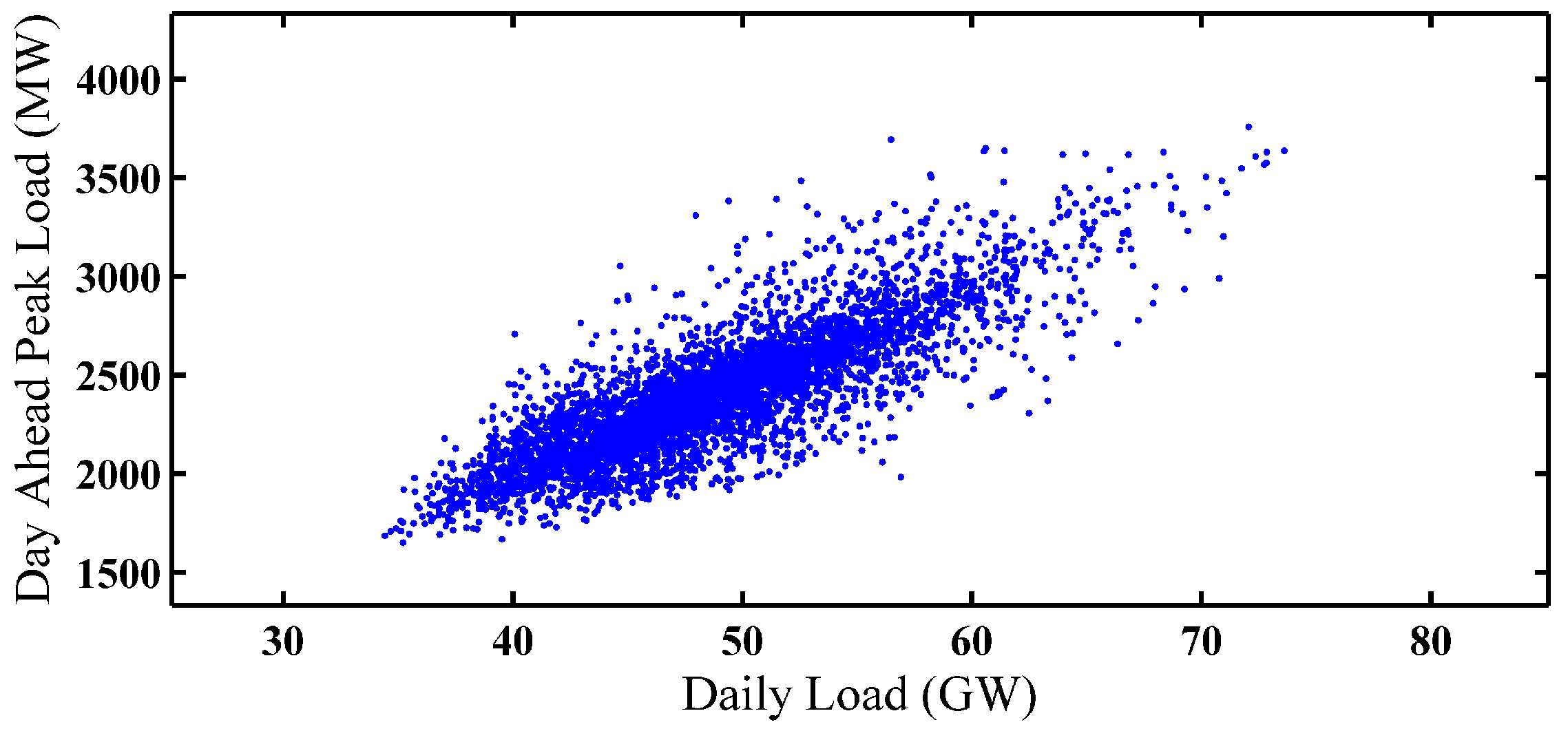
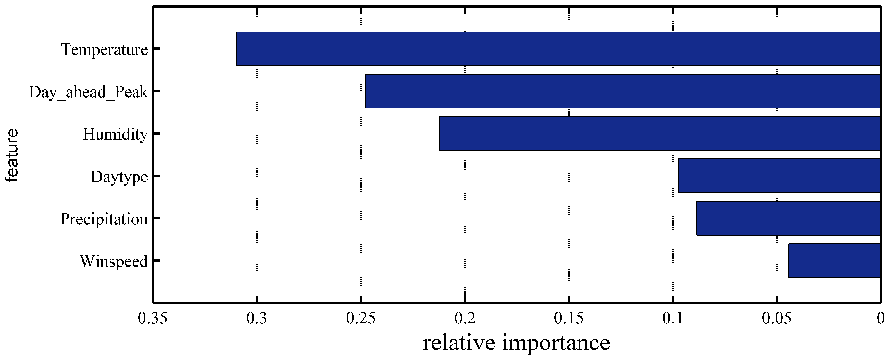
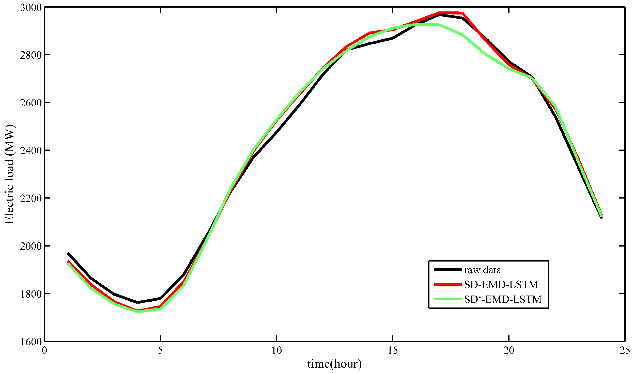
- Although the temperature, humidity, and day type have been extensively used as input features in STLF, we also recognize that STLF is sensitive to the day-ahead peak load, which has to be a supplemental input feature to the SD selection and LSTM training processes.
- Extending from our previous work on data analysis, we independently learned the feature candidate weights for the SD selection framework based on the Xgboost algorithm to overcome the dimensionality limitation in clustering. Thus, the proposed Xgboost-based k-means framework can deal with the SD selection tasks beyond pure clustering.
- Numerical testing demonstrates that data decomposition-based LSTM neural networks can outperform most of the well-established forecasting methods in the longer-horizon load forecasting problem.
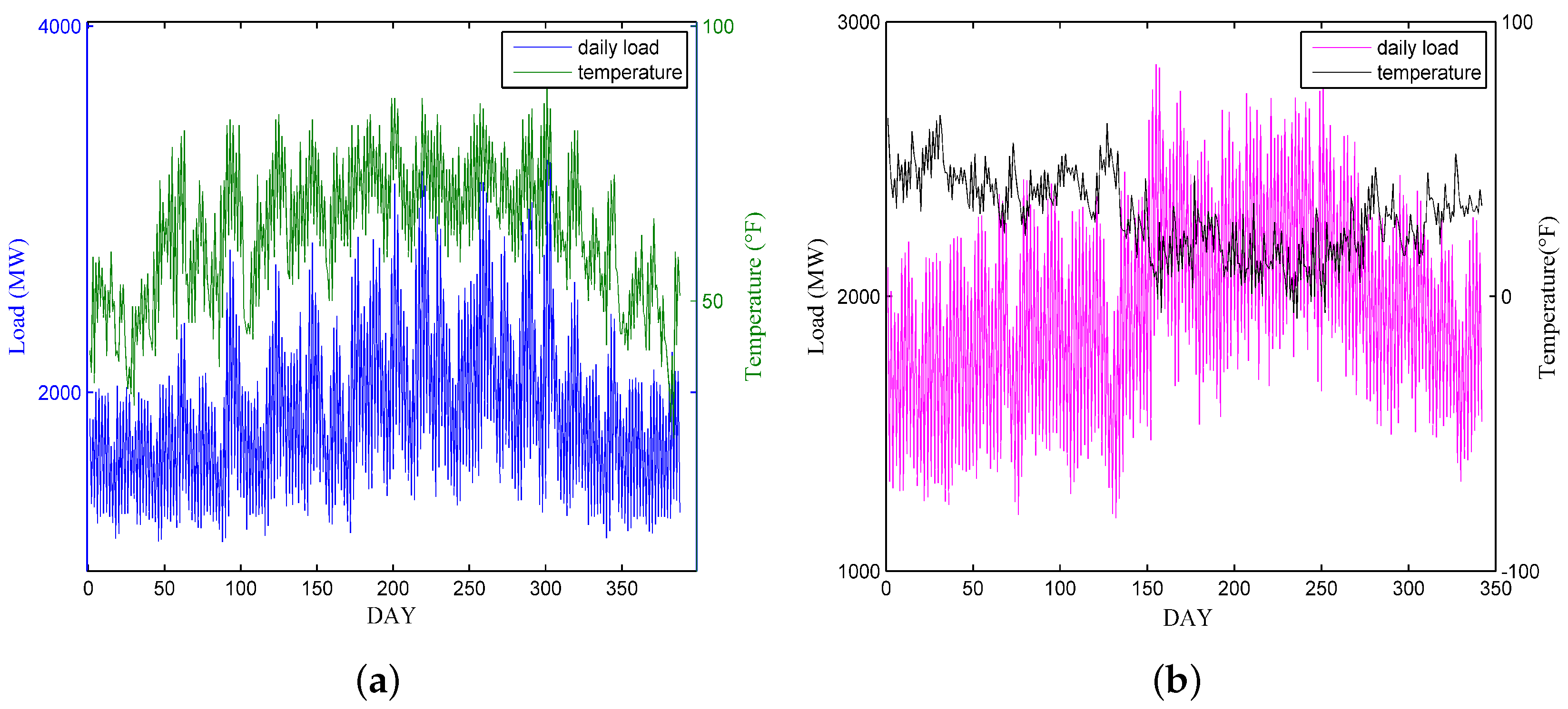
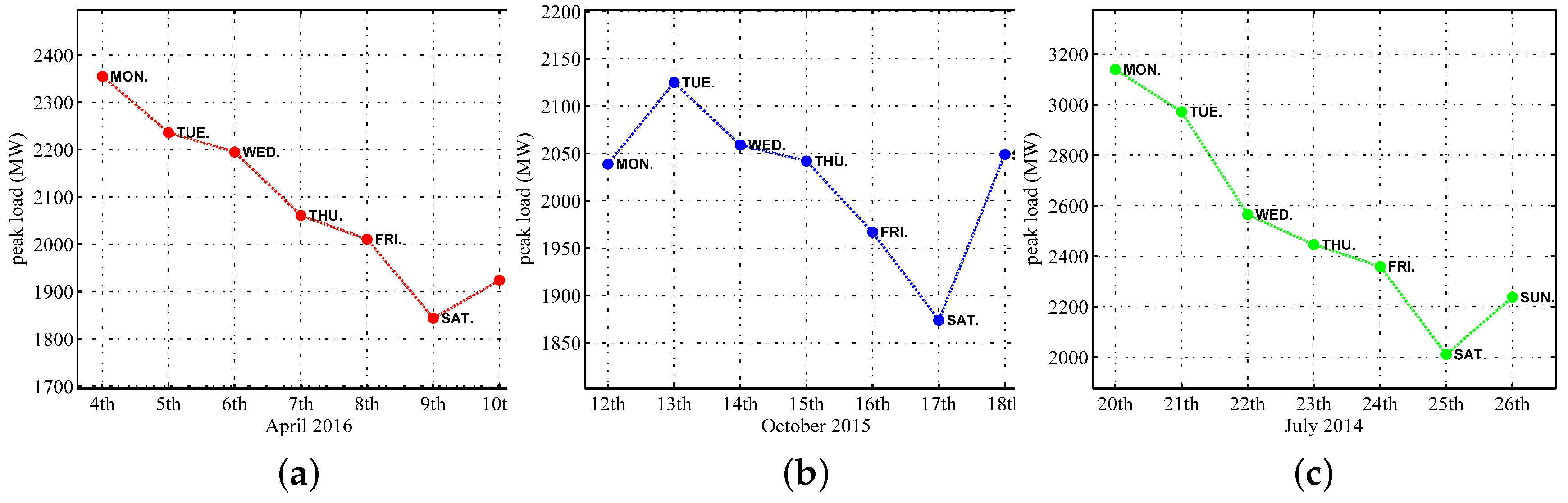
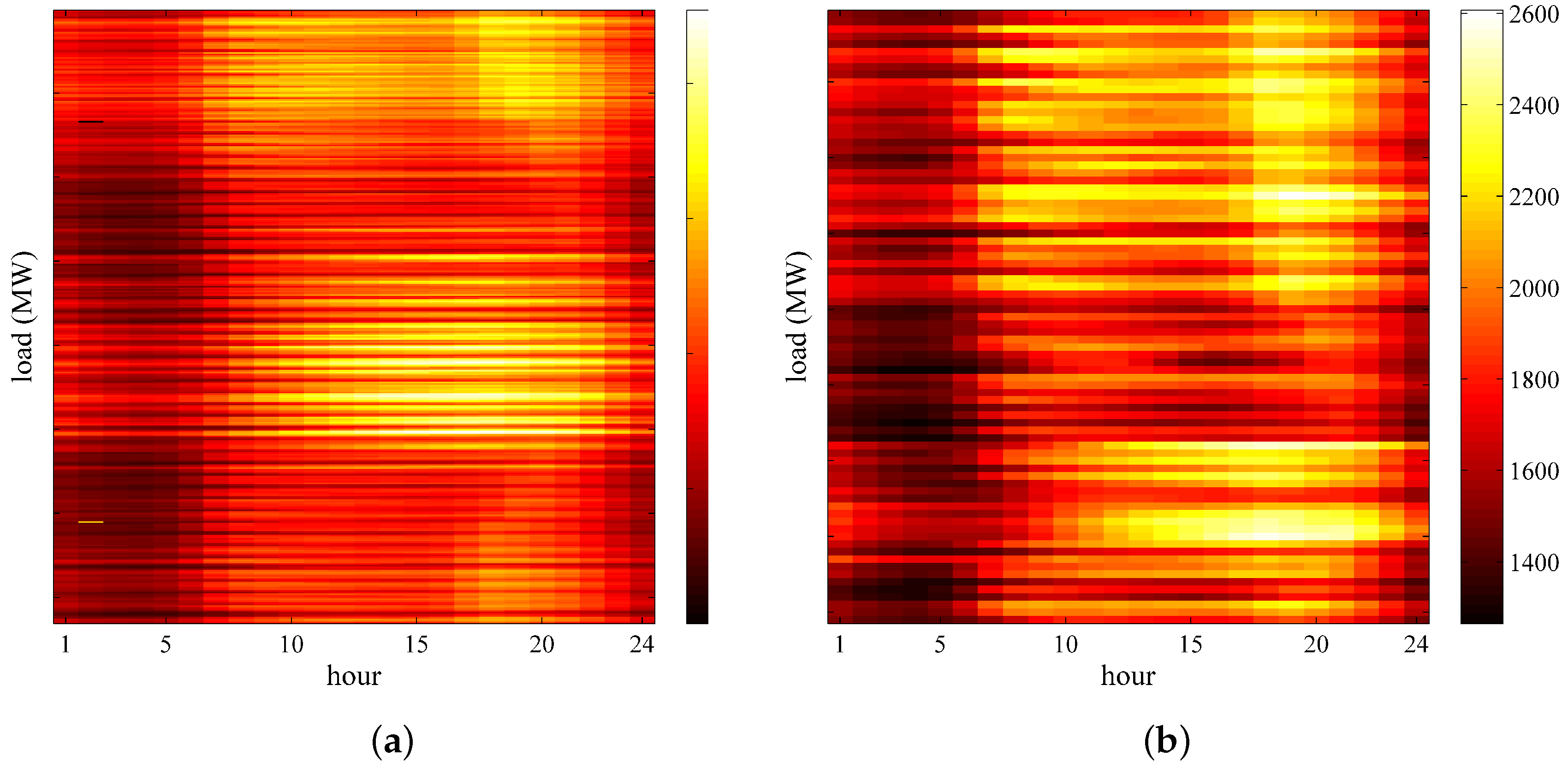
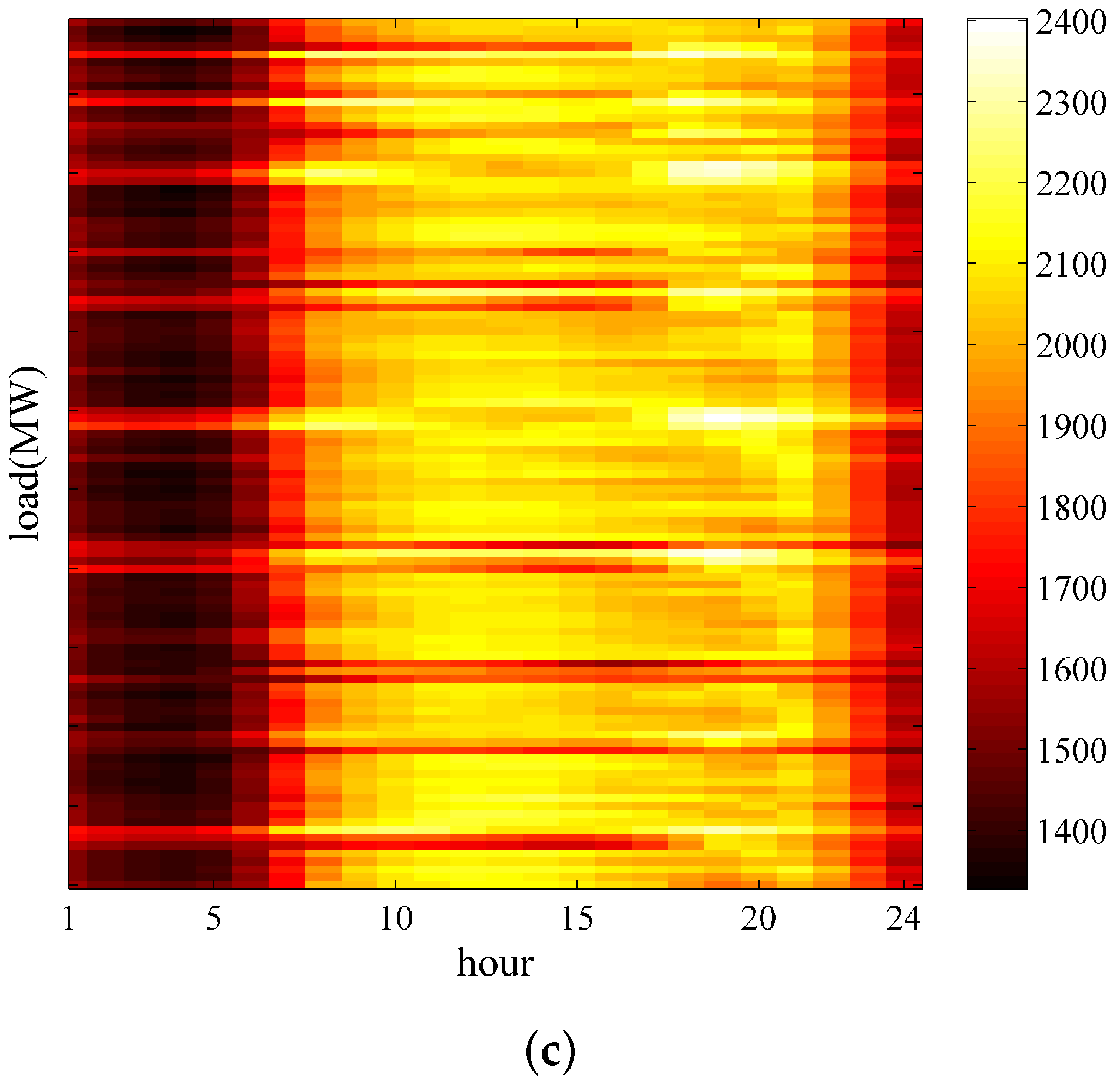
2. Data Analysis
3. Similar Day Selection: Improved K-Means with Extreme Gradient Boosting
3.1. Feature-Weight Learning Algorithm: Extreme Gradient Boosting
3.2. K-Means Clustering Based on Feature-Weight
- Given a data set and an integer value K. The data set is normalized as follows:where and denote the minimum and maximum values, respectively, of each input factor.
- The forecasting day is selected as the first center
- The next center is selected, where is the farthest point from the previously selected cluster centers . Steps 2 and 3 are repeated until the K centers have been identified.
- The feature weights are calculated using the Xgboost algorithm. Thereafter, the weights are attributed to each feature, thereby providing them with different levels of importance. Let be the weight associated with the feature p. The norm is presented as follows.(1) Each data point is assigned to the nearest cluster.(2) The clusters are updated by recalculating the cluster centroid. The algorithm repeatedly executes (1) and (2) until convergence is reached.
4. LSTM with Empirical Mode Decomposition
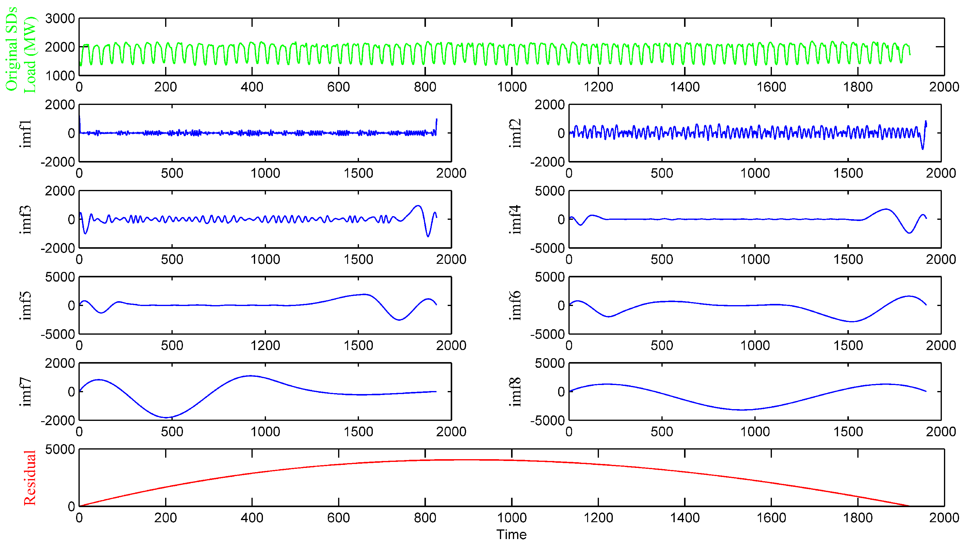
4.1. Empirical Mode Decomposition
- For a set of data sequences, the number of extremal points must be equal to the number of zero crossings or, at most, differ by one.
- For any point, the mean value of the envelope of the local maxima and local minima must be zero.
- Identify all the maxima and minima of signal .
- Through the cubic spline interpolation fitting out the upper envelope and lower envelope of signal . The mean of the two envelopes can be the average envelope curve :
- Subtraction of m from to obtain an IMF candidate :
- If does not satisfy the two conditions of the IMF, then it should take as original signal and repeat above calculate k times. At this point, could be as shown in Equation (7):and present the signal after shifting times and k times,respectively. is the average envelope of
- If satisfies the conditions of the IMF, define as . Standard deviation is defined by Equation (8):
- Subtraction of from to obtain new signal
- Repeat previous steps 1 to 6 until the cannot be decomposed into the IMF. is the residual of the original data . Finally, the original signal can be presented as a collection of n components and a residual :
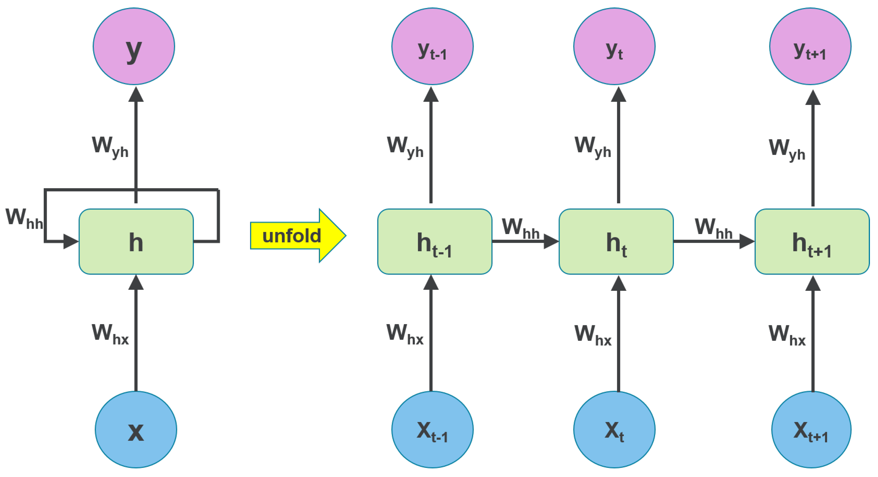
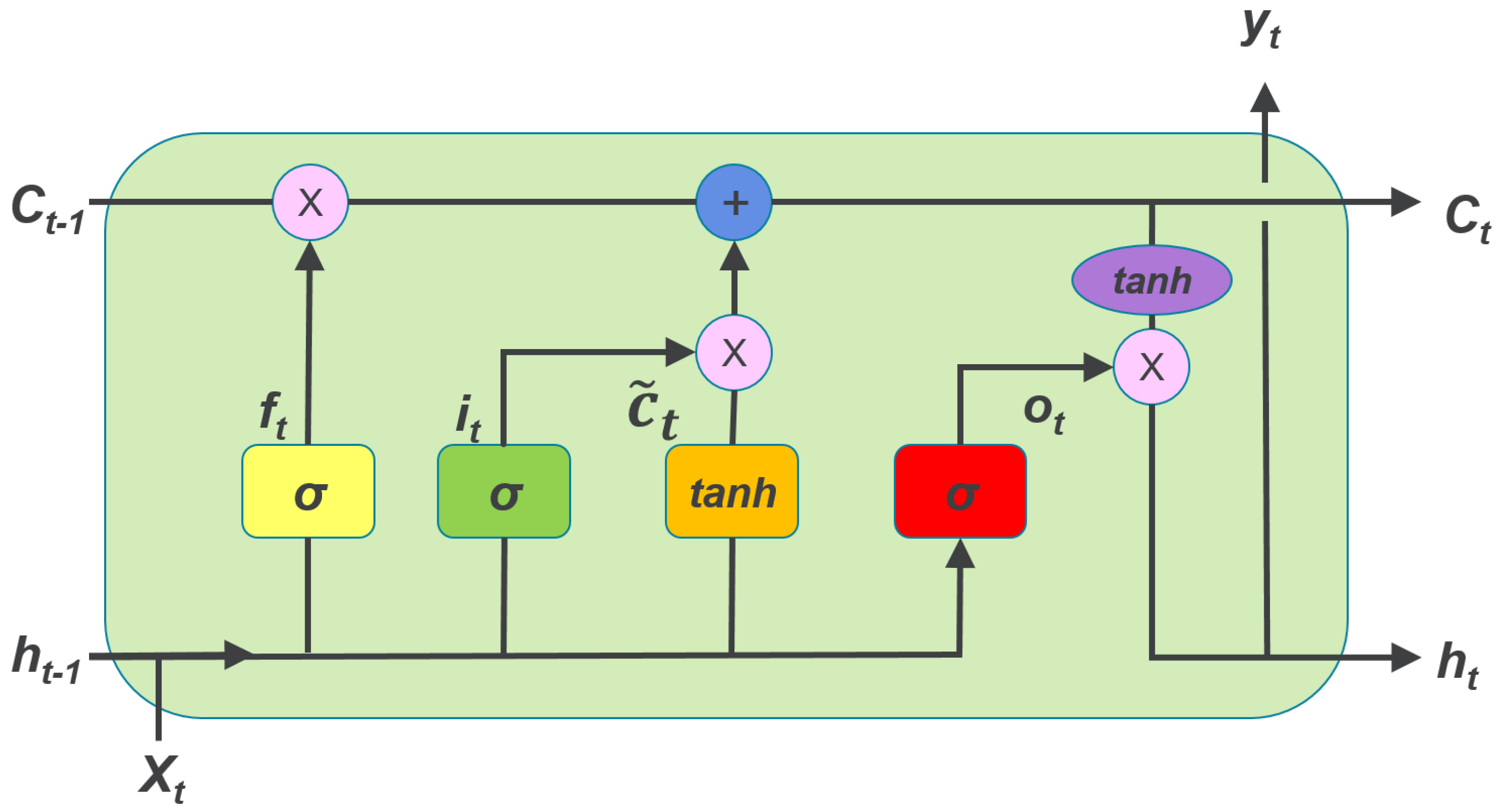
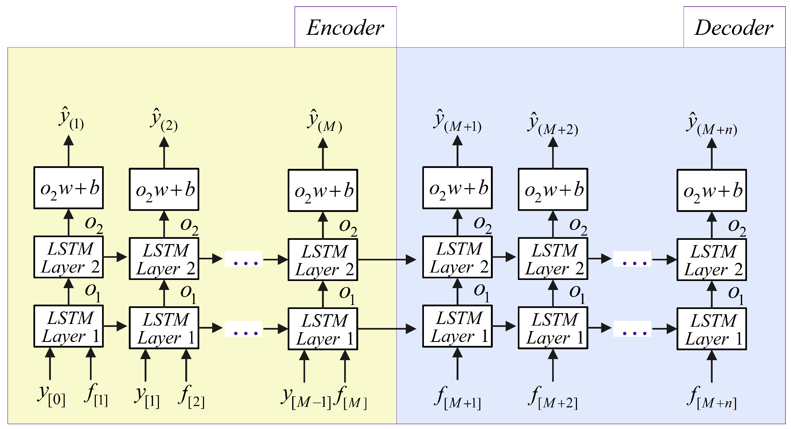
4.2. Lstm-Based Rnn for Electric Load Forecasting
A. Recurrent Neural Networks (RNNs)
B. LSTM-Based RNN Forecasting Scheme
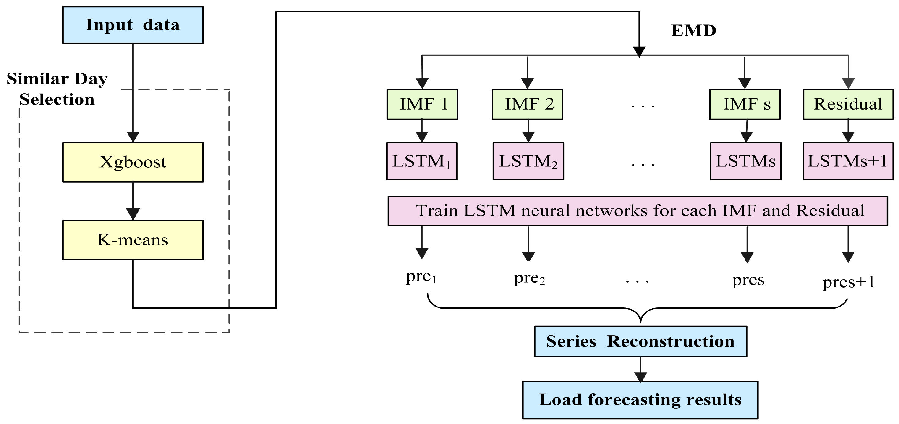
4.3. The Full Procedure of SD-EMD-LSTM Model
- Similar days selection. Calculate the features weight by xgboost method, then combined with K-means algorithm to determine the similar days cluster.
- Data decomposition. Take similar days load as input data, and decompose the input data into several intrinsic mode functions with EMD algorithm.
- Forecasting. Separated LSTM neural networks employed to forecast each IMF and residual, respectively. Reconstruct the forecasting values from each single LSTM model.
5. Numerical Experiments
5.1. Evaluation Indices for the Forecasting Performance
5.2. Empirical Results and Analysis
- (1)
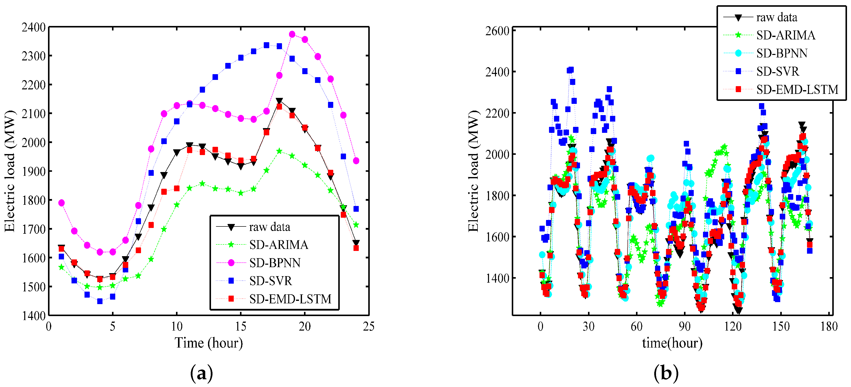
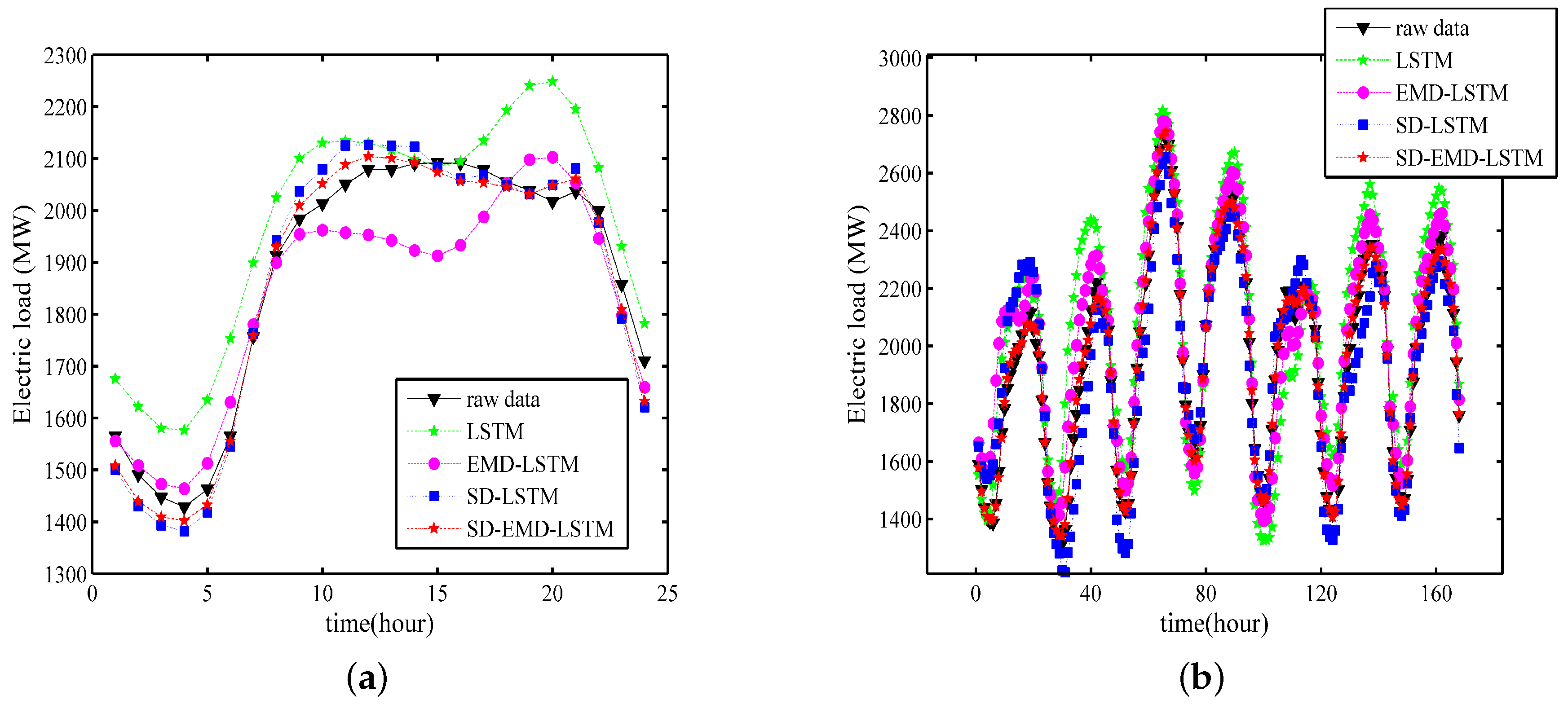
- The fitting effect of the hybrid model is evidently better than that of the single LSTM neural networks model in both time scales.
- (2)
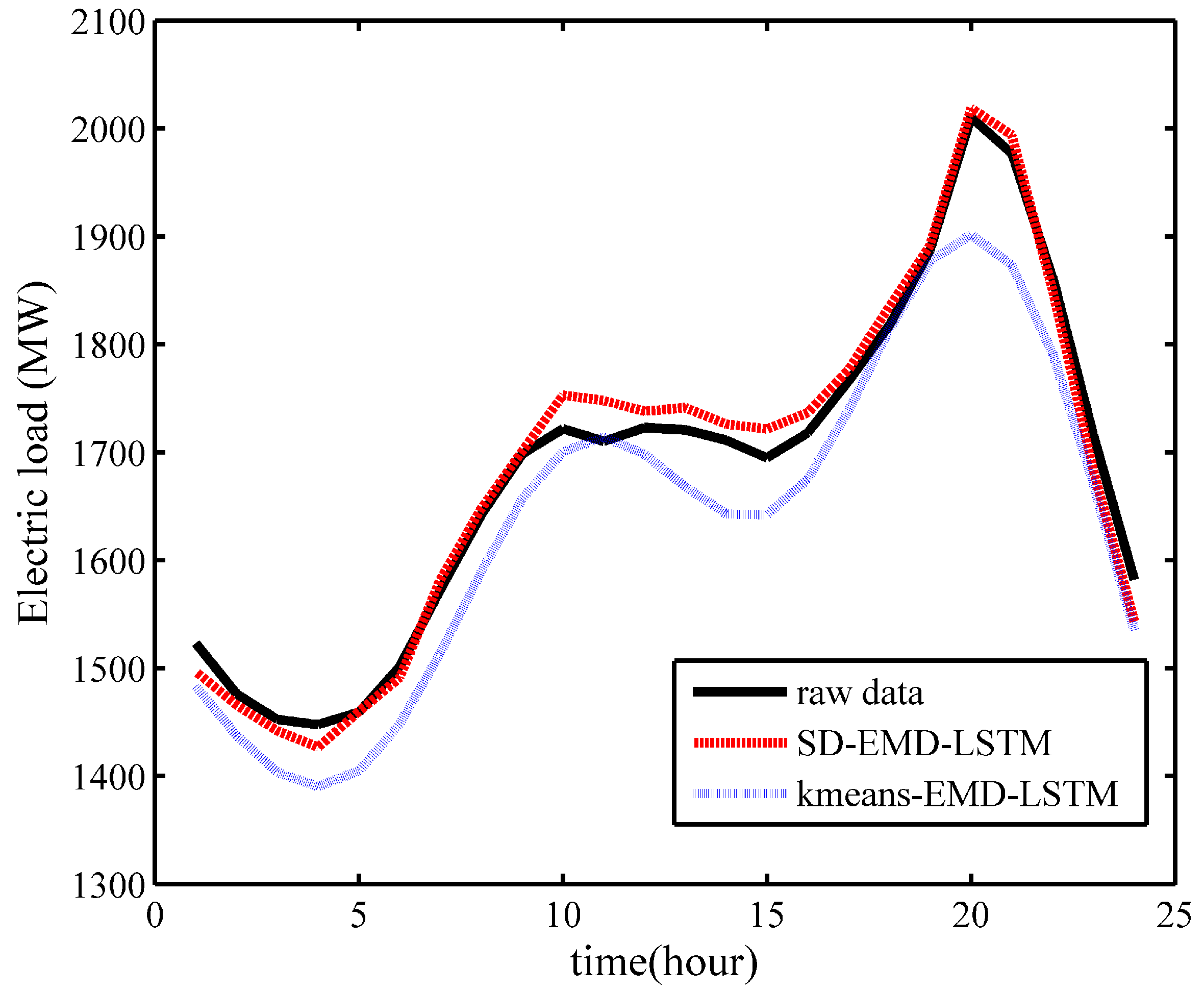
- The Xgboost-k-means method can effectively merge SDs into one cluster and prevent the LSTM neural networks from being trapped into a local optimum, thereby substantially improving the prediction accuracy.
- (3)
- The data decomposition method divides the singular values into separated IMFs and determines the general trend of the real time series, thereby effectively improving the performance and robustness of the model.
6. Conclusions
Acknowledgments
Author Contributions
Conflicts of Interest
References
- Dudek, G. Pattern-based local linear regression models for short-term load forecasting. Electr. Power Syst. Res. 2016, 130, 139–147. [Google Scholar] [CrossRef]
- Shenoy, S.; Gorinevsky, D.; Boyd, S. Non-parametric regression modeling for stochastic optimization of power grid load forecast. In Proceedings of the American Control Conference (ACC), Chicago, IL, USA, 1–3 July 2015; pp. 1010–1015. [Google Scholar]
- Christiaanse, W. Short-term load forecasting using general exponential smoothing. IEEE Trans. Power Appar. Syst. 1971, PAS-90, 900–911. [Google Scholar] [CrossRef]
- Kandil, M.; El-Debeiky, S.M.; Hasanien, N. Long-term load forecasting for fast developing utility using a knowledge-based expert system. IEEE Trans. Power Syst. 2002, 17, 491–496. [Google Scholar] [CrossRef]
- Sun, X.; Luh, P.B.; Cheung, K.W.; Guan, W.; Michel, L.D.; Venkata, S.; Miller, M.T. An efficient approach to short-term load forecasting at the distribution level. IEEE Trans. Power Syst. 2016, 31, 2526–2537. [Google Scholar] [CrossRef]
- Ghofrani, M.; Ghayekhloo, M.; Arabali, A.; Ghayekhloo, A. A hybrid short-term load forecasting with a new input selection framework. Energy 2015, 81, 777–786. [Google Scholar] [CrossRef]
- Mandal, P.; Senjyu, T.; Funabashi, T. Neural networks approach to forecast several hour ahead electricity prices and loads in deregulated market. Energy Convers. Manag. 2006, 47, 2128–2142. [Google Scholar] [CrossRef]
- Chen, Y.; Luh, P.B.; Guan, C.; Zhao, Y.; Michel, L.D.; Coolbeth, M.A.; Friedland, P.B.; Rourke, S.J. Short-term load forecasting: Similar day-based wavelet neural networks. IEEE Trans. Power Syst. 2010, 25, 322–330. [Google Scholar] [CrossRef]
- Mu, Q.; Wu, Y.; Pan, X.; Huang, L.; Li, X. Short-term load forecasting using improved similar days method. In Proceedings of the 2010 Asia-Pacific Power and Energy Engineering Conference (APPEEC), Chengdu, China, 28–31 March 2010; pp. 1–4. [Google Scholar]
- Arahal, M.R.; Cepeda, A.; Camacho, E.F. Input variable selection for forecasting models. IFAC Proc. Vol. 2002, 35, 463–468. [Google Scholar] [CrossRef]
- Raza, M.Q.; Khosravi, A. A review on artificial intelligence based load demand forecasting techniques for smart grid and buildings. Renew. Sustain. Energy Rev. 2015, 50, 1352–1372. [Google Scholar] [CrossRef]
- Velasco, L.C.P.; Villezas, C.R.; Palahang, P.N.C.; Dagaang, J.A.A. Next day electric load forecasting using artificial neural networks. In Proceedings of the 2015 International Conference on Humanoid, Nanotechnology, Information Technology, Communication and Control, Environment and Management (HNICEM), Cebu City, Philippines, 9–12 December 2015; pp. 1–6. [Google Scholar]
- Hernández, L.; Baladrón, C.; Aguiar, J.M.; Calavia, L.; Carro, B.; Sánchez-Esguevillas, A.; Pérez, F.; Fernández, Á.; Lloret, J. Artificial neural network for short-term load forecasting in distribution systems. Energies 2014, 7, 1576–1598. [Google Scholar] [CrossRef]
- Buitrago, J.; Asfour, S. Short-term forecasting of electric loads using nonlinear autoregressive artificial neural networks with exogenous vector inputs. Energies 2017, 10, 40. [Google Scholar] [CrossRef]
- Kaytez, F.; Taplamacioglu, M.C.; Cam, E.; Hardalac, F. Forecasting electricity consumption: A comparison of regression analysis, neural networks and least squares support vector machines. Int. J. Electr. Power Energy Syst. 2015, 67, 431–438. [Google Scholar] [CrossRef]
- Selakov, A.; Cvijetinović, D.; Milović, L.; Mellon, S.; Bekut, D. Hybrid pso-svm method for short-term load forecasting during periods with significant temperature variations in city of burbank. Appl. Soft Comput. 2014, 16, 80–88. [Google Scholar] [CrossRef]
- Niu, D.; Dai, S. A short-term load forecasting model with a modified particle swarm optimization algorithm and least squares support vector machine based on the denoising method of empirical mode decomposition and grey relational analysis. Energies 2017, 10, 408. [Google Scholar] [CrossRef]
- Liang, Y.; Niu, D.; Ye, M.; Hong, W.-C. Short-term load forecasting based on wavelet transform and least squares support vector machine optimized by improved cuckoo search. Energies 2016, 9, 827. [Google Scholar] [CrossRef]
- Kim, K.-H.; Park, J.-K.; Hwang, K.-J.; Kim, S.-H. Implementation of hybrid short-term load forecasting system using artificial neural networks and fuzzy expert systems. IEEE Trans. Power Syst. 1995, 10, 1534–1539. [Google Scholar]
- Suganthi, L.; Iniyan, S.; Samuel, A.A. Applications of fuzzy logic in renewable energy systems—A review. Renew. Sustain. Energy Rev. 2015, 48, 585–607. [Google Scholar] [CrossRef]
- Niu, D.-X.; Shi, H.-F.; Wu, D.D. Short-term load forecasting using bayesian neural networks learned by hybrid monte carlo algorithm. Appl. Soft Comput. 2012, 12, 1822–1827. [Google Scholar] [CrossRef]
- Sak, H.; Senior, A.; Beaufays, F. Long short-term memory recurrent neural network architectures for large scale acoustic modeling. In Proceedings of the Fifteenth Annual Conference of the International Speech Communication Association, Singapore, 14–18 September 2014. [Google Scholar]
- Gers, F.A.; Schmidhuber, J.; Cummins, F. Learning to forget: Continual prediction with lstm. Neural Comput. 2000, 12, 2451–2471. [Google Scholar] [CrossRef] [PubMed]
- Williams, R.J.; Zipser, D. A learning algorithm for continually running fully recurrent neural networks. Neural Comput. 1989, 1, 270–280. [Google Scholar] [CrossRef]
- Yang, Y.; Yu, D.J.; Cheng, J.S.; Shi, M.L.; Yu, Y. Roller bearing fault diagnosis method based on emd and neural network. J. Vib. Shock 2005, 1. [Google Scholar]
- Huang, N.E.; Shen, Z.; Long, S.R.; Wu, M.C.; Shih, H.H.; Zheng, Q.; Yen, N.-C.; Tung, C.C.; Liu, H.H. The empirical mode decomposition and the hilbert spectrum for nonlinear and non-stationary time series analysis. R. Soc. Lond. A Math. Phys. Eng. Sci. 1998, 454, 903–995. [Google Scholar] [CrossRef]
- Huang, B.; Kunoth, A. An optimization based empirical mode decomposition scheme. J. Comput. Appl. Math 2013, 240, 174–183. [Google Scholar] [CrossRef]
- An, X.; Jiang, D.; Zhao, M.; Liu, C. Short-term prediction of wind power using emd and chaotic theory. Commun. Nonlinear Sci. Numer. Simul. 2012, 17, 1036–1042. [Google Scholar] [CrossRef]
- Dong, Y.; Ma, X.; Ma, C.; Wang, J. Research and application of a hybrid forecasting model based on data decomposition for electrical load forecasting. Energies 2016, 9, 1050. [Google Scholar] [CrossRef]
- Mitchell, T.M. Machine Learning; McGraw Hill: Burr Ridge, IL, USA, 1997; Volume 45, pp. 230–247. [Google Scholar]
- Friedman, J.H. Stochastic gradient boosting. Comput. Stat. Data Anal. 2002, 38, 367–378. [Google Scholar] [CrossRef]
- Friedman, J.; Hastie, T.; Tibshirani, R. The Elements of Statistical Learning; Springer Series in Statistics; Springer: Berlin, Germany, 2001; Volume 1. [Google Scholar]
- Breiman, L.; Friedman, J.H.; Olshen, R.A.; Stone, C.J. Classification and Regression Trees; Wadsworth International Group, Chapman and Hall/CRC: Belmont, CA, USA, 1984. [Google Scholar]
- MacQueen, J. Some methods for classification and analysis of multivariate observations. In Proceedings of the Fifth Berkeley Symposium on Mathematical Statistics and Probability, Oakland, CA, USA, 21 June 1967; Volume 1, pp. 281–297. [Google Scholar]
- Hochreiter, S.; Schmidhuber, J. Long short-term memory. Neural Comput. 1997, 9, 1735–1780. [Google Scholar] [CrossRef] [PubMed]
- Witten, I.H.; Frank, E.; Hall, M.A.; Pal, C.J. Data Mining: Practical Machine Learning Tools and Techniques; Morgan Kaufmann: Burlington, MA, USA, 2016. [Google Scholar]
- Pascanu, R.; Mikolov, T.; Bengio, Y. On the difficulty of training recurrent neural networks. In Proceedings of the 30th International Conference on International Conference on Machine Learning, Atlanta, GA, USA, 16–21 June 2013; Volume 28, pp. 1310–1318. [Google Scholar]
- Bengio, Y.; Simard, P.; Frasconi, P. Learning long-term dependencies with gradient descent is difficult. IEEE Trans. Neural Netw. 1994, 5, 157–166. [Google Scholar] [CrossRef] [PubMed]
- Graves, A. Supervised sequence labelling. In Supervised Sequence Labelling with Recurrent Neural Networks; Springer: Berlin, Germany, 2012; pp. 5–13. [Google Scholar]


| Layers | Units | MAPE (Training) | MAPE (Testing) |
|---|---|---|---|
| 1 | 5 | 1.13 | 1.026 |
| 1 | 20 | 1.079 | 1.043 |
| 1 | 50 | 1.023 | 1.072 |
| 1 | 100 | 0.944 | 1.115 |
| 2 | 5 | 1.095 | 1.028 |
| 2 | 20 | 1.021 | 1.061 |
| 2 | 50 | 0.962 | 1.012 |
| 2 | 100 | 1.078 | 1.103 |
| 3 | 5 | 1.083 | 1.116 |
| 3 | 20 | 1.05 | 1.051 |
| 3 | 50 | 0.958 | 1.138 |
| 3 | 100 | 0.934 | 1.342 |
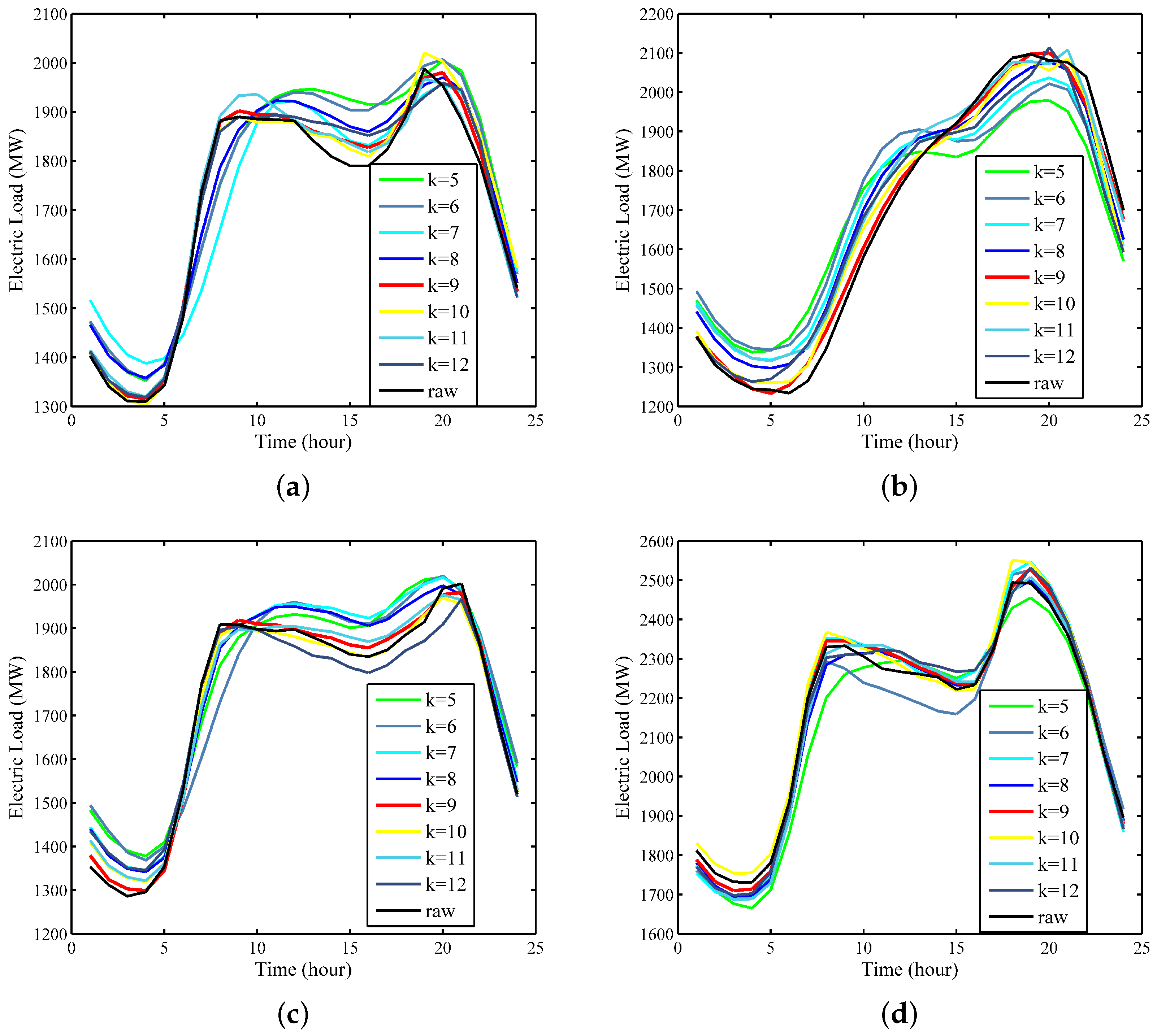
| k | 5 | 6 | 7 | 8 | 9 | 10 | 11 | 12 |
|---|---|---|---|---|---|---|---|---|
| MAPE(%) | 3.81 | 3.45 | 3.08 | 2.05 | 0.97 | 1.42 | 1.94 | 2.12 |
| Model | January | February | March | April | May | June | July | August | September | October | November | December |
|---|---|---|---|---|---|---|---|---|---|---|---|---|
| SD-EMD-LSTM | 1.03 | 0.96 | 0.83 | 1.09 | 0.77 | 0.93 | 0.96 | 0.88 | 1.06 | 1.12 | 0.91 | 1.12 |
| kmeans-EMD-LSTM | 2.11 | 2.17 | 1.98 | 2.56 | 1.83 | 2.16 | 1.96 | 2.03 | 2.08 | 1.79 | 2.04 | 2.18 |
| Hour | 1 | 2 | 3 | 4 | 5 | 6 | 7 | 8 | 9 | 10 | 11 | 12 |
| SD-EMD-LSTM | 1.77 | 1.42 | 1.73 | 2.00 | 1.87 | 1.63 | 0.81 | 0.20 | 1.09 | 1.99 | 1.75 | 0.96 |
| SD’-EMD-LSTM | 2.20 | 2.25 | 2.26 | 2.21 | 2.44 | 2.41 | 0.93 | 0.61 | 1.33 | 2.13 | 1.99 | 0.82 |
| 13 | 14 | 15 | 16 | 17 | 18 | 19 | 20 | 21 | 22 | 23 | 24 | Average |
| 0.49 | 1.57 | 1.22 | 0.47 | 0.27 | 0.71 | 0.29 | 0.46 | 0.25 | 1.33 | 1.48 | 0.52 | 1.10 |
| 0.12 | 1.01 | 1.46 | 1.05 | 1.41 | 2.40 | 2.32 | 1.07 | 0.15 | 1.73 | 1.02 | 0.33 | 1.44 |
| 24-h Ahead | 168-h Ahead | |||||||
|---|---|---|---|---|---|---|---|---|
| LSTM | SD-LSTM | EMD-LSTM | SD-EMD-LSTM | LSTM | SD-LSTM | EMD-LSTM | SD-EMD-LSTM | |
| January | 5.97 | 2.7 | 4.39 | 1.19 | 9.86 | 3.37 | 6.46 | 1.57 |
| February | 4.3 | 2.13 | 3.73 | 0.98 | 7.88 | 2.43 | 5.69 | 1.22 |
| March | 6.89 | 1.65 | 4.58 | 0.66 | 6.26 | 2.62 | 4.77 | 1.25 |
| April | 5.19 | 2.46 | 3.63 | 0.72 | 7.93 | 4.34 | 4.93 | 2.08 |
| May | 6.85 | 3.97 | 5.17 | 1.26 | 9.65 | 3.21 | 6.65 | 1.79 |
| June | 5.64 | 1.02 | 3.4 | 0.83 | 7.49 | 3.1 | 5.12 | 0.91 |
| July | 5.9 | 2.72 | 4.09 | 1.24 | 9.19 | 3.13 | 7.11 | 1.04 |
| August | 4.59 | 2.16 | 2.44 | 1.12 | 8.3 | 4.97 | 6.72 | 1.63 |
| September | 4.31 | 1.88 | 3.11 | 0.85 | 8.69 | 4.08 | 6.07 | 1.59 |
| October | 6.82 | 2.89 | 5.94 | 1.65 | 8.53 | 5.02 | 6.69 | 1.87 |
| November | 4.2 | 2.84 | 3.15 | 1.35 | 11.81 | 6.16 | 8.03 | 2.31 |
| December | 4.46 | 2.01 | 3.68 | 1.05 | 9.31 | 3.88 | 7.96 | 1.79 |
| Average | 5.43 | 2.37 | 3.94 | 1.08 | 8.74 | 3.86 | 6.35 | 1.59 |
| 24-h Ahead | 168-h Ahead | |||||||
|---|---|---|---|---|---|---|---|---|
| SD-ARIMA | SD-BPNN | SD-SVR | SD-EMD-LSTM | SD-ARIMA | SD-BPNN | SD-SVR | SD-EMD-LSTM | |
| January | 5.47 | 4.27 | 4.29 | 1.23 | 11.55 | 7.52 | 8.3 | 2.36 |
| February | 4 .43 | 1.79 | 1.96 | 0.75 | 6.97 | 9.03 | 2.29 | 1.05 |
| March | 3.34 | 2.84 | 3.5 | 1.12 | 5.04 | 3.42 | 5.25 | 1.29 |
| April | 4.05 | 3.74 | 6.08 | 1.04 | 7.94 | 4.56 | 7.52 | 1.09 |
| May | 7.88 | 4.43 | 2.43 | 0.95 | 9.36 | 5.26 | 2.41 | 1.83 |
| June | 5.49 | 5.68 | 2.93 | 0.82 | 6.44 | 9.26 | 6.96 | 1.92 |
| July | 3.61 | 1.92 | 2.07 | 1.12 | 8.5 | 3.81 | 3.18 | 1.69 |
| August | 5.86 | 2.68 | 3.58 | 1.87 | 10.65 | 9.12 | 6.29 | 2.03 |
| September | 4.51 | 1.86 | 3.68 | 0.98 | 9.72 | 2.19 | 4.33 | 1.26 |
| October | 6.07 | 4.28 | 6.51 | 0.76 | 7.98 | 5.77 | 8.85 | 1.28 |
| November | 8.51 | 3.85 | 2.13 | 0.99 | 6.11 | 4.52 | 3.72 | 1.75 |
| December | 10.05 | 5.71 | 3.47 | 0.87 | 11.73 | 5.44 | 9.5 | 1.22 |
| Average | 5.48 | 3.39 | 3.55 | 1.04 | 8.50 | 5.83 | 5.72 | 1.56 |
© 2017 by the authors. Licensee MDPI, Basel, Switzerland. This article is an open access article distributed under the terms and conditions of the Creative Commons Attribution (CC BY) license (http://creativecommons.org/licenses/by/4.0/).
Share and Cite
Zheng, H.; Yuan, J.; Chen, L. Short-Term Load Forecasting Using EMD-LSTM Neural Networks with a Xgboost Algorithm for Feature Importance Evaluation. Energies 2017, 10, 1168. https://doi.org/10.3390/en10081168
Zheng H, Yuan J, Chen L. Short-Term Load Forecasting Using EMD-LSTM Neural Networks with a Xgboost Algorithm for Feature Importance Evaluation. Energies. 2017; 10(8):1168. https://doi.org/10.3390/en10081168
Chicago/Turabian StyleZheng, Huiting, Jiabin Yuan, and Long Chen. 2017. "Short-Term Load Forecasting Using EMD-LSTM Neural Networks with a Xgboost Algorithm for Feature Importance Evaluation" Energies 10, no. 8: 1168. https://doi.org/10.3390/en10081168
APA StyleZheng, H., Yuan, J., & Chen, L. (2017). Short-Term Load Forecasting Using EMD-LSTM Neural Networks with a Xgboost Algorithm for Feature Importance Evaluation. Energies, 10(8), 1168. https://doi.org/10.3390/en10081168