Optimizing the Structure of Distribution Smart Grids with Renewable Generation against Abnormal Conditions: A Complex Networks Approach with Evolutionary Algorithms

Abstract

In this work, we describe an approach that allows for optimizing the structure of a smart grid (SG) with renewable energy (RE) generation against abnormal conditions (imbalances between generation and consumption, overloads or failures arising from the inherent SG complexity) by combining the complex network (CN) and evolutionary algorithm (EA) concepts. We propose a novel objective function (to be minimized) that combines cost elements, related to the number of electric cables, and several metrics that quantify properties that are beneficial for SGs (energy exchange at the local scale and high robustness and resilience). The optimized SG structure is obtained by applying an EA in which the chromosome that encodes each potential network (or individual) is the upper triangular matrix of its adjacency matrix. This allows for fully tailoring the crossover and mutation operators. We also propose a domain-specific initial population that includes both small-world and random networks, helping the EA converge quickly. The experimental work points out that the proposed method works well and generates the optimum, synthetic, small-world structure that leads to beneficial properties such as improving both the local energy exchange and the robustness. The optimum structure fulfills a balance between moderate cost and robustness against abnormal conditions. Our approach should be considered as an analysis, planning and decision-making tool to gain insight into smart grid structures so that the low level detailed design is carried out by using electrical engineering techniques.

1. Introduction

Motivation: The growing importance of renewable energy (RE) sources in the current energy mix is essential to decrease the economic and geopolitical dependence on fossil fuels and to reduce the emission of CO₂, one of the causes of climate change [1] and global warming [2]. Efficiently integrating distributed RE generation systems [3,4,5] is a key research topic because the most used renewable energies—photovoltaic (PV) solar energy [6,7], wind energy [8,9] and marine energy [10]—are intermittent and more difficult to store [11] and integrate without affecting the quality of the electrical network [12] or the electricity prices [13]. The current proliferation of small-scale urban PV in buildings [14] and urban wind generators [15] can help home electricity consumers become also producers (“prosumers”) [16] using the smart grid (SG) [17,18] and micro-grids ($\mu -$Gs) [19] concepts.

On the one hand, $\mu -$Gs exhibit the potential to cost-efficiently increase the use of RE along with the power supply reliability, as studied by Wang and Huang [20,21,22]. Specifically, [20] focuses on an optimization methodology that can efficiently integrate distributed energy resources by leveraging complementary resources, such as, solar and wind REs and energy storage. Using real data, [21] proposes a framework for planning micro-grid systems that aims at increasing the use of RE along with the reliability of power supply. Even more, the method proposed in [22] aims at enabling the bidirectional exchange of power among interconnected micro-grid, increasing the global efficiency. As long as the increasing penetration of distributed RE resources is one of the driving forces for micro-grids deployments [20,21,22], other catalysts for change are some new loads such as electric vehicles (EV) [23], data centers [24] and home RE-prosumers [25]. In this context, distribution systems (DSs) involve complex issues such as modeling their sensitivity with respect to distributed RE sources [26], the efficient control of distributed generation [4] or scheduling problems [27].

On the one hand, the SG paradigm is a relatively novel conception of the electric power network that, based on hi-tech monitoring, control and communication technologies [28,29,30], aims not only to efficiently integrate RE sources, but also to supply reliable and safe electric power. As mentioned, thanks to the efficient integration of distributed REs via the SG [31], electricity consumers can also become prosumers. The SG approach allows for the bidirectional exchange of electric energy at the local scale, which is very positive because it stimulates the local production (small-scale photovoltaic systems and small-wind turbines) and consumption, helping end-users obtain economic benefits by selling the energy generated in excess [30]. Integrating small-scale renewable energies is thus one of the driving forces that is fueling the evolution of conventional grids to smart grids. The second driving force, inter-related with the RE integration, is the pressure for unbundling the energy sector (as occurred in access telecommunication networks). Ideally, unbundling the electric sector would allow everyone to generate electricity, becoming a seller on a free energy market [30]. The distribution medium and low voltage parts of the power grid are the best candidates for unbundling the electric market. In this respect, smart grids are now becoming the enabling technology for not only the unbundling of electric sector through the integration of small-scale renewable energies, but also for the efficient integration of electric vehicles [23], which are increasingly important in the effort of reducing air pollution in big cities [1].

In this complex context, abnormal operating conditions in SGs with RE generation can be caused by the occurrence of: (1) random failures (such as imbalances between generation and consumption, the presence of overloads or failures arising from the inherent SG complexity [32], which can cause cascading failures); and (2) targeted or intentional attacks [28,29,33].

The vulnerability to abnormal operating conditions can be studied from different viewpoints that include methods from both the Electrical Engineering (EE) and the complex network (CN) fields. In turn, vulnerability in power grids using CN concepts is a broad research area that involves two different approaches [33]. The first one is based solely on “topological” concepts and use metrics such as the mean path length, the clustering coefficient or the betweenness centrality, among many others [33]. Aiming at enhancing the topological approach, the second “hybrid” methodology consists of introducing concepts arising from EE into the CN framework and takes advantage of novel electric metrics, such as those belonging to the “extended topological model” [34]. Regarding the first topological approach, there is a controversy [34,35] about whether or not it is able to give physical insights into all aspects of real power grids. The CN community argues that its approach does not aim to focus on the detailed operation, but to find out the unexpected emergence of collective behavior (for instance, the synchronization in smart grids [36]). Conversely, part of the EE community asserts that this leads to an unreasonable simplification [33,34,35]. This controversy, not yet resolved and recently discussed in [33], is the reason why we devote Section 5 to clarifying this and other issues, after introducing the necessary background.

Regardless of this debate, smart grids have been studied very recently by Pagani et al. [16,30,35,37,38], on the basis of real data extracted from low and medium voltage power grids. These works propose successful strategies to evolve the already deployed conventional grids into smart grids. Instead of grid evolution, the research line explored in [39,40,41] has adopted the different approach of generating synthetic smart grid structures.

Purpose and contributions: Within the aforementioned context, the two-fold purpose of this paper consists of: (1) modeling the topological structure of distribution SGs with RE generation using CN concepts; and (2) minimizing the negative effects of abnormal events by maximizing the grid robustness by using an evolutionary algorithm (EA) tailored for this goal. The SG is represented by a graph, a set of nodes (generators and loads) that are connected to each other by means of links (equivalently, electric cables). With this in mind, the contributions of our paper are:

• We model a smart grid with RE generators and loads (prosumers) as an undirected graph $\mathcal{G}$ so that each link allows for the bidirectional exchange of electric energy.
• We propose an objective function to be optimized that combines cost elements (related to the number and average length of links and also to the number of nodes with many links) and several properties that are beneficial for the SG (such as energy exchanges at local scale and high robustness and resilience). Our optimization problem includes some restrictions used in [30] and also others that help our EA find optimal synthetic structures for the SG, starting from scratch. This is a “greenfield” strategy, used by companies in those zones where they do not have infrastructure, deploying thus the new grid starting from scratch. This is another difference when compared to [30], in which the authors have just adopted a “brownfield” approach aiming at evolving the conventional low voltage power grid into a smart grid.
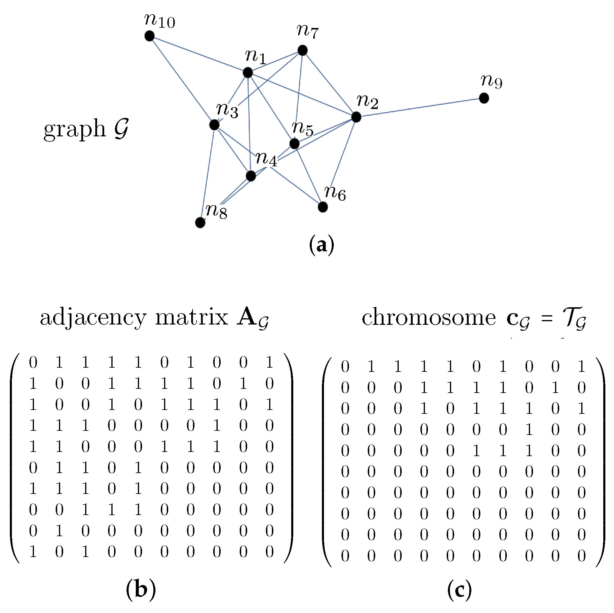
• We use an EA with a problem representation in which the chromosome ${\mathbf{c}}_{\mathcal{G}}$, which encodes each potential graph $\mathcal{G}$ (or individual), is the upper triangular matrix of its “adjacency matrix”, ${\mathbf{A}}_{\mathcal{G}}$. In this formulation, ${\mathbf{A}}_{\mathcal{G}}$ is a square, symmetric and binary matrix in which any element $a_{ij}$ encodes whether node i is linked to node j ($a_{ij}=1$) or not ($a_{ij}=0$) [42]. Since there is no self-connected node, the adjacency matrix has zeros on its main (principal) diagonal ($a_{ii}=0$). These are the reasons why the connection information in graph $\mathcal{G}$ is stored by its upper triangular matrix ${\mathcal{T}}_{\mathcal{G}}$. Thus, chromosome ${\mathbf{c}}_{\mathcal{G}}={\mathcal{T}}_{\mathcal{G}}$ encodes in a compact form the graph $\mathcal{G}$. As will be shown in detail in Section 2, this encoding is different from others found in the literature using EAs on graphs, such as, for instance, a chromosome formed by a one-dimensional array with N elements (the number of graph nodes) [43], N-length chromosome of two-dimensional elements [44] (where a node is specified by its location in the graph) or a set of vectors in which each allele (or gene value) represents a community [45]. The mutation and crossover operators are fully adapted to our encoding. This approach could be generalized by considering the strength of the connection between node i and j in terms of its link weight $w_{ij}$.

Paper Positioning: There are several research works that have applied EA and CN concepts to smart grids problems, which are partially related to our proposal and whose detailed discussion we postpone to Section 2 for clarity. There are also many research papers that focus on studying the smart grid from the point of view of CNs and graph theory and others that study graph problems using evolutionary computation (EC) techniques, in general, and EAs, in particular. However, a combined EA-CN approach to optimize the topology of smart grids, based on a variety of design constrains, has not yet been carried out to the best of our knowledge.

Practical perspectives: Our approach should be considered as a high level analysis, planning and decision-making tool to gain insights into how to design robust structures for smart grids and does not attempt and cannot replace the well-founded techniques of EE. Because of its importance and to make this paper stand by itself, we devote Section 5, as mentioned before, to justify the consistency of our proposal. The synthetic structure provided by our EA can be taken as a starting point to test whether or not it fulfills all of the electrical requirements. In this sense, our approach can be considered as a complementary high-level tool, so that the low level detailed design is carried out by using EE techniques.

Paper organization: The rest of this paper is organized as follows: Section 2 reviews those works that are related to our approach to a greater or lesser extent. Section 3 and Section 4 introduce, respectively, topological and hybrid CN concepts that will assist us in better explaining our method, while Section 5 discusses to what extent these CN approaches are useful in power grids. Section 6 and Section 7 state, respectively, the SG topology optimization problem and the particular EA we propose to solve it. Section 8 discusses the experimental work we have carried out. Finally, Section 9 summarizes the key findings and conclusions.

For the sake of clarity,

Table 1. List of symbols used in this work.

Symbol	Definition or Meaning
${\mathbf{A}}_{\mathcal{G}}$	Adjacency matrix of graph $\mathcal{G}$.
$a_{ij}$	Element of the adjacency matrix ${\mathbf{A}}_{\mathcal{G}}$ that encodes whether node i is linked to node j ($a_{ij}=1$) or not ($a_{ij}=0$).
$\overline{b_1}$	Mean value of betweenness $b_1$ or multi-scale vulnerability of order 1.
$\overline{b_2}$	Mean value of of the multi-scale vulnerability of order 2.
$b_l^p$	Betweenness centrality of link l.
$b_p\left(\mathcal{G}\right)$	Multi-scale vulnerability of order p of a graph $\mathcal{G}$. It is defined by Equation (9)
$\mathcal{C}=\overline{\mathcal{C}}$	Mean clustering coefficient of a network. It is defined by Equation (4).
$\mathbb{C}$	Set of all chromosomes.
$C_B\left(v\right)$	Betweenness centrality of node v. It quantifies how much a node v is found between the paths linking other pairs of nodes. It is defined by Equation (5).
${\mathbf{c}}_{\mathcal{G}}$	Chromosome that encodes the graph $\mathcal{G}$.
$C_i$	Clustering coefficient of node i. It is defined as the ratio between the number $M_i$ of links that exist between these $k_i$ vertices and the maximum possible number of links ($C_i\doteq 2M_i/k_i(k_i-1)$.
${\mathcal{C}}_{\mathrm{RG}}$	Clustering coefficient of a random graph
$\mathbf{D}$	Node degree matrix: $\mathrm{diag}(k_1,\cdots ,k_N)$. It is the diagonal matrix formed from the nodes degrees.
$d_E(n_i,n_j)$	Euclidean distance between any pair of nodes $n_i$ and $n_j$ in a spatial network.
$d_{ij}$	Distance between two nodes i and j. It is the length of the shortest path (geodesic path) between them, that is, the minimum number of links when going from one node to the other.
${\Delta }_{b_1}$	Coefficient of variation for betweenness. It is defined by Equation (10).
$f_{\mathrm{OBJ}}\left(\mathcal{G}\right)$	$=f_{\zeta }\left(\mathcal{G}\right)=$ objective function to be minimized. It is defined by Equation (11).
$\overline{f_{\zeta }}$	Mean value of the objective function $f_{\zeta }$.
$\mathcal{G}$	Graph representing a network.
$\mathbf{G}$	Set of all possible connected graphs $\mathcal{G}$ with N nodes and $M={\mathcal{N}}_l$ links.
$\mathbb{G}$	Set containing all of the candidate graphs.
${\mathcal{G}}_{\zeta }$	Optimum graph that solves the objective function with combination parameter $\zeta$.
$\langle k\rangle$	Average node degree: $〈k〉=\frac{1}{N}{\sum }_{i=1}^N{k}_i$.
$k_i$	Degree of a node i. It is the number of links connecting i to any other node. It is defined by Equation (2).
$k_{\mathrm{MAX}}$	Maximum node degree.
ℓ	Average path length of a network. It is the mean value of distances between any pair of nodes in the network. It is defined by Equation (3).
$\mathcal{L}$	Set of links (edges) of a graph.
${\mathbf{L}}_{\mathcal{G}}$	Laplacian matrix (or Kirchhoff matrix) of graph $\mathcal{G}$. It is defined by Equation (14).
${\ell }_{\mathrm{RG}}$	Average path length of a random graph.
${\lambda }_2\left(\mathcal{G}\right)$	Algebraic connectivity of graph $\mathcal{G}$.
M	Size of a graph $\mathcal{G}=(\mathcal{N},\mathcal{L})$. It is the number of links in the set $\mathcal{L}$. It is defined by Equation (1).
$\mathcal{N}$	Set of nodes (or vertices) of a graph.
N	Order of a graph $\mathcal{G}=(\mathcal{N},\mathcal{L})$. It is the number of nodes in set $\mathcal{N}$, that is the cardinality of set $\mathcal{N}$: $N=\left|\mathcal{N}\right|\equiv \mathrm{card}\left(\mathcal{N}\right)$.
$P\left(k\right)$	Probability density function giving the probability that a randomly selected node has k links.
$p_{\mathrm{cross}}$	Crossover probability.
$p_{\mathrm{mut}}$	Mutation probability.
$p_{\mathrm{selec}}$	Selection probability.
$p_{ij}$	Normalized weight of the link between nodes i and j: $p_{ij}\doteq \frac{w_{ij}}{{\sum }_j{w}_{ij}}.$
${\mathcal{P}}_{\mathrm{size}}$	Population size.
$\overline{\mathcal{S}}$	Average entropic degree.
${\mathcal{S}}_i$	Entropic degree of node i defined by Equation (6).
${\sigma }_{b_1}$	Standard deviation of betweenness.
${\mathcal{T}}_{\mathcal{G}}$	Upper triangular matrix of graph $\mathcal{G}$.
$T_{\mathrm{size}}$	Tournament size.
$\mathcal{W}$	Set of weight elements $w_{ij}$.
$w_{ij}$	Weight of link $l_{ij}$. It models the strength of the connection between node i and j.
$\zeta$	Parameter that controls the linear combination between components with opposing trends in the objective function to be minimized given by Equation (11).

lists the symbols used in this paper.

2. Related Work

For the sake of clarity, we have divided this section into two subsections. Section 2.1 discusses the research papers that focus on studying the smart grid from the viewpoint of complex networks and graph theory. Section 2.2 reviews those articles that tackle graph problems using evolutionary computation techniques, and EAs, in particular. To the best of our knowledge, there is no work combining both branches of knowledge for the problem of optimizing the structure of smart grids.

2.1. The Smart Grid as a Complex Network: Related Work

The SG paradigm has been modeled very recently as a complex network in a series of papers by Pagani et al. [16,30,35,46,47,48,49,50,51,52,53]. The approach adopted in these works is based on the need for improving the low voltage power grid, motivated in Section 1, and aims to analyze and adapt the already deployed distribution power grids on the basis of complex network approaches [30]. The ultimate goal of such a series of papers consists of putting into practice a decision support system to guide operators, utilities and policy makers to evolve the current grid to a more efficient smart grid.

These works cover a significant variety of research topics appearing in smart grids: the study of the potential of the SG to generate big data [48], the search for topological vulnerabilities [50], the study of the optimal spatial distribution [49], the use of agent-based systems for deregulated smart grids [52], the modeling of dynamic prices [51], the study of the last mile of the SG [47] and other technological aspects of SGs as CNs [16,30,46]. With regard to the latter, the authors carried out a topological analysis of some representative medium and low voltage power grids [46] and obtained a set of metrics based on topological properties in the effort of including their influence on the cost of electricity distribution. In the next step in this line of research, [16] has studied complex models to evaluate to what extent these allow for local electricity exchange, finding out that: (1) increasing the connectivity from the current value of the average degree $(\langle k\rangle \approx 2)$ to higher values is beneficial; and (2) the small-world complex network with average degree $\langle k\rangle \approx 4$ fulfills a feasible balance between performance enhancement and cost. The key, more recent work [30] explores a variety of feasible evolution strategies towards the SG and applies them to the real Dutch distribution system. An interesting finding in [30] is that increasing the connectivity leads to a topology that could lead to a more efficient and reliable electric grid.

While the aforementioned research line [16,30,35,46,47,48,49,50,51,52,53] proposes successful strategies to evolve the already deployed conventional grids into smart grids, the research line [39,40,41] has a different approach that consists of generating synthetic structures for smart grids. In these papers, the so-called “RT-nested-small world” model, based on analyses of real grid topologies and their electrical properties, has been proposed to create a large number of synthetic power grid test structures, with scalable size and the similar small-world topology and electrical features found in some real power grids [40].

As will be shown later on, our method has some aspects in common with both approaches. On the one hand, we state an optimization problem with some of the design constraints proposed in [30] (and with additional ones that we propose in this paper). On the other hand, our method generates synthetic structures, similar to the approach [39,40,41], but with the difference that we find the optimum synthetic structure by using an evolutionary algorithm.

2.2. Evolutionary Computation in Graph Approaches: Related Work

The use of evolutionary computation in the broad field of graphs has been carried out with different purposes and approaches. Aiming at discussing these within the goal of this paper, we use the encoding strategy adopted in each work as the comparative criterion. The reason is that the way candidate solutions are represented in EAs has a crucial influence on the design of evolutionary operators and on the algorithmic efficiency.

One of the most fertile areas of research combining graph theory and EC is focused on clustering in graphs. Cluster analysis is a key technique used for splitting a set of N objects into a number k of comparatively-homogeneous groups (clusters) based on their similarities [54]. The number of different attainable partitions in a clustering problem is given by the Stirling number of second kind, $S(N,k)$, and is known to be NP-hard when $k>3$ [54,55]. For instance, in a relative small graph with 50 nodes and five clusters, $S(50,5)\approx 7.4\times {10}^{32}$, which makes it convenient to use approximate methods such as those of evolutionary computation. In this respect, the approach in the recent work [43] consists of converting probabilistic datasets into probabilistic graphs with the purpose of clustering by using an EA. The genetic representation of this problem in this research work is a one-dimensional array having N elements, the number of graph nodes. This representation has been found to be feasible to extract neighborhood node information and uses such information to process probabilities on their links [43]. Graph partitioning via a multi-objective EA has been studied in [44] by encoding the problem with a chromosome that is a set of N (number of nodes) two-dimensional elements, in which any node is represented by its location in the graph. Instead of using EAs, the problem of optimal non-hierarchical clustering has been tackled in [54] by using a novel algorithm that combines differential evolution and k-means algorithms. Centered on social networks, the problem of community detection using graph-based information is tackled in [45] by applying graph clustering algorithms based on its topology information. Since any candidate solution should contain a group of communities, a chromosome encoding an individual in [45] is a set of vectors of binary values in which each allele represents a community composed by a set of binary values, one for each node in the social network. Partially related to the latter work, the paper [56] explores the feasibility of a spectrum optimization algorithm for community detection based on selecting those links to be removed by minimizing the algebraic connectivity metric. In the effort of making it applicable to large-scale networks, a greedy heuristic method has been tested to get the lower bound of optimal value. The problem of community detection, either disjoint or overlapping, has been tackled using a multi-objective EA [57] in which an individual consists of two components: the first one is a permutation of all nodes, while the second component is the set of communities. Another recent method that is gaining impulse is spectral clustering [58], which builds a similarity graph and applies spectral analysis to retain the data continuity in the cluster. The approach in [58] has proposed a novel algorithm inspired by the spectral clustering algorithm, the co-evolutionary multi-objective genetic graph-based clustering algorithm, which includes a variable number of clusters [58]. The encoding here is a simple label-based representation [58] inspired by the conventional integer encoding of genetic algorithms. Each individual is a q-dimensional vector (q being the number of data examples) with integer values between one and the number of clusters of the sub-population to which it is assigned. Very recently, reference [59] has explored a multi-objective EA for detecting overlapping communities. This differs from most other articles (focus on disjoint communities) in which each gene of the chromosome is an integer number that encodes the community label of the corresponding clique node of the maximal-clique graph. Also within the approach of maximum clique-finding problem, reference [60] explores an EA able to tackle the problems such as maximum independent set, set packing, set partitioning, set cover, minimum vertex cover, subgraph and double subgraph isomorphism. In the proposed approach, each problems is first mapped onto the maximum clique-finding problem, which is later tackled by an evolutionary strategy that represents each subgraph with a binary string.

Another important research field that combines CNs and EC consists of analyzing and/or generating CN structures [61,62,63]. On the one hand, reference [61] focuses on optimizing the structure of complex networks based on a memetic algorithm. Its problem encoding consists of an array containing the node number and the number of the node with which such a node is connected. On the other hand, the problem of automatically generating complex network models is tackling using genetic programming (GP) [62]. In this proposal, the goal is to find out those more appropriate network measures that capture as much as possible their structure, and the used tool is a GP that generates automatically CNs on which such measures can be tested. Similarly, the feasibility of a GP for the automatic inference of graph models for complex networks has also been explored in [63].

The graph coloring problem has also recently been tackled using an EA [64,65]. It aims at finding the minimum number of colors where each node dominates at least one non-empty color class and is an NP-complete for general graphs. In [65], the EA approach makes use of an encoding in which an individual is represented by a two-dimensional array with k columns, k being the number of colors used to color the nodes.

An interesting, partially related to our approach is the work carried out in [66], which focuses on a hybrid evolutionary graph-based multi-objective algorithm for the layout optimization of truss structures. The encoding of each candidate solution is composed of three matrices (the adjacency matrix of the simple graph model, the adjacency matrix corresponding to the weighted graph model and the coordinate matrix of nodes) along with two Boolean vectors (representing restricted nodes, which cannot be left out, and those movable ones, respectively). This approach is related to a certain degree with [67,68], which use a matrix representation based on the graph concept in truss topology optimization.

Finally, the main conclusion of the reviews carried out in Section 2.1 and Section 2.2 is that, to the best of our knowledge, there is no work combining complex network/graph theory and evolutionary algorithms in the effort to optimize the structure of smart grids starting from scratch, which is useful not only from a modeling and theoretical perspective, but also from the practical viewpoint as a high level tool for analysis, planning and decision-making.

3. Background: Complex Networks Concepts

The purpose of this section is to introduce basic definitions (Section 3.1) along with the concept of “small network” that, as will be shown, has important advantages for the network robustness (Section 3.2).

3.1. Some Useful Definitions in Complex Network

Any network can be mathematically represented by using a graph, $\mathcal{G}=(\mathcal{N},\mathcal{L})$, where $\mathcal{N}$ represents the set of nodes (or vertices) and $\mathcal{L}$ denotes the set of links (edges) [42]. The interested reader is referred to [42]; a very lucid and comprehensive description of complex networks, with many examples of their existence in a great variety of natural and artificial systems, can be found in [42]. The following list contains only those definitions that are important to understand our work [33,42,69,70]:

• An “undirected” graph is a graph for which the relationship between pairs of nodes are symmetric, so that each link has no directional character (unlike a “directed graph”). Unless otherwise stated, the term “graph” is assumed to refer to an undirected graph.
• A graph is “connected” if there is a path from any two different nodes of $\mathcal{G}$. A disconnected graph can be partitioned into at least two subsets of nodes so that there is no link connecting the two components (“connected subgraphs”) of the graph.
• A “simple graph” is an unweighted, undirected graph containing neither loops nor multiple edges.
• The “order” of a graph $\mathcal{G}=(\mathcal{N},\mathcal{L})$ is the number of nodes in set $\mathcal{N}$, that is the cardinality of set $\mathcal{N}$, which we represent as $\left|\mathcal{N}\right|$. We label the order of a graph as N, $N=\left|\mathcal{N}\right|\equiv \mathrm{card}\left(\mathcal{N}\right)$.
• The “size” of a graph $\mathcal{G}=(\mathcal{N},\mathcal{L})$ is the number of links in the set $\mathcal{L}$, $\left|\mathcal{L}\right|$, and can be defined (≐) as:

  $$M\doteq \sum _i\sum _j{a}_{ij}={\mathcal{N}}_l,$$

  (1)

  where $a_{ij}=1$ if node i is linked to node j and $a_{ij}=0$ otherwise. As mentioned before, $a_{ij}$ are the matrix elements of the adjacency matrix.
• The “degree” of a node i is the number of links connecting i to any other node and is simply:

  $$k_i\doteq \sum _j^N{a}_{ij}$$

  (2)
• The node degree is characterized by a probability density function $P\left(k\right)$ giving the probability that a randomly-selected node has k links.
• A “geodesic path” is the shortest path through the network from one nodes to another; or in other words, a geodesic path is the path that has the minimal number of links between two nodes. Note that there may be and often is more than one geodesic path between two nodes [42].
• The “distance” between two nodes i and j, $d_{ij}$, is the length of the shortest path (geodesic path) between them, that is the minimum number of links when going from one node to the other.
• The “average path length” of a network is the mean value of distances between any pair of nodes in the network [42]:

  $$\ell \doteq \frac{1}{N(N-1)}\sum _{i\ne j}{d}_{ij},$$

  (3)

  where $d_{ij}$ is the distance between node i and node j.
• The “clustering coefficient” is a local property capturing the density of triangles in a network. That is, two nodes that are connected to a third node are also directly connected to each other. Thus, a node i in a network has $k_i$ links that connects it to $k_i$ other nodes. The clustering coefficient of node i is defined as the ratio between the number $M_i$ of links that exist between these $k_i$ vertices and the maximum possible number of links ($C_i\doteq 2M_i/k_i(k_i-1)$. The clustering coefficient of the whole network is [33]:

  $$\mathcal{C}\doteq \frac{1}{N}\sum _i{C}_i,$$

  (4)

  that is, for a given node, we compute the number of neighboring nodes that are connected to each other and average this number over all of the nodes in the network.
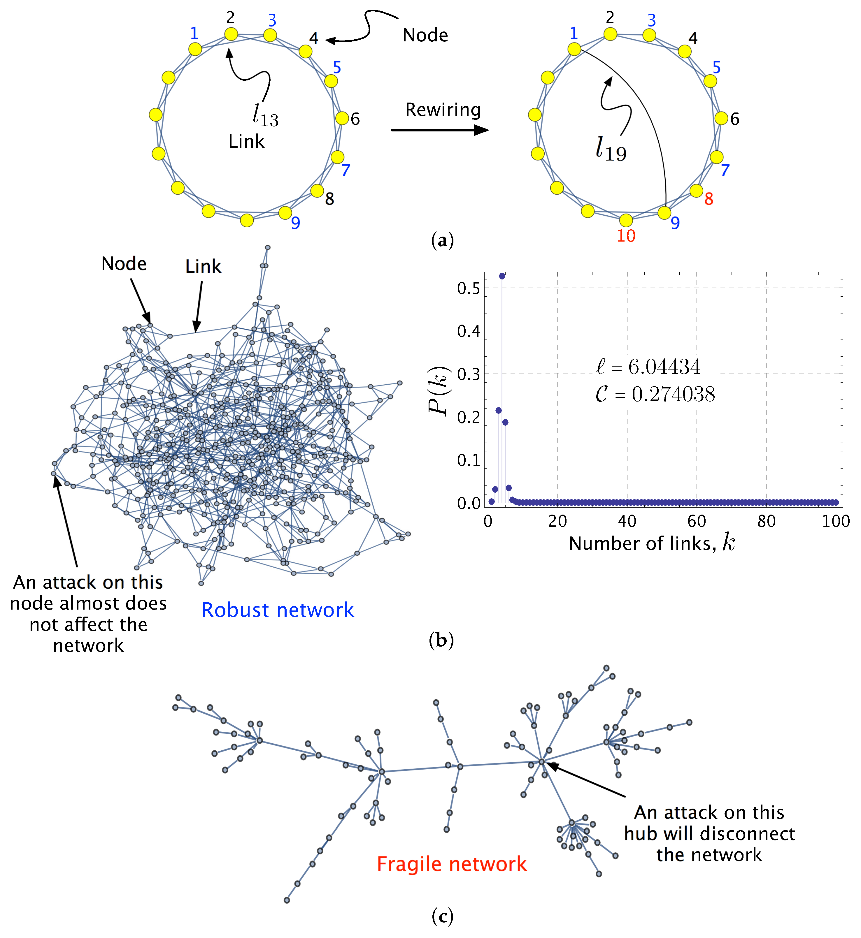
• The “betweenness centrality” quantifies how much a node v is found between the paths linking other pairs of nodes, that is,

  $$C_B\left(v\right)\equiv {\mathcal{B}}_v\doteq \sum _{s\ne v\ne t\in \mathcal{V}}\frac{{\sigma }_{st}\left(v\right)}{{\sigma }_{st}},$$

  (5)

  where ${\sigma }_{st}$ is the total number of shortest paths from node s to node t and ${\sigma }_{st}\left(v\right)$ is the number of those paths that pass through v. A high $C_B$ value for node v means that this node, for certain paths, is critical to support node connections. The attack or failure of v would lead to a number of node pairs either being disconnected or connected via longer paths.

3.2. Small-World Property and Its Importance in Robustness

There is a property of some complex networks that has been found to be especially beneficial for smart grids [16,30]: “small world”. Some properties of small-world networks that are interesting for the purpose of this paper are:

• A small-world network is a complex network in which the mean distance or average path length ℓ is small when compared to the total number of nodes N in the network: $\ell =\mathcal{O}(logN)$ as $N\to \infty$. That is, there is a relatively short path between any pair of nodes [71,72]. The term “small-world networks” is often used to refer Watts–Strogatz (WS) networks, first studied in [72]. It can be generated by the “rewiring” method shown in Figure 1a: Link $l_{13}$, which was connecting Node 1 to Node 3, is disconnected (from Node 3) and rewired to connect Node 1 to Node 9. In the resulting network, going from Node 1 to Node 9 only requires one jump via the rewired link (and thus, $d_{1,9}^{\mathrm{new}}=1$). However, in the original regular network, going from Node 1 to Node 9 through the geodesic or shortest path ($1\to 3\to 5$$\to 7\to 9$) involves four links ($d_{1,9}=4$). This leads to networks with small average shortest path lengths between nodes ℓ, and high clustering coefficient $\mathcal{C}$. Figure 1b shows the aspect and $P\left(k\right)$ of a WS we have generated with $N=100$ nodes and “rewiring probability” $p=0.2$. It has a short mean distance, $\ell \simeq 6.04$, and high clustering, $\mathcal{C}\approx 0.274$. Most of the small-world networks have exponential degree distributions [73].
• Figure 1b ($N=100$ and $p=0.2$) also illustrates that the architecture of real small-world networks is extremely heterogeneous: the vast majority of the elements are poorly connected, but simultaneously, few have a large number of connections [74]. The robustness of small-world network has been explored in [75,76] leading to the conclusion that, in a non-sparse WS network ($M\sim 2N$), simultaneously increasing both rewiring probability and average degree $(〈k〉=\frac{1}{N}{\sum }_{i=1}^N{k}_i)$ improves significantly the robustness of the small-world network.
• An interesting variation of the WS model is the one proposed by Newman and Watts [77] (NW small-world model) in which one does not break any connection between any two nearest neighbors, but instead, adds with probability p a connection between a pair of nodes. It has been found that for sufficiently small p and sufficiently large N, the NW model is basically equivalent to the WS model [78]. At present, these two models are together commonly termed small-world models.

Figure 1b also helps us introduce the concept of network robustness (or its inverse concept, vulnerability). It is related to the degree to which a network is able to withstand an unexpected event without degradation in its performance. It quantifies how much damage occurs as a consequence of such unexpected perturbation. Intuitively, the random failure of the marked link in Figure 1b does not affect the network functionality, while the targeted attack on the marked node in Figure 1c will make the network disintegrate in many unconnected parts before recovery. Figure 1b,c represent, respectively, a very robust network and another very fragile one. In particular, note in Figure 1c that, as most nodes have only a few connections and only a few nodes (“hubs”) have a high number of links, then the network is said to have no “scale” [79]. This is why they are called “scale-free” networks. A scale-free network can be generated by progressively adding nodes to an existing network by introducing links to nodes with “preferential attachment” [80,81] so that the probability of linking to a given node i is proportional to the number of existing links $k_i$ of the node. This is the so-called Barabási and Albert (BA) model.

As mentioned in Section 1, there are however some authors arguing that this topological approach should be enriched by adding electrical concepts. The following section introduces only those concepts that will assist us in explaining our proposal. For a more complete and in-depth discussion, which is beyond the scope of this paper, the interested reader is referred to [33,34].

4. Background: Hybrid Approaches Combining Complex Networks and Electric Engineering Concepts

As shown in detail in the review paper [33], there are some selected works [34,37] that emphasize that the topological approach may lead to inaccurate results because it does not capture some of the properties of power grids described by Kirchoff’s laws. Regarding this, there are some basic concepts that compel engineers to include electrical power engineering concepts [33]. The first one, in contrast to general purpose CNs, is that a power grid is a flow-based network in which electric power flowing between two nodes can involve many links. From the EE viewpoint, the topological distance metric in CN theory should be substituted by an “electrical distance”, involving line impedances [34]. The second cause is that, in conventional CN analysis, all elements are usually identical. This is not often the case in power transmission grids because of the existence of different types of nodes such as generation and load buses. Additionally, in power grids, transmission lines have flow limits. Based on these concepts, reference [34] argues that, when applying to power grids, the graph must be weighted (impedance, maximum power) and directed (since electric power flows from generators to loads). However, since smart grids are bidirectional; the corresponding graphs are undirected.

Thus, aiming at overcoming the mentioned limits of pure topological approaches, hybrid approaches combine CN and EE concepts [33]. An interesting research line belonging to hybrid approaches is the extended topological approach [34,82,83,84,85]. It includes in the CN methodology novel metrics such as the “entropy degree”. The entropic degree of a node i, denoted as ${\mathcal{S}}_i$, aims at including three elements in the topological definition of node degree when computed over a weighted network [82]: (1) the strength of the connection between node i and j in terms of link weight $w_{ij}$; (2) the number of links connected with such node; and (3) the distribution of weights among the links. The entropic degree of node i is defined as [82]:

$${\mathcal{S}}_i\doteq \left(1-\sum _j{p}_{ij}log{p}_{ij}\right)\sum _j{w}_{ij},$$

(6)

where $p_{ij}\doteq \frac{w_{ij}}{{\sum }_j{w}_{ij}}$ is the normalized weight of the link between nodes i and j.

The question arising here is whether or not applying CN approaches on the power grid is useful.

5. Discussion: Is the CN Approach Useful in Power Grids?

There are some selected papers [33,46,86,87,88,89,90] that point out that CN science is a unifying, powerful technique that enables one to analyze, within the same conceptual framework, a great variety of very different systems whose constituent elements are organized in a networked way. The CN community, including part of the electrical engineering community [91], argue that the CN approach does not aim to reflect the detailed operation of a given grid, but to discover the possible emergence of a systemic or collective behavior, beyond that of its single components. This is supported by a number of high-impact works [86,92,93,94,95,96,97]. An interesting example of its feasibility is the appearance of synchronization in smart grids [36]. However, the opposing community asserts that the pure topological CN approach loses the details of the physics behind Kirchhoff’s laws and fails at predicting important aspects of power grids. In this respect, as mentioned, hybrid approaches include concepts from EE [82,83,84,96,98,99,100,101,102]. Nonetheless, the CN approach with purely topological analysis (or even with extended ones to take into account minimal electrical information [34]) has been found to be useful to detect critical elements and to assess topological robustness [35,97,103]. Specifically, Luo and Rosas-Casals have recently reported studies [97,103] that aim at correlating electric-based vulnerability metrics (based on the extended topological approach) with real malfunction data corresponding to some European power transmission grids (Germany, Italy, France and Spain). The results, validated and proven by empirical reliability data, are statistically significant (Kolmogorov–Smirnov test) and suggest the existence of a relationship between structure (described by extended topological metrics) and dynamical empirical data.

Although much research must be carried out, the evidence in [97,103] opens a research line to find a more meaningful link between CN-based metrics and the real empirical data of power grids. The CN approach could be useful to make vulnerability assessment and to design specific actions to reduce topological fragility [34]. The analyses of [33,35,97,103] suggest that there is a connection between the topological structure and operation performance in a power grid because the structural change could disturb its operational condition and, as a consequence, degrade its operation performance. As a result, there is an increasing interest in analyzing structural vulnerability of power grids by means of the CN methodology. A deeper discussion on these issued can be found in [33] or in [35], where a lucid introduction to complexity science in the context of power grids is provided.

Regardless of which of the two confronting options is more accurate (or useful, depending on their purpose), there are some important practical issues related to whether or not there is a predominant power grid structure (and, in particular, whether there is an optimal topology for smart grids; Section 5.1) and whether or not it is better to model them with weighted graphs (Section 5.2).

5.1. Power Grids: Is There a Dominant Topology?

There are several graph structures aiming at abstracting the real power grid topology. For instance, the research in [72] points out that the U.S. western power grid seems to have a small-world network. However, the works by Cotilla-Sanchez et al. [104] and Hines et al. [100] show that (a) the explored power grid does not exhibit a small-world nature and that (b) a spatial approach to connectivity and distance fails in setting up a graph model representing the electrical properties of the grid. Furthermore, the research [80] suggested that the degree distribution of the power grid seemed to be scale-free following a power law distribution function, although not all of the subsequent works have agreed on this [33]. In this respect, some other works have also found that there are exponential cumulative degree functions, for instance in the Californian power grid [73] and in the whole U.S. power grid [105]. This notwithstanding, on the other hand, reference [106] has shown that the topologies of the North American eastern and western electric grids can be analyzed based on the Barabasi–Albert network model, with good agreement with the values of power system reliability indices previously obtained from standard power engineering methods. This suggests that scale-free network models are applicable to estimate aggregate electric grid reliability [34]. In addition to [72], there are also several works that report on power grids with small world nature: the Shanghai Power Grid (explored with a hybrid CN Direct Current (DC) and Alternating Current (AC) power flow models) [107], the Italian 380-kV, the French 400-kV and the Spanish 400-kV grids [108] or the Nordic power grid [109]. Rosas-Casals et al. [110], using data from thirty-three different European power grids, found that, although the different explored grids seem to have an exponential degree of distributions and most of them lack the small-world property, these grids showed however a behavior similar to scale-free networks when nodes are removed, concluding that this behavior is not unique to scale-free networks. This could suggest similar topological constraints, mostly associated with geographical restrictions and technological considerations [34]. Thus, the existence of several topologies in high-voltage transmission power grids suggest that there is no predominant structure, except for the fact that many grids have a heterogeneous nature [34] and that they are vulnerable to fails/attacks on the most connected nodes and robust against random failure.

However, in the particular case of smart grids, the small-world model seems to be beneficial. As pointed out in [16], the exchange of electric energy at the local scale could be very positive because it stimulates the local production and consumption of renewable-based electric energy (small-scale photovoltaic systems and small-wind turbines), helping the end-user obtain economic benefit by selling the energy produced in excess. Using real data from Dutch grids, and within the CN framework, the key contribution of [16] is to propose the use of CN theory (combined with global statistical measures) as a design tool to synthesize the best smart grid structures, in terms of performance and reliability (for a local energy exchange) and cabling cost. The authors in [16,30,35,46,47,48,49,50,51,52,53] made the conclusion that the small-world model seems to have many feasible features, not only structural, but also economic, related to electricity distribution.

Finally, and although not conclusive, power grids with a small network structure seem to be the most robust (except random networks) or, at least, seem to be those with the highest potential to improve robustness in a feasible way. In particular, the research work [75] has compared the robustness of random networks (ER), small-world (WS) and scale free (BA). Random networks are the most robust and scale-free the most vulnerable. Among the structures found in power grids (scale-free, small-world, as mentioned before), non-sparse small-world networks ($M\sim 2N$) are the most robust. According to [76], non-sparse small-world networks have also the beneficial property of increasing easily their robustness by a feasible method that consists of simultaneously increasing both the rewiring probability and the average degree $(〈k〉=\frac{1}{N}{\sum }_{i=1}^N{k}_i)$, which improves significantly the robustness of the small-world network.

5.2. Unweighted and Weighted Graphs: Which Is the Best?

An interesting point of discussion is whether the graph representing the particular grid under consideration uses either weighted or unweighted links. The review [33] points out that many works [46,86,89,90,105,106,108,109,110,111,112] have in common that each power grid has been represented using the simplest graph model: undirected and unweighted. This is because these approaches do not include any characterization of the link weights. Unweighted graphs are by far the most used representation in the group of references that tackle robustness in power grids from the pure topological CN viewpoint. On the contrary, most of the hybrid approaches, which include power flow models and/or electric-based metrics, made use of weighted graphs [33]. A deeper insight into the role of weighted links is given in [34], where it is noted that in power grids, transmission lines have power flow limits, which must be represented by weights $w_{ij}$ standing for the flow limit on line $l_{ij}\equiv l(i,j)$ linking nodes i and j. The authors in [34] argue that when applying CN analysis to power grids, the electrical power grid must be represented as a weighted and directed network graph $\mathcal{G}=(\mathcal{N},\mathcal{L},\mathcal{W})$, where $\mathcal{W}$ is the set of weight elements $w_{ij}$.

6. Proposal: Metrics, Objective Function and Problem Statement

6.1. Metrics to Construct the Objective Function

We have mentioned that in a smart grid made up of prosumer nodes, there should be a bidirectional interchange of energy at the local scale. Aiming at achieving this goal, the following features are beneficial:

• It is necessary for the SG to have a structure with reduces losses in the electric cables used to transport electric power from one node to another. This electrical restriction can be modeled using the condition:

  $$\ell ⩽logN,$$

  (7)

  which, as pointed out in [30], is related to giving a reduced path when moving from one node to another in a general purpose complex network. In the particular case of a smart grid, this may lead to a topology with limited losses in the circuits used to transfer electricity from one node to another. That is, it is a requirement related to the efficiency of the network. Along with the high clustering coefficient, this is also one of the properties of small-world networks, in which the mean distance or average path length ℓ is small when compared to the total number of nodes N in the network: $\ell =\mathcal{O}(logN)$ as $N\to \infty$. A small value of ℓ is also important from the economic viewpoint since it may lead to smaller cost.
• The entropic degree of a node i, ${\mathcal{S}}_i$, defined by Equation (6), has the advantage of providing a quantitative measurements of the importance of buses [82] in power grids by including the involved link weights and their number and distributions.
• Since the node degree $k_i$ of a node i is the number of links connecting i to any other node, its maximum value gets an upper limit related to the maximum power that a node can support:

  $$max\left(k_i\right)\le k_{\mathrm{MAX}}.$$

  (8)
  The value of $k_{\mathrm{MAX}}$ is related to the maximum power that a node is able to support and is directly related to its economic cost. In [30], average degree values $\langle k\rangle$ ranging from $\approx 3$ to $\approx 4$ lead to a good balance between performance and cost.
• The clustering coefficient defined by Equation (4) of a smart grid ${\mathcal{C}}_{\mathrm{SG}}$ should be higher than that of the corresponding random network (RN) with the same order (number of nodes) and size (number of links). This aims at assuring a local clustering among nodes because it is more likely that electricity exchanges occur in the neighborhood in a scenario with many small-scale distributed RE generators [30].
• We measure the network vulnerability by using the concept of multiscale vulnerability of order p of a graph $\mathcal{G}$ [113,114],

  $$b_p\left(\mathcal{G}\right)\doteq {\left(\frac{1}{{\mathcal{N}}_l}\sum _{l=1}^{{\mathcal{N}}_l}{b}_l^p\right)}^{1/p},$$

  (9)

  where $b_l^p$ is the betweenness centrality of link l. The multi-scale vulnerability $b_p$ of a graph $\mathcal{G}$ measures the distribution of shortest paths when links are failing (or attacked) [114] and is very useful when comparing the vulnerability of networks because it helps distinguish between non-identical although very similar network topologies [113]. As shown in [114], if we want to distinguish between two networks with graphs $\mathcal{G}$ and ${\mathcal{G}}^{*}$, one first computes $b_1$. If $b_1\left(\mathcal{G}\right)=b_1\left({\mathcal{G}}^{*}\right)$, then one takes $p>1$ and computes $b_p$ until $b_p\left(\mathcal{G}\right)\ne b_p\left({\mathcal{G}}^{*}\right)$. Using this approach, we have considered $b_2\left(\mathcal{G}\right)$. A network represented by a graph $\mathcal{G}$ is less vulnerable (more robust) than another ${\mathcal{G}}^{*}$ if $b_2\left(\mathcal{G}\right)<b_2\left({\mathcal{G}}^{*}\right)$. Please see [113,114] for further details.
• A coefficient of variation for betweenness [30],

  $${\Delta }_{b_1}=\frac{{\sigma }_{b_1}}{\overline{b_1}},$$

  (10)

  where ${\sigma }_{b_1}$ is the standard deviation of betweenness ($b_1$) and $\overline{b_1}$ is the mean value of betweenness. Distributions with ${\Delta }_{b_1}<1$ are known as low-variance ones. This requirement leads to network resilience by providing distributions of shortest paths that are more uniform among all nodes. See [30] for further details.

6.2. Proposed Objective Function

We propose an objective function (to be minimized), which is a combination of different functions related to topological and hybrid CN metrics mentioned before in Lists 1–6 in Section 6.1. The objective function is:

$$f_{\mathrm{OBJ}}\left(\mathcal{G}\right)=f_{\zeta }\left(\mathcal{G}\right)=\zeta ·({\mathcal{N}}_l+\ell +\frac{1}{\overline{\mathcal{C}}})+(1-\zeta )·(b_2+\frac{{\sigma }_{b_2}}{\overline{b_2}}),$$

(11)

where ${\mathcal{N}}_l$ is the number of links, ℓ is the average path length, $\overline{\mathcal{C}}$ is the mean clustering coefficient and $b_2$ is the multi-scale vulnerability of order 2. The rest of the components have already been defined before. Note that $f_{\mathrm{OBJ}}$ is only one of the possible functions among several ones that aim at:

• Reducing ${\mathcal{N}}_l$ in the effort of decreasing the economic cost and the electric losses in the links used to transport electricity from one node to another. Reducing ${\mathcal{N}}_l$ makes the network less robust. This is because the minimum value of $b_2$, $b_{2,\min }=1$ [113], is reached for the “fully-connected network” or “completely-connected graph” in which any node is connected with all of the others. As the number of links decreases, the network becomes increasingly fragile and $b_2>1$. Reducing ${\mathcal{N}}_l$ to a great extent leads to an inexpensive, but very fragile structure ($b_2\gg 1$ [113,114]). Thus, the decrease of the number of links and the increase of the robustness have opposite tendencies. This is why we propose a balance between ${\mathcal{N}}_l$ and $b_2$ via the weight parameter $\zeta$, which controls the linear combination between constituents with opposing trends.
• Reducing $b_2$ (approaching one from above) to increase robustness and also $\frac{{\sigma }_{b_2}}{\overline{b_2}}$ to improve resilience.
• Reducing ℓ along with maximizing $\overline{\mathcal{C}}$ leads to a small-world structure.
• Increasing $\overline{\mathcal{C}}$ aiming to stimulate the local electricity exchanges in scenarios with many small-scale distributed RE generators.

6.3. Problem Statement

Let N be the “order” or the number of nodes (generators, loads) of the graph representing a smart grid. The number of links ($M={\mathcal{N}}_l=$ network size) to connect the N nodes and the specific way in which these nodes connect to each other are two of the aspects to be determined. Let $\mathbf{G}$ be the set of all possible connected graphs $\mathcal{G}$ with N nodes and $M={\mathcal{N}}_l$ links. A graph is connected if there is at least a path between every pair of nodes.

The problem consists of finding the topological structure (the network, or equivalently, the optimum graph $\widehat{\mathcal{G}}$) that minimizes the objective function $f_{\mathrm{OBJ}}$ stated by Equation (11),

$$\widehat{\mathcal{G}}=arg\underset{\mathcal{G}\in \mathbf{G}}{min}{f}_{\mathrm{OBJ}}\left(\mathcal{G}\right),$$

(12)

subject to a the condition that the graph $\mathcal{G}$ must be connected,

$${\lambda }_2\left(\mathcal{G}\right)>0.$$

(13)

Parameter ${\lambda }_2$ is called “algebraic connectivity” (or the Fiedler eigenvalue) [113] and, in graph theory, is one of the available parameters that can be used to mathematically measure to what extent a graph is connected. The algebraic connectivity ${\lambda }_2$ is a positive real number whose magnitude quantifies the level of connectivity in the graph. Larger values of algebraic connectivity represent higher robustness against efforts to break the graph into isolated parts. In the opposite limit, ${\lambda }_2=0$ means that the network has been broken into several disconnected parts. The algebraic connectivity ${\lambda }_2$ is computed as the second smallest eigenvalue of the “Laplacian matrix” of a graph $\mathcal{G}$, ${\mathbf{L}}_{\mathcal{G}}$. The Laplacian matrix, sometimes also called the admittance matrix or Kirchhoff matrix, is an $N\times N$ symmetric matrix defined by: [113]

$${\mathbf{L}}_{\mathcal{G}}={\mathbf{D}}_{\mathcal{G}}-{\mathbf{A}}_{\mathcal{G}},$$

(14)

where ${\mathbf{D}}_{\mathcal{G}}=\mathrm{diag}(k_1,\cdots ,k_N)$ is the node degree matrix, which is the diagonal matrix formed from the nodes degrees, and ${\mathbf{A}}_{\mathcal{G}}$ is the adjacency matrix of graph $\mathcal{G}$.

7. Proposed Evolutionary Algorithm

7.1. Basic Concepts

An EA is an optimization, population-based algorithm, inspired by the principles of natural selection and genetics, which is able to tackle complex problems [115,116] such as the one formulated. Among these advantages, EAs do not require derivative information and are able to optimize functions with a large number of continuous or discrete variables, finding the global solution for multi-local extrema problems [117]. As discussed in Section 2.2, although GA and EA are sometimes used interchangeably in the reviewed works, in this paper, we prefer to use the term EA since, as will be explained in Section 7.2.1; we have encoded each feasible solution as a binary triangular matrix, instead of a bit-string. For further details about this, the interested reader is referred to [118].

The underlying concepts of EAs and the way they are computationally implemented are inspired by the way Nature finds out solutions to extremely complex problems, such as the “survival of the fittest” individual in a evolving ecosystem [115,117]. Aiming at better explaining our approach, it is convenient to introduce here two biological phenomena from which EAs are inspired: (1) the external characteristics (“phenotype”) of living beings are encoded (represented) using genetic material (“genotype”); and (2) evolution is the result of the interaction between the random creation of new genetic information and the selection of those living beings that are best adapted to the environment [117].

7.1.1. Genotype-Phenotype Relationship

As mention, in natural evolution, genotype is the genetic information that encodes and causes the phenotype (all external characteristics) of a living being (or “individual”). Specifically, each characteristic is encoded by a “gene”, a “chromosome” being the set of these genes [117]. Each gene is located at a particular position on the chromosome and can exhibit different values (“allele”).

7.1.2. Natural Evolution

The random creation of new genetic information in Nature may lead to a better (or sometimes, worse) ability to survive. The better a living being is adapted to its environment, the higher its probability of survival is. This is called “survival of the fittest”. In turn, the longer the individual’s life is, the higher its probability of having descendants. In the procreation process, the parent chromosomes are crossed or combined (“recombination”) to generate a new chromosome (which encodes the offspring). With very small probability, “mutations” (or random variations in genes) can occasionally occur, caused by external factors (for instance, radiation) or simply by unavoidable errors when copying genetic information. This leads to offspring with new external properties, which are different from those of their predecessors. If such arising external characteristic makes the offspring better adapted to the environment, its probability of survival and having descendants increases. In turn, part of the offspring can inherit the mutated genes (and thus the corresponding external characteristic), which can be passed from generation to generation. These natural processes make the population evolve, resulting in the emergence of individuals better adapted to the environment and in the extinction of those less fitted. For deeper details about the main similarities and differences between natural evolution and evolutionary algorithms, the interested reader is referred to [115].

7.2. Evolutionary Algorithm Used

The analogy of our problem with the biological metaphor described is that we are looking for the “best graph” $\widehat{\mathcal{G}}$ that minimizes the objective function $f_{\mathrm{OBJ}}$ in Equation (12). In this search, a very large number of possible graphs $\mathcal{G}$ has to be evaluated aiming at computing the corresponding value $f_{\mathrm{OBJ}}\left(\mathcal{G}\right)$. Each possible graph is a candidate, trial solution or “individual”. The complete set of individuals is called the “population”. The extent to which a candidate solution is able to solve our problem is the “fitness of the individual”. The smaller the $f_{\mathrm{OBJ}}$ value of an individual, the better the fitness of the individual.

Just like in natural evolution, each individual or candidate solution is encoded using a chromosome, a kind of representation that eases the problem solution because it transforms the real search space into another in which working is much easier. The population is evolved via the application of genetic operators that mimic the natural processes of reproduction, mutation and selection.

7.2.1. Encoding Method

In our problem, the chromosome ${\mathbf{c}}_{\mathcal{G}}$, which encodes each potential graph $\mathcal{G}$ (or individual), is the upper triangular matrix of its adjacency matrix ${\mathbf{A}}_{\mathcal{G}}$. In this formulation, ${\mathbf{A}}_{\mathcal{G}}$ is a square, symmetric and binary matrix whose elements encode whether a node is linked ($a_{ij}=1$) to another adjacent one in the graph or not ($a_{ij}=0$). Since there is no node self-connected, the adjacency matrix has zeros on its main (principal) diagonal (($a_{ii}=0$)). These are the reasons why all of the information of link connections of graph $\mathcal{G}$ is stored by the upper triangular matrix ${\mathcal{T}}_{\mathcal{G}}$. Thus, chromosome ${\mathbf{c}}_{\mathcal{G}}={\mathcal{T}}_{\mathcal{G}}$ encodes in a compact form the information of the adjacency matrix ${\mathbf{A}}_{\mathcal{G}}$ of graph $\mathcal{G}$ (or individual).

For illustrative purposes, Figure 2a shows a simple random graph with 10 nodes and 20 links, while Figure 2b,c represents its corresponding adjacency matrix (${\mathbf{A}}_{\mathcal{G}}$) and its upper triangular matrix (${\mathcal{T}}_{\mathcal{G}}$ or chromosome ${\mathbf{c}}_{\mathcal{G}}={\mathcal{T}}_{\mathcal{G}}$ encoding the information of individual $\mathcal{G}$), respectively.

In the discussions that follow, the terms “individual” and “chromosome” are used interchangeably because each chromosome uniquely represents each solution in the actual search space. This strategy can be considered as transforming the actual search space into another in which the computational working is much easier. From a mathematical point of view, if $\mathbb{G}$ is the set containing all of the candidate graphs and $\mathbb{C}$ is the set of chromosomes that encodes each of them (${\mathbf{c}}_{\mathcal{G}}$), this representation is equivalent to defining a bijection,

$$\Xi :\mathbb{G}⟷\mathbb{C}$$

(15)

so that any candidate graph is represented by a unique chromosome $\Xi \left({\mathbf{A}}_{\mathcal{G}}\right)={\mathbf{c}}_{\mathcal{G}}={\mathcal{T}}_{\mathcal{G}}$.

7.2.2. Initial Population

The size of the initial population (number of chromosomes), ${\mathcal{P}}_{\mathrm{size}}$, is a crucial parameter for EA performance [118]. On the one hand, a large population could cause more diversity of candidate solutions (and thus, a higher search space), leading to a slower convergence. On the other hand, too small a population leads to reduced diversity: only a limited part of the search space will be explored. This increases the risk of prematurely converging to a local extreme. In our specific problem, after a number of experiments, the initial population has been chosen as ${\mathcal{P}}_{\mathrm{size}}=50$ individuals, as a tradeoff between computational complexity and performance.

As important as the population size is the way in which such an initial population is generated. Usually, the initial population is initialized at random. This strategy is appropriate for those problems in which there is no information about how the solution will be. However, there are problems in which a non-random, domain-specific initial population is more suitable [119]. This is the case of our problem since we have information about a suitable (although non-optimum) solution: small-world networks have been found to exhibit beneficial properties in some smart power grids. See [30] for a more detailed explanation. In our preliminary work, we have found that the EA works better if the initial population is generated as follows:

• Fifty percent of ${\mathcal{P}}_{\mathrm{size}}$ are Watts–Strogatz random graphs (with small-world properties, including short average path lengths and high clustering) with rewiring probability ranging from ${10}^{-2}$ to one.
• Fifty percent of ${\mathcal{P}}_{\mathrm{size}}$ are Erdős–Rényi (ER) random graphs with N nodes and $N\times 5$ links.

Figure 3 shows some examples of four graphs belonging to the initial population.

An important point is to ensure that any graph $\mathcal{G}$ in the initial population is connected by checking that it fulfills the condition ${\lambda }_2\left(\mathcal{G}\right)>0$ [113].

This approach to generate an SG domain-specific aims to reduce the number of searches within the solution space and to assist operators in finding the global minimum quickly.

7.2.3. Implementation of Evolutionary Operators

Selection Operator

Selection operators can be basically classified into two classes [118]: fitness proportionate selection (such as roulette-wheel selection and stochastic universal selection) and ordinal selection (tournament selection and truncation selection) [118]. After a number of experiments, we have selected as the selection operator the tournament selection. This strategy is one of the most widely-used selection operators in EAs since it performs well in a broad variety of problems, is susceptible to parallelization and can be implemented efficiently [118,120]. A very clear description of its key concepts and further details can be found in [120].

Tournament selection basically aims at selecting individuals based on the direct comparison among their fitness. In our problem, a candidate solution, a graph $\mathcal{G}$, encoded by chromosome ${\mathbf{c}}_{\mathcal{G}}$ is more fit than another, ${\mathbf{c}}_{\mathcal{H}}$, if the corresponding objective function $f_{\mathrm{OBJ}}$ is better (lower):

$$f_{\mathrm{OBJ}}\left({\mathbf{c}}_{\mathcal{G}}\right)<f_{\mathrm{OBJ}}\left({\mathbf{c}}_{\mathcal{H}}\right).$$

(16)

The simplest tournament selection operator consists of picking out at random two individuals (contenders) from the population and carrying out a combat (tournament) to elucidate which one will be selected. In particular, each combat involves the generation of a random real number $n_{\mathrm{tour}}\in [0,1]\subset \mathbb{R}$ to be compared to a prearranged selection probability, $p_{\mathrm{selec}}$. If $n_{\mathrm{tour}}\le p_{\mathrm{selec}}$, then the stronger (fitter or best) candidate is selected, otherwise the weaker candidate is selected. The probability parameter $p_{\mathrm{selec}}$ gives a suitable strategy for adjusting the selection pressure. To favor best (fittest) candidates, $p_{\mathrm{selec}}$ is usually set to be $p_{\mathrm{selec}}>0.5$ [120].

This simplest implementation of tournament with only two competitors (tournament size $=2$) can be generalized to involve more than two individuals. As shown in [120], the selection pressure can be adjusted by changing the tournament size. If the tournament size increases, weak individuals have a smaller probably of being selected. That is, the more competitors, the higher the resulting selection pressure.

Regarding this, the tournament selection operator we have implemented has a tournament size of $T_{\mathrm{size}}={\mathcal{P}}_{\mathrm{size}}$$=50$ contenders (that is, all individuals are fighting each other) and a selection probability, $p_{\mathrm{selec}}=0.8$. As mentioned, $p_{\mathrm{selec}}>0.5$ favor best (fittest) candidates [120]. The individual that accumulates the most wins is selected as the one that pass to the next generation in the selection process.

Crossover Operator

The crossover operator works as follows:

• Select at random ($p_{\mathrm{cross}}$) two individuals from the population (father and mother).
• Select at random the same row in the parents.
• Exchange the selected rows between the father and the mother, which leads to two child chromosomes.

Mutation Operator

Mutation operators are designed to generate diversity in each generation and aim at exploring the whole search space by introducing local changes with very small probability. Specifically, the implemented mutation operator selects at random an individual with a given probability $p_{\mathrm{mut}}$. The mutation operator then picks out at a random row (of the upper triangular matrix representing such an individual). Note that row “i” encodes how node i is connected to others: element $a_{ij}=1$ means that there is a link between nodes i and j. The next step that the operator makes is to select at random two elements of the row and to perform a permutation. This is equivalent to rewiring the links of node i to other nodes and ensuring that: (1) node i is not disconnected from the rest of the network and (2) that the degree of node i remains unchanged, despite having made the mentioned rewiring.

8. Experimental Work

8.1. Methodology

The EA is stochastic as it begins with a population randomly generated (see Section 7.2.2), and then evolutionary probabilistic operators are applied to the population in each generation. The result gets better ($f_{\mathrm{OBJ}}$ is reduced) quickly with the first iterations (generations) until it ends up stagnating, converging to a near-optimal result. As the EA is stochastic, obtaining statistical values is compulsory. This is the reason why the EA has been repeated 20 times, which have been found long enough.

The values for the EA parameters that we have considered in the experimental work described below are: $T_{\mathrm{size}}={\mathcal{P}}_{\mathrm{size}}$$=50$ graphs (50% being WS small-world graphs, with rewiring probability ranging from ${10}^{-2}$ to 1, and 50% being ER random graph with N nodes and $N\times 5$ links), $p_{\mathrm{selec}}=0.8$, $p_{\mathrm{mut}}=0.09$ and $p_{\mathrm{cross}}=0.2$.

For illustrative purposes, Figure 4 shows the mean value (a) and variance (b) of $f_{\mathrm{OBJ}}=f_{0.7}$ as a function of the number of generations.

8.2. Results: Optimizing the Structure

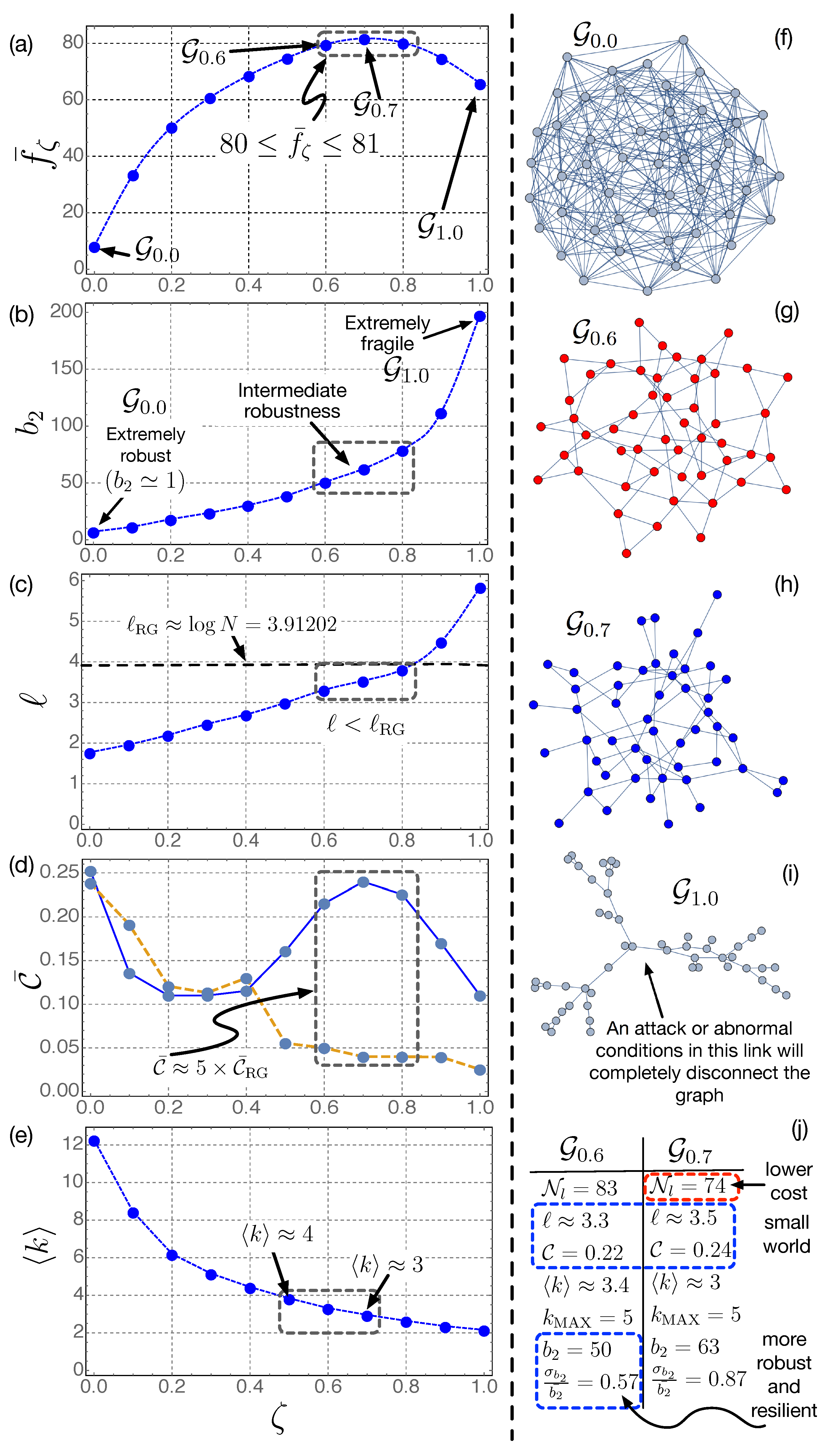
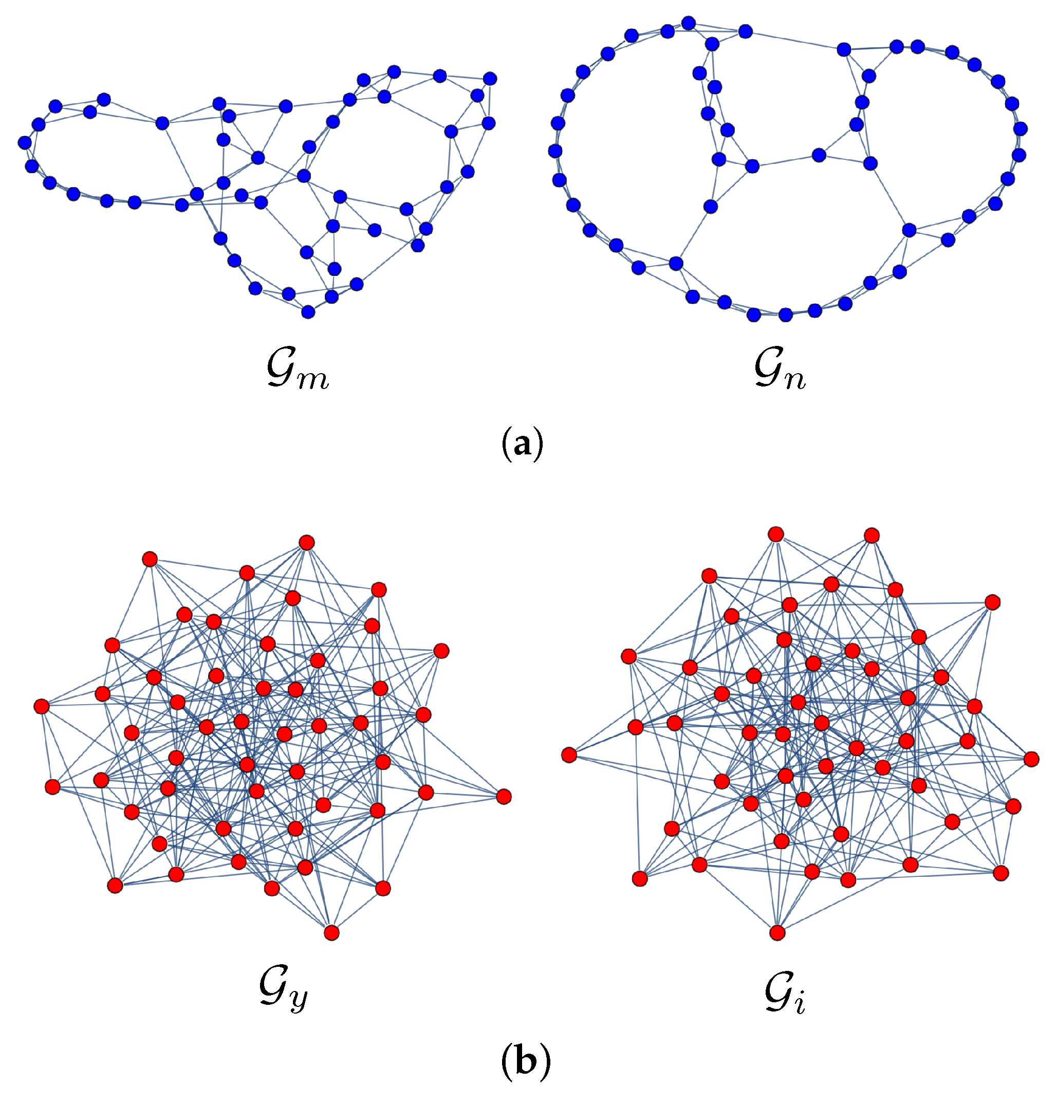
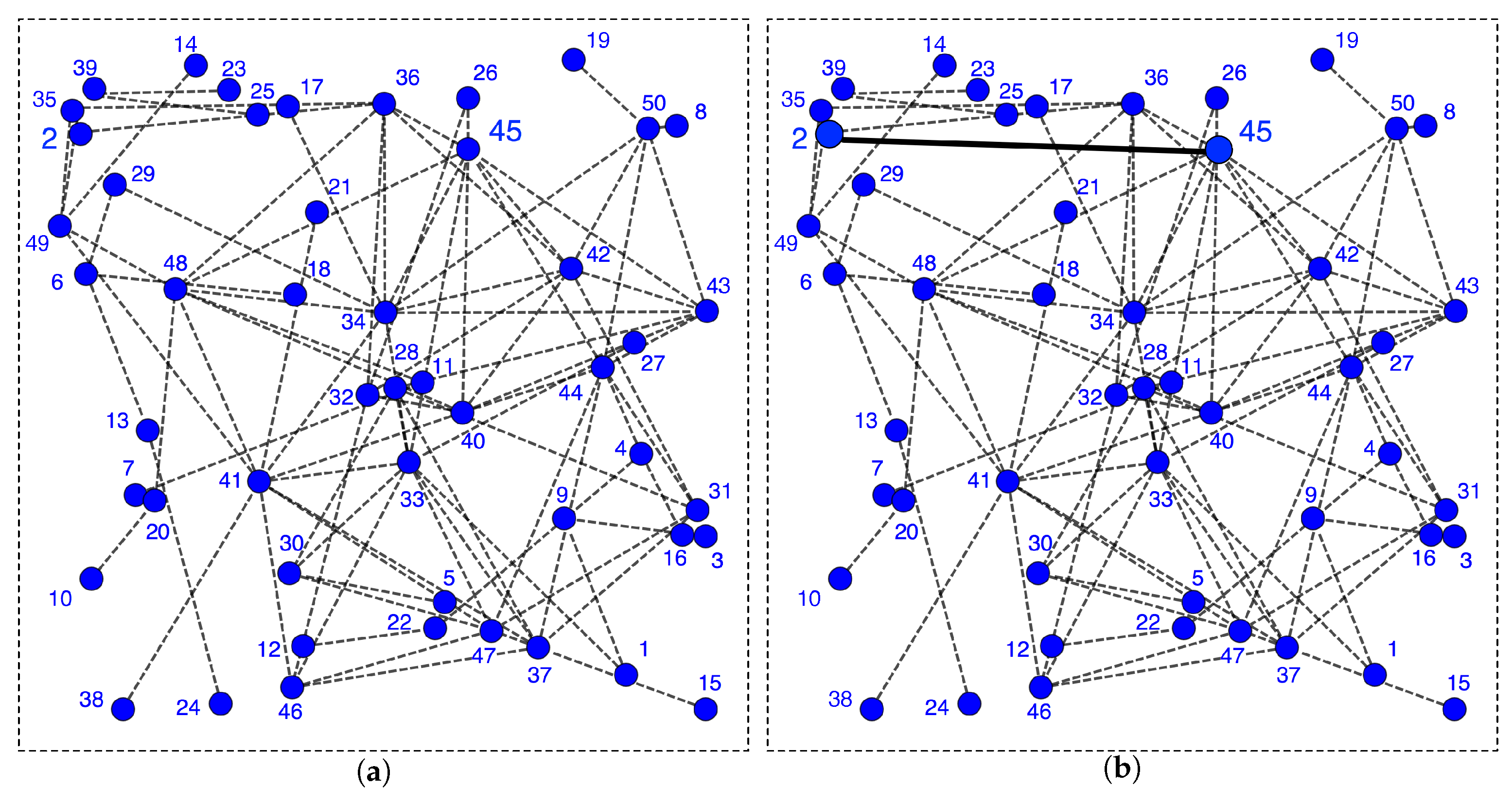
Figure 5 shows some selected results obtained by the proposed EA when minimizing the objective function stated by Equation (11) constrained to Equation (13).

For each value of $\zeta$, the parameter that controls the linear combination of opposing constituents in Equation (11), the problem consists of finding the optimum network (or, equivalently, the optimum graph) that minimizes $f_{\zeta }\left(\mathcal{G}\right)$. The results represented correspond to the mean value (over 20 realizations of the EA).

Figure 5 consists of several subfigures. On the left part of Figure 5, we have represented, as a function of $\zeta$, the following values: (a) the mean value of the objective function, $\overline{f_{\zeta }}$; (b) the multi-scale vulnerability of order two, $b_2$; (c) the average path length, ℓ; (d) the clustering coefficient, $\mathcal{C}$; and (e) the average node degree, $\langle k\rangle$.

On the right part of Figure 5, we have represented some interesting graphs. All of these figures are necessary to properly understand the result. Regarding this, note that:

• The optimum value of $\overline{f_{\zeta }}$ in Figure 5a is achieved for $\zeta =0.7$. This corresponds to the optimum graph ${\mathcal{G}}_{0.7}$ shown in Figure 5h. This graph has $b_2=63$ (Figure 5), which is an intermediate robustness between the one of ${\mathcal{G}}_{0.0}$ (Figure 5f) and that corresponding to ${\mathcal{G}}_{1.0}$ (Figure 5j). ${\mathcal{G}}_{0.7}$ arises from the tradeoff between having a reasonable robustness and efficient power exchange at the local scale (high $\mathcal{C}$ and low ℓ) with a limited number of links ($74\ll 300$, the number of links of ${\mathcal{G}}_{0.0}$). ${\mathcal{G}}_{0.0}$ represents a network with high number of links, very interconnected, and thus, potentially very expensive, and with very high robustness (smallest fragility, $b_2\approx 1$). On the contrary, ${\mathcal{G}}_{1.0}$, which has $b_2\approx 200$, is thus very fragile: note in Figure 5j that the occurrence of abnormal conditions on the marked link will completely disconnect the power grid. In this limiting case ($\zeta =1$), the optimum network ${\mathcal{G}}_{1.0}$ has only 51 links (very low economical cost), but at the expense of being very vulnerable to targeted attacks on hubs.
• A key point to note in Figure 5a is that, in the interval $0.6\le \zeta \le 0.8$, the objective function has a slight variation $80\le \overline{f_{\zeta }}\le 81$, in which the corresponding optimum graphs ${\mathcal{G}}_{0.6}$, ${\mathcal{G}}_{0.7}$ and ${\mathcal{G}}_{0.8}$ exhibit some beneficial properties for the smart grid:

  (a)

  Intermediate robustness, ranging from 50 to 80 in Figure 5b.

  (b)

  A small average path length, $\ell <{\ell }_{\mathrm{RG}}$ (Figure 5c). This is related to the efficient power flow between nodes [30].

  (c)

  Clustering coefficient considerably higher than that of the random graph (with the same number of nodes and links), $\mathcal{C}>{\mathcal{C}}_{\mathrm{RG}}$ (see Figure 5d). This is related to the local exchange of power between neighbor nodes [30]. These two latter conditions are topological features that help the power grid be a smart grid. Furthermore, the two latter features show that the graphs in $0.6\le \zeta \le 0.8$ have the small-world nature. In particular, these graphs with $M\sim 1.66N$ approach non-sparse small-world networks (with $M\sim 2N$), which, according to [76], are the most robust.

  (d)

  Additionally, in $0.6\le \zeta \le 0.8$, $\mathcal{C}\approx 5\times {\mathcal{C}}_{\mathrm{RG}}$, in good agreement with the properties described in [30].

  (e)

  The average node degree $\langle k\rangle$ has values $\approx 3$, which has been proven to be beneficial in [30].

  (f)

  $k_{\mathrm{MAX}}$ ranges between $\approx 5$ and $\approx 7$, which limits the existence of nodes with many links, and therefore, with high capacity (≈ more expensive).

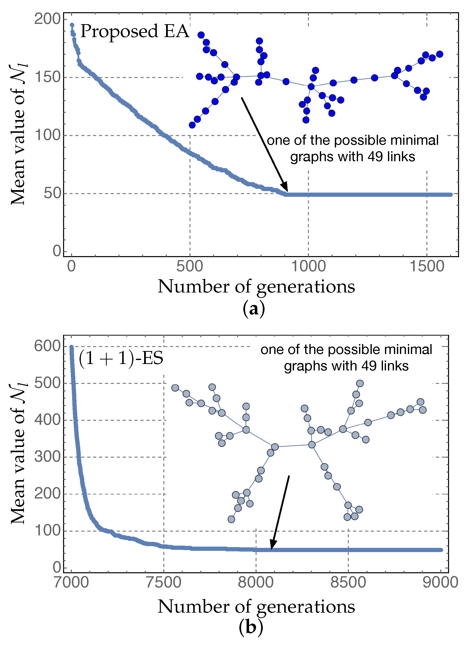
8.3. The Benefits of Adding Links

In this case, we assume that the SG is a network whose nodes are embedded in space (“spatial network” (SN)). This is a realistic condition that appears in some real power grids: the Florida high-voltage power grid, which has been found to be a spatial network with strong geographical constrains that embeds it in space [121], or the Italian power grid [111]). Furthermore, the recent work [122] assumes that a power grid is well described by a two-dimensional, spatially-embedded, connected network. To make the study as general as possible, we assume that the SG is a spatial network whose 50 nodes are located at positions that have been generated at random inside the unit square, with the restriction that the normalized Euclidean distance between any pair of nodes fulfills $d_E(n_i,n_j)\le d_{\mathrm{MAX}}=0.5$.

The purpose of our example is to study the beneficial properties of adding links. In this respect, Figure 6 shows the network obtained by minimizing the number of links constrained to a limit, small algebraic connectivity ${\lambda }_2^{\mathrm{OBJ}}=0.01$, which prevents the network from being disconnected. An initially completely-connected network is the most robust network having the maximum number of links. However, in a real-world infrastructure (such as the power grid), this is unrealistic because of not only economic considerations, but also from a technical viewpoint (substations having many connections). Figure 6 shows the beneficial properties of adding links. By adding only one link between Node 2 and Node 45, the algebraic connectivity increases up to ${\lambda }_2=0.1005$, almost by a factor of $\times 100$, while ℓ increases up to $\ell =3.9⪉3.91=log\left(50\right)$, reaching the corresponding small-world feature.

This results is in good agreement with others found in the literature. The smart addition of links in power grids may lead to the small-world property, making networks more robust [93,96]. Specifically, the survey in [33] shows that the addition of links improves robustness in real grids in Spain, France and Italy [111]. Under the assumption of a small-world WS network model, it is observed that line congestion decreases as the density of shortcuts rises. By rewiring shortcut lines under a certain probability, the mean load in lines results in being lower and so does the number of congested lines. A similar result has been found in [93], which in turn reinforces the suitability of small-word network models when it comes to robustness [73,123,124,125,126].

The advantages arising from small-world diameters has been recently emphasized in [96], in which the system has been modeled as a network of networks, leading to two important conclusions that could help increase robustness (reduce vulnerability). The first one, as mentioned, is that networks with a small diameter are very robust. This has very important practical implications from an engineering viewpoint. In wireless networks, this helps reduce power consumption. In electric grids, this means that generators should be placed near consumers, which can be attained by means of distributed renewable energy generation. This strategy could reduce the investment of deploying or upgrading power transmission grids. The second key conclusion is that adding links is, in general, beneficial until a critical number of lines is reached, beyond which adding more links could increase cascading failures [86]. Note that not all models are consistent regarding the beneficial aspects of adding lines, although it is true that the vast majority of them agree on the conclusion that this strategy is advantageous [33].

Small-sized, small-world topologies for SGs, like those previously obtained, exhibit an additional bonus of helping the intentional islanding. This is a strategy that aims to stop the initial failure occurring in a small part of a power grid [127,128,129] and to prevent it from propagating through the rest of the system, causing thus a larger blackout. In [110,130], the authors suggest that a feasible method to prevent the propagation of disturbances would be to design the network so as to allow for intentionally separable, stable, small islands or “micro-grids”. In the case of emergency, a micro-grid is simply a subset of the grid that can be islanded and which is able to supply electric energy to all or most of its users when an emergency is triggered [33,131]. In this regard, the SG concept can be a good strategy to put this into practice. In a broader approach, a “hybrid” grid is understood as the coexistence of largely interconnected grids with central control and smaller, decentralized areas that could be operated as micro-grids, in the case of emergency. In this context, small, distributed, smart grids as complex networks are on the rise [16,31,48,50], towards an electric grid characterized by a very considerable influence of prosumers, which will have a considerable influence on the electricity distribution infrastructure in the near future.

8.4. Comparison with an Evolution Strategy

The use of an evolutionary algorithm to jointly minimize the link density and the average distance in complex networks was studied in the pioneering, seminal work [132], generating different topologies of general application. This algorithm consists basically of an evolution strategy (ES). The simplest ES works on a population of size two: the current single parent and the result of its mutation. This is the so-called $(1+1)$-ES [133]. The $(1+1)$-ES starts with a single individual (${\mathcal{P}}_{\mathrm{size},\mathrm{initial}}=1$), a graph generated at random. This single progenitor is then evolved by applying a mutation algorithm, which flips an element $a_{ij}$ and generates a new individual. The only constraint is that the resulting mutated network is connected. The objective function is then evaluated with the novel individual. If this value is lower than that of the single progenitor, the new individual is accepted, and the ancestor is removed. Otherwise, the mutant individual is eliminated. This minimization algorithm is iterated until convergence is reached. Figure 7 will assist us with comparing this $(1+1)$-ES to the proposed EA.

Figure 7 shows the mean value of ${\mathcal{N}}_l$ as a function of the number of generations, computed, respectively, by using the proposed EA (a) and the $(1+1)$-ES (b). In this case study, we have considered the number of links (or network size) ${\mathcal{N}}_l$ as the objective function to be minimized because: (1) it is a function in which the exact solution is known; and (2) it is a simple function that requires a much lower computational burden than the one studied above. These two properties make this simple case study allow for obtaining a feasible comparison between the efficiency of the proposed EA and that of the $(1+1)$-ES. We use as the comparative criterion the number of generations necessary for each algorithm to converge to the exact, known solution ${\mathcal{N}}_{l,\min }=M-1$. The results have been represented in Figure 7 for a network with order $M=50$ nodes.

Figure 7 reveals that the $(1+1)$-ES needs a much longer convergence time than that of the proposed EA. Using the number of generations as the comparative criterion, the proposed EA converges to the exact solution (a graph with 49 links) after 900 generations, while the $(1+1)$-ES requires about 8100 generations to converge to a connected graph with the minimum number of links (49 links). That is, the proposed EA is more efficient in the sense that it needs a number of generations $\approx 9$-times lower than that of the simplest $(1+1)$-ES. This is because the latter performs a completely random search ($p_{\mathrm{mut},(1+1)-\mathrm{ES}}=1$) and starts with an initial population with a single progenitor, as long as the EA starts with a larger population (50 individuals) with greater variability and takes advantage of applying a crossover operator (with probability $p_{\mathrm{selec}}=0.8$) in addition to a mutation operator with small probability ($p_{\mathrm{mut}}=0.09$), preventing thus a completely random search.

9. Summary and Conclusions

This paper has focused on describing a method that allows for optimizing the structure of a smart grid (SG) with renewable energy (RE) generation against abnormal conditions (imbalances between generation and consumption, overloads or failures arising from the inherent SG complexity) by combining the complex network (CN) and evolutionary algorithm (EA) concepts.

Our approach takes advantage of some important properties of the SG paradigm being based on: a smart grid allows for the bidirectional exchange of electric energy at the local scale and aims at supplying reliable and safe electric power by efficiently integrating distributed RE generators using smart sensing and communication technologies. Thanks to the efficient integration of distributed REs (small-scale photovoltaic systems and small-wind turbines) in the low voltage grid, electricity consumers can also become producers (“prosumers”), helping end-users obtain economic benefits by selling the energy generated in excess. In this context, we have modeled the SG as a undirected graph so that each link (electric cable) allows for the bidirectional exchange of electric energy between nodes (prosumers).

Aiming at optimizing the structure of such SG against abnormal conditions, we have proposed a novel objective function (to be minimized) that combines cost elements, related to the number of electric cables, and several metrics that quantify properties that are beneficial for the SG (energy exchange at the local scale and high robustness and resilience, as shown in [30]). The optimized SG structure is obtained by applying an EA in which the chromosome that encodes each potential graph (or individual) is the upper triangular matrix of its adjacency matrix. This allows for fully tailoring the crossover and mutation operators to such encoding. Since small-networks have been found to be beneficial for SGs [30], we have proposed a domain-specific initial population that includes both random networks and small-world networks. This assists the proposed EA to converge quickly.

The experimental work points out that the proposed method works well and generates an optimum, synthetic, non-sparse-like small-world structure that leads to beneficial properties such as improving both the energy exchange at the local scale and the robustness and resilience. Specifically, the optimum topology fulfills a balance between moderate cost and robustness against abnormal conditions. We have also explored the benefits of adding links to improve the robustness of smart grids, in good agreement with [73,123,124,125,126]

We would like finally to emphasize that the proposed approach should be considered as a high level analysis and planning tool in the effort of estimating to what extent the smart grid topology can suffer from vulnerabilities. It cannot and does not intend to replace the conventional methods used by power engineers. In fact, the low level, detailed design must be carried out using electrical engineering techniques. In this respect, a deep discussion about the controversy still unresolved between the complex network and electrical engineering communities can be found in [33,35,97,103], reference [35] being a clear introduction to complexity science in the context of power grids.

References

1. Bauer, N.; Bosetti, V.; Hamdi-Cherif, M.; Kitous, A.; McCollum, D.; Méjean, A.; Rao, S.; Turton, H.; Paroussos, L.; Ashina, S.; et al. CO2 emission mitigation and fossil fuel markets: dynamic and international aspects of climate policies. Technol. Forecast. Soc. Chang. 2015, 90, 243–256. [Google Scholar]
2. Peters, G.P.; Andrew, R.M.; Boden, T.; Canadell, J.G.; Ciais, P.; Le Quéré, C.; Marland, G.; Raupach, M.R.; Wilson, C. The challenge to keep global warming below 2 °C. Nat. Clim. Chang. 2013, 3, 4–6. [Google Scholar] [CrossRef]
3. Adefarati, T.; Bansal, R. Reliability assessment of distribution system with the integration of renewable distributed generation. Appl. Energy 2017, 185, 158–171. [Google Scholar]
4. Chen, J.; Zhu, Q. A game-theoretic framework for resilient and distributed generation control of renewable energies in microgrids. IEEE Trans. Smart Grid 2017, 8, 285–295. [Google Scholar]
5. Aghajani, G.; Shayanfar, H.; Shayeghi, H. Demand side management in a smart micro-grid in the presence of renewable generation and demand response. Energy 2017, 126, 622–637. [Google Scholar] [CrossRef]
6. Cabrera-Tobar, A.; Bullich-Massagué, E.; Aragüés-Peñalba, M.; Gomis-Bellmunt, O. Review of advanced grid requirements for the integration of large scale photovoltaic power plants in the transmission system. Renew. Sustain. Energy Rev. 2016, 62, 971–987. [Google Scholar]
7. Datas, A.; López, E.; Ramiro, I.; Antolín, E.; Martí, A.; Luque, A.; Tamaki, R.; Shoji, Y.; Sogabe, T.; Okada, Y. Intermediate band solar cell with extreme broadband spectrum quantum efficiency. Phys. Rev. Lett. 2015, 114, 157701. [Google Scholar] [CrossRef] [PubMed]
8. Cetinay, H.; Kuipers, F.A.; Guven, A.N. Optimal siting and sizing of wind farms. Renew. Energy 2017, 101, 51–58. [Google Scholar]
9. Colmenar-Santos, A.; Perera-Perez, J.; Borge-Diez, D.; dePalacio-Rodríguez, C. Offshore wind energy: A review of the current status, challenges and future development in Spain. Renew. Sustain. Energy Rev. 2016, 64, 1–18. [Google Scholar] [CrossRef]
10. Cuadra, L.; Salcedo-Sanz, S.; Nieto-Borge, J.; Alexandre, E.; Rodríguez, G. Computational intelligence in wave energy: Comprehensive review and case study. Renew. Sustain. Energy Rev. 2016, 58, 1223–1246. [Google Scholar]
11. Santos, S.F.; Fitiwi, D.Z.; Cruz, M.R.; Cabrita, C.M.; Catalão, J.P. Impacts of optimal energy storage deployment and network reconfiguration on renewable integration level in distribution systems. Appl. Energy 2017, 185, 44–55. [Google Scholar] [CrossRef]
12. Caramia, P.; Carpinelli, G.; Mottola, F.; Russo, G. An optimal control of distributed energy resources to improve the power quality and to reduce energy costs of a hybrid AC-DC microgrid. In Proceedings of the 2016 IEEE 16th International Conference on Environment and Electrical Engineering (EEEIC), Florence, Italy, 7–10 June 2016; pp. 1–7. [Google Scholar]
13. Kyritsis, E.; Andersson, J.; Serletis, A. Electricity prices, large-scale renewable integration, and policy implications. Energy Policy 2017, 101, 550–560. [Google Scholar] [CrossRef]
14. Salpakari, J.; Lund, P. Optimal and rule-based control strategies for energy flexibility in buildings with PV. Appl. Energy 2016, 161, 425–436. [Google Scholar] [CrossRef]
15. Yang, A.S.; Su, Y.M.; Wen, C.Y.; Juan, Y.H.; Wang, W.S.; Cheng, C.H. Estimation of wind power generation in dense urban area. Appl. Energy 2016, 171, 213–230. [Google Scholar] [CrossRef]
16. Pagani, G.A.; Aiello, M. Power grid complex network evolutions for the smart grid. Phys. Stat. Mech. Appl. 2014, 396, 248–266. [Google Scholar] [CrossRef]
17. Javaid, N.; Javaid, S.; Abdul, W.; Ahmed, I.; Almogren, A.; Alamri, A.; Niaz, I.A. A hybrid genetic wind driven heuristic optimization algorithm for demand side management in smart grid. Energies 2017, 10, 319. [Google Scholar] [CrossRef]
18. Good, N.; Ellis, K.A.; Mancarella, P. Review and classification of barriers and enablers of demand response in the smart grid. Renew. Sustain. Energy Rev. 2017, 72, 57–72. [Google Scholar] [CrossRef]
19. Yoldaş, Y.; Önen, A.; Muyeen, S.; Vasilakos, A.V.; Alan, İ. Enhancing smart grid with microgrids: Challenges and opportunities. Renew. Sustain. Energy Rev. 2017, 72, 205–214. [Google Scholar] [CrossRef]
20. Wang, H.; Huang, J. Joint Investment and Operation of Microgrid. IEEE Trans. Smart Grid 2017, 8, 833–845. [Google Scholar] [CrossRef]
21. Wang, H.; Huang, J. Cooperative Planning of Renewable Generations for Interconnected Microgrids. IEEE Trans. Smart Grid 2016, 7, 2486–2496. [Google Scholar] [CrossRef]
22. Wang, H.; Huang, J. Incentivizing Energy Trading for Interconnected Microgrids. IEEE Trans. Smart Grid 2017, PP, 1. [Google Scholar] [CrossRef]
23. Tan, K.M.; Ramachandaramurthy, V.K.; Yong, J.Y. Integration of electric vehicles in smart grid: A review on vehicle to grid technologies and optimization techniques. Renew. Sustain. Energy Rev. 2016, 53, 720–732. [Google Scholar] [CrossRef]
24. Bahari, H.I.; Shariff, S.S.M. Review on data center issues and challenges: Towards the Green Data Center. In Proceedings of the 2016 6th IEEE International Conference on Control System, Computing and Engineering (ICCSCE), Batu Ferringhi, Malaysia, 25–27 November 2016; pp. 129–134. [Google Scholar]
25. Carpinelli, G.; Mottola, F.; Proto, D.; Varilone, P. Minimizing unbalances in low-voltage microgrids: Optimal scheduling of distributed resources. Appl. Energy 2017, 191, 170–182. [Google Scholar] [CrossRef]
26. Di Fazio, A.R.; Russo, M.; Valeri, S.; De Santis, M. LV distribution system modelling for distributed energy resources. In Proceedings of the 2016 IEEE 16th International Conference on Environment and Electrical Engineering (EEEIC), Florence, Italy, 7–10 June 2016; pp. 1–6. [Google Scholar]
27. Carpinelli, G.; Mottola, F.; Proto, D.; Russo, A. A multi-objective approach for microgrid scheduling. IEEE Trans. Smart Grid 2016, PP, 1–10. [Google Scholar] [CrossRef]
28. Colak, I.; Sagiroglu, S.; Fulli, G.; Yesilbudak, M.; Covrig, C.F. A survey on the critical issues in smart grid technologies. Renew. Sustain. Energy Rev. 2016, 54, 396–405. [Google Scholar] [CrossRef]
29. Tuballa, M.L.; Abundo, M.L. A review of the development of Smart Grid technologies. Renew. Sustain. Energy Rev. 2016, 59, 710–725. [Google Scholar] [CrossRef]
30. Pagani, G.A.; Aiello, M. From the grid to the smart grid, topologically. Phys. Stat. Mech. Appl. 2016, 449, 160–175. [Google Scholar] [CrossRef]
31. Shi, B.; Liu, J. Decentralized control and fair load-shedding compensations to prevent cascading failures in a smart grid. Int. J. Electr. Power Energy Syst. 2015, 67, 582–590. [Google Scholar] [CrossRef]
32. Jiao, Z.; Gong, H.; Wang, Y. A DS Evidence Theory-based Relay Protection System Hidden Failures Detection Method in Smart Grid. IEEE Trans. Smart Grid 2016, PP, 1. [Google Scholar] [CrossRef]
33. Cuadra, L.; Salcedo-Sanz, S.; Del Ser, J.; Jiménez-Fernández, S.; Geem, Z.W. A critical review of robustness in power grids using complex networks concepts. Energies 2015, 8, 9211–9265. [Google Scholar] [CrossRef] [Green Version]
34. Bompard, E.; Luo, L.; Pons, E. A perspective overview of topological approaches for vulnerability analysis of power transmission grids. Int. J. Crit. Infrastruct. 2015, 11, 15–26. [Google Scholar] [CrossRef]
35. Rosas-Casals, M.; Bologna, S.; Bompard, E.F.; D’Agostino, G.; Ellens, W.; Pagani, G.A.; Scala, A.; Verma, T. Knowing power grids and understanding complexity science. Int. J. Crit. Infrastruct. 2015, 11, 4–14. [Google Scholar] [CrossRef]
36. Dörfler, F.; Chertkov, M.; Bullo, F. Synchronization in complex oscillator networks and smart grids. Proc. Natl. Acad. Sci. USA 2013, 110, 2005–2010. [Google Scholar] [CrossRef] [PubMed]
37. Pagani, G.A.; Aiello, M. The power grid as a complex network: a survey. Phys. Stat. Mech. Appl. 2013, 392, 2688–2700. [Google Scholar] [CrossRef]
38. Amin, S.M.; Giacomoni, A.M. Smart Grid as a Dynamical System of Complex Networks: A Framework for Enhanced Security. IFAC Proc. Vol. 2011, 44, 526–531. [Google Scholar] [CrossRef]
39. Wang, Z.; Scaglione, A.; Thomas, R.J. Generating statistically correct random topologies for testing smart grid communication and control networks. IEEE Trans. Smart Grid 2010, 1, 28–39. [Google Scholar] [CrossRef]
40. Athari, M.H.; Wang, Z. Modeling the uncertainties in renewable generation and smart grid loads for the study of the grid vulnerability. In Proceedings of the 2016 IEEE Power & Energy Society Innovative Smart Grid Technologies Conference (ISGT), Minneapolis, MN, USA, 6–9 September 2016; pp. 1–5. [Google Scholar]
41. Wang, Z.; Elyas, S.H.; Thomas, R.J. A novel measure to characterize bus type assignments of realistic power grids. In Proceedings of the 2015 IEEE Eindhoven PowerTech, Eindhoven, The Netherlands, 29 June–2 July 2015; pp. 1–6. [Google Scholar]
42. Barabási, A.L. Network Science; Cambridge University Press: Cambridge, UK, 2016. [Google Scholar]
43. Halim, Z.; Waqas, M.; Hussain, S.F. Clustering large probabilistic graphs using multi-population evolutionary algorithm. Inf. Sci. 2015, 317, 78–95. [Google Scholar] [CrossRef]
44. Datta, D.; Figueira, J.R.; Fonseca, C.M.; Tavares-Pereira, F. Graph partitioning through a multi-objective evolutionary algorithm: A preliminary study. In Proceedings of the 10th annual conference on Genetic and evolutionary computation, Atlanta, GA, USA, 12–16 July 2008; pp. 625–632. [Google Scholar]
45. Bello-Orgaz, G.; Camacho, D. Evolutionary clustering algorithm for community detection using graph-based information. In Proceedings of the 2014 IEEE congress on Evolutionary Computation (CEC), Beijing, China, 6–11 July 2014; pp. 930–937. [Google Scholar]
46. Pagani, G.A.; Aiello, M. Towards decentralization: A topological investigation of the medium and low voltage grids. IEEE Trans. Smart Grid 2011, 2, 538–547. [Google Scholar] [CrossRef]
47. Pagani, G.; Aiello, M. Modeling the last mile of the smart grid. In Proceedings of the 2013 IEEE PES Innovative Smart Grid Technologies (ISGT), Washington, DC, USA, 24–27 Feburary 2013; pp. 1–6. [Google Scholar]
48. Aiello, M.; Pagani, G.A. The smart grid’s data generating potentials. In Proceedings of the 2014 Federated Conference on Computer Science and Information Systems (FedCSIS), Warsaw, Poland, 7–10 September 2014; pp. 9–16. [Google Scholar]
49. Luo, L.; Pagani, G.A.; Rosas-Casals, M. Spatial optimality in power distribution networks. In Proceedings of the 2014 Complexity in Engineering (COMPENG), Barcelona, Spain, 16–17 June 2014; pp. 1–5. [Google Scholar]
50. Pagani, G.A.; Aiello, M. A complex network approach for identifying vulnerabilities of the medium and low voltage grid. Int. J. Crit. Infrastruct. 2015, 11, 36–61. [Google Scholar] [CrossRef]
51. Pagani, G.A.; Aiello, M. Generating realistic dynamic prices and services for the smart grid. IEEE Syst. J. 2015, 9, 191–198. [Google Scholar] [CrossRef]
52. Capodieci, N.; Pagani, G.A.; Cabri, G.; Aiello, M. An adaptive agent-based system for deregulated smart grids. Serv. Oriented Comput. Appl. 2016, 10, 185–205. [Google Scholar] [CrossRef]
53. Luo, L.; Pagani, G.A.; Rosas-Casals, M. Spatial and Performance Optimality in Power Distribution Networks. IEEE Syst. J. 2016, PP, 1–9. [Google Scholar] [CrossRef]
54. Tvrdík, J.; Křivỳ, I. Hybrid differential evolution algorithm for optimal clustering. Appl. Soft Comput. 2015, 35, 502–512. [Google Scholar] [CrossRef]
55. Brucker, P. On the complexity of clustering problems. In Optimization and Operations Research; Springer: Berlin/Heidelberg, Germany, 1978; pp. 45–54. [Google Scholar]
56. Sun, Y.; Zhang, S.; Ruan, X. Community Detection of Complex Networks Based on the Spectrum Optimization Algorithm. In Proceedings of the 2014 2nd International Conference on Software Engineering, Knowledge Engineering and Information Engineering (SEKEIE 2014)); Atlantis Press: Amsterdam, The Netherlands, 2014. [Google Scholar]
57. Liu, J.; Zhong, W.; Abbass, H.A.; Green, D.G. Separated and overlapping community detection in complex networks using multiobjective Evolutionary Algorithms. In Proceedings of the 2010 IEEE Congress on Evolutionary Computation (CEC), Barcelona, Spain, 18–23 July 2010; pp. 1–7. [Google Scholar]
58. Menéndez, H.D.; Barrero, D.F.; Camacho, D. A co-evolutionary multi-objective approach for a k-adaptive graph-based clustering algorithm. In Proceedings of the 2014 IEEE Congress onE volutionary computation (CEC), Beijing, China, 6–11 July 2014; pp. 2724–2731. [Google Scholar]
59. Wen, X.; Chen, W.N.; Lin, Y.; Gu, T.; Zhang, H.; Li, Y.; Yin, Y.; Zhang, J. A maximal clique based multiobjective evolutionary algorithm for overlapping community detection. IEEE Trans. Evol. Comput. 2016, 21, 363–377. [Google Scholar] [CrossRef]
60. Guturu, P.; Dantu, R. An impatient evolutionary algorithm with probabilistic tabu search for unified solution of some NP-hard problems in graph and set theory via clique finding. IEEE Trans. Syst. Man, Cybern. Part B (Cybern.) 2008, 38, 645–666. [Google Scholar]
61. Yan, J.; Gong, M.; Ma, L.; Wang, S.; Shen, B. Structure optimization based on memetic algorithm for adjusting epidemic threshold on complex networks. Appl. Soft Comput. 2016, 49, 224–237. [Google Scholar] [CrossRef]
62. Harrison, K.R.; Ventresca, M.; Ombuki-Berman, B.M. A meta-analysis of centrality measures for comparing and generating complex network models. J. Comput. Sci. 2015, 17, 205–215. [Google Scholar] [CrossRef]
63. Bailey, A.; Ventresca, M.; Ombuki-Berman, B. Genetic programming for the automatic inference of graph models for complex networks. IEEE Trans. Evol. Comput. 2014, 18, 405–419. [Google Scholar] [CrossRef]
64. Fister, I.; Mernik, M.; Filipič, B. Graph 3-coloring with a hybrid self-adaptive evolutionary algorithm. Comput. Optim. Appl. 2013, 54, 741–770. [Google Scholar] [CrossRef]
65. Bensouyad, M.; Guidoum, N.; Saïdouni, D.E. A New and Fast Evolutionary Algorithm for Strict Strong Graph Coloring Problem. Procedia Comput. Sci. 2015, 73, 138–145. [Google Scholar] [CrossRef]
66. Kaveh, A.; Laknejadi, K. A hybrid evolutionary graph-based multi-objective algorithm for layout optimization of truss structures. Acta Mech. 2013, 224, 343–364. [Google Scholar] [CrossRef]
67. Su, R.; Gui, L.; Fan, Z. Topology and sizing optimization of truss structures using adaptive genetic algorithm with node matrix encoding. In Proceedings of the ICNC’09 Fifth International Conference on Natural Computation, Tianjin, China, 14–16 October 2009; Volume 4, pp. 485–491. [Google Scholar]
68. Giger, M.; Ermanni, P. Evolutionary truss topology optimization using a graph-based parameterization concept. Struct. Multidiscip. Optim. 2006, 32, 313–326. [Google Scholar] [CrossRef]
69. Newman, M.; Barabasi, A.L.; Watts, D.J. The Structure and Dynamics of Networks; Princeton University Press: Princeton, NJ, USA, 2006. [Google Scholar]
70. Newman, D. Complex Dynamics of the Power Transmission Grid (and other Critical Infrastructures). Bull. Am. Phys. Soc. 2015, 60. BAPS.2015.MAR.S18.2. [Google Scholar]
71. Caldarelli, G.; Vespignani, A. (Eds.) Large Scale Structure and Dynamics of Complex Networks: From Information Technology to Finance and Natural Science; World Scientific: Singapore, 2007; Volume 2. [Google Scholar]
72. Watts, D.J.; Strogatz, S.H. Collective dynamics of “small-world” networks. Nature 1998, 393, 440–442. [Google Scholar] [CrossRef] [PubMed]
73. Amaral, L.A.N.; Scala, A.; Barthelemy, M.; Stanley, H.E. Classes of small-world networks. Proc. Natl. Acad. Sci. 2000, 97, 11149–11152. [Google Scholar] [CrossRef] [PubMed]
74. Solé, R.V. Redes Complejas: Del Genoma a Internet; Tusquets Editores: Barcelona, Spain, 2009. [Google Scholar]
75. Jamakovic, A.; Uhlig, S. Influence of the network structure on robustness. In Proceedings of the 15th IEEE International Conference on Networks ( ICON), Adelaide, SA, Australia, 19–21 November 2007; pp. 278–283. [Google Scholar]
76. Zhang, Z.-Z.; Xu, W.-J.; Zeng, S.-Y.; Lin, J.-R. An effective method to improve the robustness of small-world networks under attack. Chin. Phys. 2014, 23, 088902. [Google Scholar] [CrossRef]
77. Newman, M.E.; Watts, D.J. Renormalization group analysis of the small-world network model. Phys. Lett. 1999, 263, 341–346. [Google Scholar] [CrossRef]
78. Wang, X.F.; Chen, G. Complex networks: small-world, scale-free and beyond. IEEE Circuits Syst. Mag. 2003, 3, 6–20. [Google Scholar] [CrossRef]
79. Barabási, A.L. The architecture of complexity. IEEE Control Syst. 2007, 27, 33–42. [Google Scholar] [CrossRef]
80. Barabási, A.L.; Albert, R. Emergence of scaling in random networks. Science 1999, 286, 509–512. [Google Scholar] [PubMed]
81. Barabási, A.L.; Albert, R.; Jeong, H. Mean-field theory for scale-free random networks. Phys. A Stat. Mech. Appl. 1999, 272, 173–187. [Google Scholar] [CrossRef]
82. Bompard, E.; Napoli, R.; Xue, F. Analysis of structural vulnerabilities in power transmission grids. Int. J. Crit. Infrastruct. Prot. 2009, 2, 5–12. [Google Scholar] [CrossRef]
83. Arianos, S.; Bompard, E.; Carbone, A.; Xue, F. Power grid vulnerability: A complex network approach. Chaos Interdiscip. J. Nonlinear Sci. 2009, 19, 013119. [Google Scholar] [CrossRef] [PubMed]
84. Bompard, E.; Wu, D.; Xue, F. The concept of betweenness in the analysis of power grid vulnerability. In Proceedings of the COMPENG’10 Complexity in Engineering, Roma, Italy, 22–24 Feburary 2010; pp. 52–54. [Google Scholar]
85. Bompard, E.; Pons, E.; Wu, D. Extended topological metrics for the analysis of power grid vulnerability. IEEE Syst. J. 2012, 6, 481–487. [Google Scholar] [CrossRef]
86. Brummitt, C.D.; Dsouza, R.M.; Leicht, E. Suppressing cascades of load in interdependent networks. Proc. Natl. Acad. Sci. USA 2012, 109, E680–E689. [Google Scholar] [CrossRef] [PubMed]
87. Wang, Z.; Scaglione, A.; Thomas, R.J. The node degree distribution in power grid and its topology robustness under random and selective node removals. In Proceedings of the 2010 IEEE International Conference on Communications Workshops (ICC), Cape Town, South Africa, 23–27 May 2010; pp. 1–5. [Google Scholar]
88. Wang, J.W.; Rong, L.L. Cascade-based attack vulnerability on the US power grid. Saf. Sci. 2009, 47, 1332–1336. [Google Scholar] [CrossRef]
89. Rosas Casals, M.; Corominas Murtra, B. Assessing European power grid reliability by means of topological measures. WIT Trans. Ecol. Environ. 2009, 122, 515–525. [Google Scholar]
90. Solé, R.V.; Rosas-Casals, M.; Corominas-Murtra, B.; Valverde, S. Robustness of the European power grids under intentional attack. Phys. Rev. 2008, 77, 026102. [Google Scholar] [CrossRef] [PubMed]
91. Cui, L.; Kumara, S.; Albert, R. Complex networks: An engineering view. IEEE Circuits Syst. Mag. 2010, 10, 10–25. [Google Scholar] [CrossRef]
92. Pahwa, S.; Scoglio, C.; Scala, A. Abruptness of cascade failures in power grids. Sci. Rep. 2014, 4. [Google Scholar] [CrossRef] [PubMed]
93. Bashan, A.; Berezin, Y.; Buldyrev, S.V.; Havlin, S. The extreme vulnerability of interdependent spatially embedded networks. Nat. Phys. 2013, 9, 667–672. [Google Scholar] [CrossRef]
94. Brummitt, C.D.; Hines, P.D.; Dobson, I.; Moore, C.; D’Souza, R.M. Transdisciplinary electric power grid science. Proc. Natl. Acad. Sci. USA 2013, 110, 12159. [Google Scholar] [CrossRef] [PubMed]
95. Zhu, Y.; Yan, J.; Sun, Y.; He, H. Revealing cascading failure vulnerability in power grids using risk-graph. IEEE Trans. Parallel Distrib. Syst. 2014, 25, 3274–3284. [Google Scholar] [CrossRef]
96. Dewenter, T.; Hartmann, A.K. Large-deviation properties of resilience of power grids. New J. Phys. 2015, 17, 015005. [Google Scholar] [CrossRef]
97. Luo, L.; Han, B.; Rosas-Casals, M. Network Hierarchy Evolution and System Vulnerability in Power Grids. IEEE Syst. J. 2017. [Google Scholar] [CrossRef]
98. Bilis, E.; Kroger, W.; Nan, C. Performance of electric power systems under physical malicious attacks. IEEE Syst. J. 2013, 7, 854–865. [Google Scholar] [CrossRef]
99. Correa, G.J.; Yusta, J.M. Grid vulnerability analysis based on scale-free graphs versus power flow models. Electr. Power Syst. Res. 2013, 101, 71–79. [Google Scholar] [CrossRef]
100. Hines, P.; Blumsack, S.; Sanchez, E.C.; Barrows, C. The topological and electrical structure of power grids. In Proceedings of the 2010 43rd Hawaii International Conference on System Sciences (HICSS), Honolulu, HI, USA, 5–8 January 2010; pp. 1–10. [Google Scholar]
101. Wang, Z.; Scaglione, A.; Thomas, R.J. Electrical centrality measures for electric power grid vulnerability analysis. In Proceedings of the 2010 49th IEEE Conference on Decision and Control (CDC), Atlanta, GA, USA, 15–17 December 2010; pp. 5792–5797. [Google Scholar]
102. Hines, P.; Blumsack, S. A centrality measure for electrical networks. In Proceedings of the 41st Annual IEEE Hawaii International Conference on System Sciences, Waikoloa, HI, USA, 7–10 January 2008; p. 185. [Google Scholar]
103. Luo, L.; Rosas-Casals, M. Correlating empirical data and extended topological measures in power grid networks. Int. J. Crit. Infrastruct. 2015, 11, 82–96. [Google Scholar] [CrossRef]
104. Cotilla-Sanchez, E.; Hines, P.D.; Barrows, C.; Blumsack, S. Comparing the topological and electrical structure of the North American electric power infrastructure. IEEE Syst. J. 2012, 6, 616–626. [Google Scholar] [CrossRef]
105. Albert, R.; Albert, I.; Nakarado, G.L. Structural vulnerability of the North American power grid. Phys. Rev. 2004, 69, 025103. [Google Scholar] [CrossRef] [PubMed]
106. Chassin, D.P.; Posse, C. Evaluating North American electric grid reliability using the Barabási–Albert network model. Phys. Stat. Mech. Appl. 2005, 355, 667–677. [Google Scholar] [CrossRef]
107. Mei, S.; Zhang, X.; Cao, M. Power Grid Complexity; Springer Science & Business Media: Berlin/Heidelberg, Germany, 2011. [Google Scholar]
108. Rosato, V.; Bologna, S.; Tiriticco, F. Topological properties of high-voltage electrical transmission networks. Electr. Power Syst. Res. 2007, 77, 99–105. [Google Scholar] [CrossRef]
109. Holmgren, Å.J. Using graph models to analyze the vulnerability of electric power networks. Risk Anal. 2006, 26, 955–969. [Google Scholar] [CrossRef] [PubMed]
110. Rosas-Casals, M.; Valverde, S.; Solé, R.V. Topological vulnerability of the European power grid under errors and attacks. Int. J. Bifurc. Chaos 2007, 17, 2465–2475. [Google Scholar] [CrossRef]
111. Crucitti, P.; Latora, V.; Marchiori, M. Locating critical lines in high-voltage electrical power grids. Fluct. Noise Lett. 2005, 5, L201–L208. [Google Scholar] [CrossRef]
112. Kim, C.J.; Obah, O.B. Vulnerability assessment of power grid using graph topological indices. Int. J. Emerg. Electr. Power Syst. 2007, 8. [Google Scholar] [CrossRef]
113. Yazdani, A.; Dueñas-Osorio, L.; Li, Q. A scoring mechanism for the rank aggregation of network robustness. Commun. Nonlinear Sci. Numer. Simul. 2013, 18, 2722–2732. [Google Scholar] [CrossRef]
114. Boccaletti, S.; Buldú, J.; Criado, R.; Flores, J.; Latora, V.; Pello, J.; Romance, M. Multiscale vulnerability of complex networks. Chaos Interdiscip. J. Nonlinear Sci. 2007, 17, 043110. [Google Scholar] [CrossRef] [PubMed]
115. Eiben, A.E.; Smith, J. What is an evolutionary algorithm? In Introduction to Evolutionary Computing; Springer: Berlin/Heidelberg, Germany, 2015; pp. 25–48. [Google Scholar]
116. Simon, D. Evolutionary Optimization Algorithms; John Wiley & Sons: Hoboken, NJ, USA, 2013. [Google Scholar]
117. del Arco-Vega, M.A.; Cuadra, L.; Portilla-Figueras, J.A.; Salcedo-Sanz, S. Near-optimal user assignment in LTE mobile networks with evolutionary computing. Trans. Emerg. Telecommun. Technol. 2016. [Google Scholar] [CrossRef]
118. Sastry, K.; Goldberg, D.E.; Kendall, G. Genetic algorithms. In Search Methodologies; Springer: Berlin/Heidelberg, Germany, 2014; pp. 93–117. [Google Scholar]
119. Deng, Y.; Liu, Y.; Zhou, D. An improved genetic algorithm with initial population strategy for symmetric TSP. Math. Prob. Eng. 2015, 2015, 212794. [Google Scholar] [CrossRef]
120. Miller, B.L.; Goldberg, D.E. Genetic algorithms, tournament selection, and the effects of noise. Complex Syst. 1995, 9, 193–212. [Google Scholar]
121. Xu, Y.; Gurfinkel, A.J.; Rikvold, P.A. Architecture of the Florida power grid as a complex network. Phys. Stat. Mech. Appl. 2014, 401, 130–140. [Google Scholar] [CrossRef]
122. Schultz, P.; Heitzig, J.; Kurths, J. A random growth model for power grids and other spatially embedded infrastructure networks. Eur. Phys. J. Spec. Top. 2014, 223, 2593–2610. [Google Scholar] [CrossRef]
123. Han, P.; Zhang, S. Analysis of cascading failures in small-world power grid. Int. J. Energy Sci. 2011, 1, 99–104. [Google Scholar]
124. Latora, V.; Marchiori, M. Efficient behavior of small-world networks. Phys. Rev. Lett. 2001, 87, 198701. [Google Scholar] [CrossRef] [PubMed]
125. Ding, M.; Han, P. Reliability assessment to large-scale power grid based on small-world topological model. In Proceedings of the PowerCon 2006 International Conference on Power System Technology, Chongqing, China, 22–26 October 2006; pp. 1–5. [Google Scholar]
126. Fu, L.; Huang, W.; Xiao, S.; Li, Y.; Guo, S. Vulnerability assessment for power grid based on small-world topological model. In Proceedings of the 2010 Asia-Pacific, IEEE Power and Energy Engineering Conference (APPEEC), Chengdu, China, 28–31 March 2010; pp. 1–4. [Google Scholar]
127. Trodden, P.; Bukhsh, W.A.; Grothey, A.; McKinnon, K. Optimization-based islanding of power networks using piecewise linear AC power flow. IEEE Trans. Power Syst. 2014, 29, 1212–1220. [Google Scholar] [CrossRef]
128. Pahwa, S.; Youssef, M.; Schumm, P.; Scoglio, C.; Schulz, N. Optimal intentional islanding to enhance the robustness of power grid networks. Phys. Stat. Mech. Appl. 2013, 392, 3741–3754. [Google Scholar] [CrossRef]
129. Trodden, P.; Bukhsh, W.; Grothey, A.; McKinnon, K. MILP formulation for controlled islanding of power networks. Int. J. Electr. Power Energy Syst. 2013, 45, 501–508. [Google Scholar] [CrossRef] [Green Version]
130. Carreras, B.A.; Newman, D.; Dobson, I. Does size matter? Chaos Interdiscip. J. Nonlinear Sci. 2014, 24, 023104. [Google Scholar] [CrossRef] [PubMed] [Green Version]
131. Panteli, M.; Mancarella, P. The Grid: Stronger, Bigger, Smarter? Presenting a Conceptual Framework of Power System Resilience. IEEE Power Energy Mag. 2015, 13, 58–66. [Google Scholar] [CrossRef]
132. Cancho, R.F.; Solé, R.V. Optimization in complex networks. In Statistical Mechanics Of Complex Networks; Springer: Berlin/Heidelberg, Germany, 2003; pp. 114–126. [Google Scholar]
133. Beyer, H.G.; Schwefel, H.P. Evolution strategies—A comprehensive introduction. Nat. Comput. 2002, 1, 3–52. [Google Scholar] [CrossRef]
Figure 1. (a) First step in the creation of a small-world Watts–Strogatz (WS) network; (b) example of a WS network and its node degree distribution; (c) scale-free network. See the main text for further details.
Energies 10 01097 g001
Figure 2. Simple example illustrating the encoding process. (a) Small random graph G (or individual) with 10 nodes and 20 links; (b) adjacency matrix A G of graph G ; (c) upper triangular matrix T G or chromosome c G = T G encoding the information of individual G .
Energies 10 01097 g002
Figure 3. Examples of four graphs belonging to the initial population. (a) Watts–Strogatz random graphs; (b) Erdős–Rényi (ER) random graphs.
Energies 10 01097 g003
Figure 4. Mean value (a) and variance (b) obtained by the proposed EA when minimizing the objective function stated by Equation (11) for ζ = 0.7 and constrained to Equation (13), as a function of the number of generations.
Energies 10 01097 g004
Figure 5. Result reached by the proposed EA when minimizing the objective function stated by Equation (11) as a function of ζ : (a) Mean value of the objective function, f ζ ¯ ; (b) Multi-scale vulnerability of order two, b 2 ; (c) Average path length, ; (d) Clustering coefficient, C ; (e) Average node degree, k . On the right side, (f), (g), (h) and (i) show, respectively, optimum structures for several values of ζ : G 0.0 , G 0.6 , G 0.7 and G 1.0 . (j) Summary of illustrative results for G 0.6 and G 0.7 .
Energies 10 01097 g005
Figure 6. (a) Spatial network with minimum algebraic connectivity; (b) addition on a link between Node “2” and Node “45”.
Energies 10 01097 g006
Figure 7. Mean value of the number of links ( N l ) as a function of the number of generation using, respectively, the proposed EA (a) and the ( 1 + 1 ) -evolution strategy (ES) (b). The number of nodes is M = 50 .
Energies 10 01097 g007