
Two-Stage Coordinated Operational Strategy for Distributed Energy Resources Considering Wind Power Curtailment Penalty Cost


1
Commonwealth Scientific and Industrial Research Organization (CSIRO), Mayfield West, Newcastle, NSW 2304, Australia
2
School of Science and Engineering, Chinese University of Hong Kong (Shenzhen), Shenzhen 518172, China
3
Centre for Intelligent Electricity Networks, University of Newcastle, Newcastle, NSW 2308, Australia
4
Electric Power Research Institute, CSG, Guangzhou 510080, China
*
Author to whom correspondence should be addressed.
Energies 2017, 10(7), 965; https://doi.org/10.3390/en10070965
Submission received: 4 May 2017
/
Revised: 26 June 2017
/
Accepted: 7 July 2017
/
Published: 10 July 2017
(This article belongs to the Section F: Electrical Engineering)
Abstract
:The concept of virtual power plant (VPP) has been proposed to facilitate the integration of distributed renewable energy. VPP behaves similar to a single entity that aggregates a collection of distributed energy resources (DERs) such as distributed generators, storage devices, flexible loads, etc., so that the aggregated power outputs can be flexibly dispatched and traded in electricity markets. This paper presents an optimal scheduling model for VPP participating in day-ahead (DA) and real-time (RT) markets. In the DA market, VPP aims to maximize the expected profit and reduce the risk in relation to uncertainties. The risk is measured by a risk factor based on the mean-variance Markowitz theory. In the RT market, VPP aims to minimize the imbalance cost and wind power curtailment by adjusting the scheduling of DERs in its portfolio. In case studies, the benefits (e.g., surplus profit and reduced wind power curtailment) of aggregated VPP operation are assessed. Moreover, we have investigated how these benefits are affected by different risk-aversion levels and uncertainty levels. According to the simulation results, the aggregated VPP scheduling approach can effectively help the integration of wind power, mitigate the impact of uncertainties, and reduce the cost of risk-aversion.
1. Introduction
Virtual power plant (VPP) is termed as a single entity that integrates the portfolio of different types of distributed energy resources (DERs) [1,2]. The integration can make the summed capacity of many diverse small-scale DERs be large enough to trade energy or provide network support services in pool markets. Meanwhile, VPP creates a single operating profile from a composite of the parameters characterizing each DER [3,4]. This aggregation enhances the visibility and controllability of DERs to system operators and other market participants [5,6]. Specifically, VPP integrates various types of renewable and nonrenewable generators, storages and flexible loads [7,8]. The weakness and strength of different DERs are combined in a complementary way, thus enabling cost-efficient, secure and sustainable energy supply systems [9,10]. Moreover, depending on the net power between production and demand, VPP can be a producer or a consumer (i.e., a prosumer). The profit variability in electricity markets becomes the major concern and VPP should optimize the scheduling of DERs and bid/offer more strategically [11]. Given the market risks in relation to uncertainties, sophisticated risk management strategies are also needed [9].
In the literature, reference [10] has proposed an optimal operation model for VPP participating in both day-ahead (DA) and balancing markets. The model is formulated as a mixed-integer linear programming (MILP) problem, while the conditional value at risk (CVaR) is used as a measure to control the risk of low profit scenarios. In [12], the optimal offering of VPP in the DA and balancing markets is also modeled as an MILP problem, aiming to maximize the expected profit. In [9], the participation of VPP in the DA and real-time (RT) markets is modeled by a stochastic Game theory approach. CVaR is used to compute risks due to uncertainties. In [1], the bidding strategy for VPP in energy and ancillary (spinning reserve services) markets is addressed. The optimal bidding problem is formulated as a single level non-equilibrium model based on the deterministic price-based unit commitment (PBUC). In [13], a stochastic bi-level approach is adopted to address the optimal bidding strategy for VPP. The bi-level problem is formulated as an MILP problem based on the Karush–Kuhn–Tucker optimality conditions and the strong duality theory. Nezamabadi et al. [14] proposed an arbitrage strategy for VPP participating in energy and ancillary markets. The proposed model is based on a security-constrained PBUC, aiming to maximize the profit considering arbitrage opportunities. Similarly, Karimyan et al. [15] used the PBUC method to identify the optimal operation of VPP in energy and reserve markets. The problem is formulated as a mixed-integer nonlinear programming (MINLP) problem, which is solved by the particle swarm optimization (PSO) algorithm. Luo et al. [16] has proposed a two-stage operational planning framework for VPP. The first stage optimizes VPP hourly scheduling in the energy market, while the second stage optimizes the RT control actions using a model predictive control-based dispatch model. Vasirani et al. [17] proposed an agent-based approach to optimal operations of VPP. The model is based on linear programming, and the interactions between the grid and electric vehicle (EV) batteries are investigated.
Most of the above-mentioned references use simplified linear models, and hence the network constraints have been neglected and some important system parameters such as reactive power are not taken into account. On the other hand, some references have not well addressed the risks for VPP participating in pool markets or failed to characterize the correlations between uncertainties (e.g., load, price or wind power availability). By contrast, in this paper, we have proposed an optimal scheduling model for a price-taker VPP participating in the DA and RT balancing markets. The complex network flow constraints and the unit commitments of DERs are explicitly taken into account, thus making the proposed model more applicable in practice. In addition, to comprehend the profit variants in markets, a risk factor is introduced into the optimal scheduling formulation based on the mean-variance Markowitz theory [18]. As a result, value-at-risk (VaR) becomes the model output in this paper, rather than a part of the objective function as reported in [19]. Moreover, the benefits of coordination (VPP aggregation) and the corresponding sensitivity analysis are demonstrated in case studies.
The remainder paper is organized as follows: in Section 2, the problem description is given, followed by proposed optimal scheduling model for VPP in Section 3. Section 4 introduces the applied solution algorithm. Section 5 presents numerical simulations to demonstrate the effectiveness of the proposed approach. Conclusions are given in Section 6.
2. Problem Formulation
As seen in Figure 1, DERs such as battery energy storage system (BESS) units, distributed generation (DG) units (thermal), wind power and solar generators, and end consumers (both interruptible and non-interruptible loads) are physically interconnected to the upstream distribution networks. It should be noted that unlike a microgrid a VPP is not necessarily limited to a geographical location [2]. VPP acts as a representative that manages all transactions of DERs with the independent system operator (ISO). In other words, the VPP needs to submit hourly scheduling plans in energy markets. Thus, VPP is exposed to the market risk and needs to optimize its scheduling based on the entire portfolio’s operational constraints and the system-state estimation [10]. Moreover, end consumers of VPP are supplied with a given retail energy rate, and they are not exposed to the price volatility in spot energy markets [7]. VPP signs a contract with interruptible consumers, in which the upper limit and cost of load curtailment are specified. DG and BESS may be used for trading energy but corresponding costs should be paid. The operational cost of wind power is assumed to be negligible.
The market structure studied in this work is a joint DA and RT electricity markets, which is common in European electricity pools such as Nord Pool [16]. In the DA (spot) market, participants propose their scheduling for each hour of the coming day before the gate closure. After the spot price has been settled and commitments have been made, participants are responsible for deviations due to unpredictable fluctuations in power production or consumption. In the RT market, any deviation from the commitment made in the DA market will be settled by a regulation price. If the actual consumption is more than (or the production is less than) the commitment, the power shortage is purchased at an up-regulation price, which is usually higher than the spot price. If the actual consumption is less than (or the production is more than) the commitment, the power surplus is sold at a down-regulation price, which is usually lower than the spot price [13]. As a result, this market structure encourages participants to reduce their forecast errors and be more strategic in operations [20].
In the above-mentioned market framework, three assumptions are made for the operation of VPP: (i) DERs in VPP are centrally controlled [1]. This means the VPP central controller is responsible for bi-directional communication, monitoring, and control of each VPP component; (ii) VPP can obtain the required data for managing its portfolio (e.g., price and load data). The relevant time-series forecast techniques are available; (iii) VPP is considered as a price-taker, which means its operational strategy dose not influence the market price.
3. Optimal Scheduling of VPP
3.1. Key Models
3.1.1. Price Model
In the DA market, the VPP schedules the hourly power (i.e., quantity of power consumption or production) for the next trading day. If , VPP is a producer; if , the VPP is a consumer. Because of the variations of power production and load, there will be a deviation between the scheduling and the forecasted power. The deviation at time is:
where denotes the forecasted power to be traded.
Thus, the imbalance cost is calculated as:
where and denote regulation prices for purchasing (up-regulation) and selling (down-regulation) electricity in real-time balancing market at time , respectively.
In addition, in the particular markets, we assume that the regulation price can be calculated as proportions of the DA market price :
where and denote the relative differences between the day-ahead price and the up-regulation/down-regulation prices.
Therefore, market price uncertainty can be modeled by a random vector, including random DA price and random differences between DA up and down regulation prices. The distributions of market prices can be obtained by a variety of time-series based forecasting techniques such as autoregressive integrated moving average (ARIMA), which have been well addressed in [21,22].
3.1.2. Interruptible Load (IL) Cost Model
The cost of IL is assumed to be a function of adjusted load at time bus , and is modeled by a quadratic polynomial function as [1]:
where , denote cost coefficients of IL. It should be noted that negative IL (i.e., load increase) also exists for balancing underestimated renewable energy outputs. An example of the upward demand response (DR) could be the controllable electric vehicle (EV) loads through the vehicle-to-grid (V2G) technology.
3.1.3. BESS Cost Model
The operational cost of BESS at time bus generally refers to maintenance cost [16], which can be modeled by a linear function as:
where denote the charged or discharged BESS power at time bus ; denotes energy stored in BESS; denotes a factor that converts power (kW) to energy (kWh), i.e., time duration; denote leakage loss factor of BESS; and is the cost coefficient of the BESS lifetime depression, which is calculated as [23]:
where , , and denote investment cost, rated energy capacity and total life cycle number of BESS.
3.1.4. DG Cost Model
DG can refer to any kind of DERs though, in this paper DG is only termed as distributed thermal units (e.g., diesel or gas fired power generators), in order to distinguish it from wind power units. The cost of DG can be modeled by a quadratic function of its real power output [24]:
where , , and denote cost coefficients of DG at bus ; and denotes DG output at bus time .
3.1.5. Model of Other Uncertainties
In this paper, load, market price, and wind speed are considered as uncertainties. The historical data in the DA market is used as correlated scenarios, and hence the correlated probability distributions can be estimated based on the statistical correlations among these uncertainties. More detailed information can be found in [21], which comprehensively discusses a variety of time-series-based methods to generate correlated scenarios. In this paper, the ARIMA method is used to generate correlated time-series wind speed, load and price data. To model the forecast errors produced by the ARIMA model, Monte Carlo (MC) simulations are used to sample scenarios. In general, load forecast errors and market price forecast errors can be modeled by the Gaussian distribution [3]. Wind speed can be modeled by the Weibull distribution [16,25].
3.2. Day-Ahead Scheduling
In the DA market, VPP optimizes its hourly scheduling and unit commitments to maximize the total profit over the scheduling horizon. Meanwhile, the decision made in this stage may affect its operational strategies in the RT market. Thus, it is necessary to consider the decision variables pertaining to the RT market while optimizing the scheduling in the DA market. However, note that the RT market decision variables are not actually implemented in the DA market.
The optimal scheduling model of VPP in the DA market is formulated as:
where denotes the retail price agreed between VPP and the customers; denotes the forecasted load at time ; and denote start-up (usually including cold and hot start-up costs) and shut-down costs of DG, respectively; denote the total DA scheduling horizon (e.g., 24 h); , , and are binary variables denoting commitment status, start-up and shut-down decisions for DG at time bus , respectively; and , , and denote sets of BESS, DG and demand, respectively. In Equation (8), the first term represents the cost (revenue) of VPP by purchasing (selling) electricity from (to) the distribution system. The second term represents the revenue by selling electricity to the customers. The remaining terms in Equation (8) represent costs of power imbalance, IL, BESS and DG. The retail price in this paper is set according to the residential energy time-of-use (TOU) price in New South Wales, Australia. Specifically, the peak price is 48 cent/kWh, the shoulder price is 19.50 cent/kWh and the off-peak price is 12 cent/kWh.
Given the uncertainties in electricity markets, a decision-making can be risky. Moreover, Equation (8) should be formulated as a probabilistic version. To enhance the computational efficiency, the initial set of scenarios is reduced to a number of representative scenarios using an appropriate scenario reduction technique such as adaptive importance sampling presented in [26]. Moreover, the risk associated with the profit variability is explicitly captured into the model through the mean-variance Markowitz theory [18]. Thus, Equation (8) is rewritten as:
where denotes the expected profit; denote the standard deviation; is a weighting factor for the incorporation of risk in the objective function [27]. Higher values of indicate greater risk aversion. Particularly, means an absolute risk-neutral strategy. The calculation of Equation (9) is given in Equations (10) and (11).
where denotes the probability of scenario ; and denotes the set of total scenarios. The probability of scenario is obtained as follows. We firstly use the ARIMA model to generate correlated uncertainty data such as load, price, and wind speed. The parameters of the ARIMA are obtained based on the historical data in Nord Pool in 2015. Afterwards, the Monte Carlo (MC) simulations are used to generate uncertainty forecast errors produced by the ARIMA model. The probability of each scenario () is obtained based on the histogram of the sampled correlated scenarios in MC simulations. The total number of scenarios is the bin size. The values of scenarios are the mean of samples in the corresponding bin. Lastly, the scenarios are used as model inputs to calculate the objective in Equation (8), which is . The larger is the bin size, the more accurate is the result.
For each scenario, the complete constraints of Equation (9) are given below.
3.2.1. Supply-Demand Balance Constraint
3.2.2. Wind Power Constraint
3.2.3. DG Constraint
3.2.4. IL Constraint
Equation (19) states the maximum ratio of IL, i.e., .
3.2.5. BESS Constraint
3.2.6. Network Constraint
To accurately model the power losses and reactive power, the alternating current (AC) power flow model is used as follow.
where and denote active and reactive power injection time bus scenario ; and denote active and reactive power generation, while and denote active and reactive power demand; denotes complex power flow between at time , with voltage angle and amplitude ; and denotes set of all buses.
3.2.7. Interconnection Exchange Constraint
Equation (30) states that is within the upper and lower limits of interconnection exchange between VPP and the upstream grid.
3.2.8. Steady Security Reserve Constraint
Equation (31) states the system reserve requirement for static security and adequacy [1]. The system reserve requirement is assumed to be 1.5 times the total system peak load.
3.3. Real-Time Balancing
The real-time dispatch is to maintain the power balance. Because of the forecast errors of uncertainties, any deviation from the commitment made in the DA market should be balanced. The smaller is the RT dispatch interval, the smaller are the forecast errors. Thus, the frequency of RT clearing is very high (e.g., 5-min). Time-series forecast techniques such as ARIMA are appropriate to capture the persistent behavior of uncertainties [22]. Moreover, the last slight imbalances in each dispatch interval can be handled by automatic generation control and/or emergency DR (i.e., instantaneous control).
The objective of VPP in the RT market is to minimize the imbalance cost and wind power curtailment. In this particular market, we assume that the curtailment of wind power will be published by a monetary penalty coefficient, as given below.
where denotes total number of dispatch intervals in the RT market; denotes imbalance cost due to production and consumption variations in the RT market; is the penalty price of wind power curtailment; and is the available wind power at time bus .
Note that we simply use to distinguish the variables in the RT market from the variables in the DA market. The detailed calculations of are given in Equations (33)–(35).
The constraints of Equation (32) include Equation (12)–(15), (19)–(23), and (25)–(30).
4. Solution Algorithm
4.1. Solution to the DA Scheduling Problem
The hourly DA scheduling of VPP is a mixed-integer nonlinear programing problem. The model is a here-and-now decision-making process, meaning that decisions are made prior to the knowledge of uncertainty data such as wind speed, load and price data [28]. The decision variables in Equation (9) include , , , , , , , , . The mathematical programming methods are not suitable for solving this problem, since the formulated VPP scheduling model is a nonlinear and non-convex optimization problem. By contrast, the heuristic-based optimization methods are free from the problem complexity [1,29]. In this paper, the differential evolution (DE) is employed to solve the upper level optimization model. The computational efficiency of this algorithm has been demonstrated in [30]. The applied solution algorithm is briefly introduced below.
(1) Input data
Input data such as network, wind speed, load, price, etc.
(2) Initialization
Start the DE algorithm, generate an initial population randomly, and set the objective function value . Note that, here, denotes the population size, which is the number of generated candidate solutions (called individuals) in each iteration. The more individuals there are in the population, the more differential vectors are available. As a result, the more directions can be explored. However, the computational complexity per generation increases with the size of the population.
(3) Check constraints and calculate the fitness value
For the population size , perform the following steps:
Section 3.1: Check the operational requirements by running power flow functions. The ON/OFF commitment constraint handling algorithm in [31] is applied to adjust the binary states of DG and BESS to satisfy Constraints (15)–(18) and (20)–(25). Based on the given values of DG output , BESS output and IL amount , the power flow function [32] is run to calculate the VPP power losses and the value of exchanged power with the upstream power grid. The exchanged power is equal to the scheduled power . In addition, other constraints such as the network security and adequacy constraints (Equations (26)–(29)), the interconnection constraint (Equation (30)) and the reserve constraint (Equation (31)) are checked based on running the power flow function. Furthermore, after obtaining the power flow results for all scenarios, the expected profit and its standard deviation are calculated using (9)–(11).
Section 3.2: If there is any violation of the above-mentioned constraints, a variable penalty is assigned. The variable penalty is defined as a function of the distance from the feasible area [1]. The summation of absolute distances of violated constraints is scaled by a large penalty factor and then is combined with the objective function to constitute the fitness. By doing so, infeasible solutions are not discarded. Instead, their information can be used to guide the algorithm search [1].
(4) Update the best individual and selection
Find and update the best individual of the current generation. This step involves comparing individuals with each other. The fitness sharing technique proposed in [30] is used to select the best one whose fitness value is the highest.
(5) Offspring generation
Produce the offspring generation according to the evolution rule in DE. Typical evolution operations include mutation, recombination and crossover. Detailed mathematical formulations of offspring generation can be found in [30,33].
(6) Termination
If any stopping criterion is met, e.g., the fitness value doses not improve in a number of successive iterations, stop and export the best individual. Otherwise, go back to Step 3.
4.2. Solution to the RT Balancing Problem
After solving the optimal scheduling model in the DA, the ON/OFF states of DERs are determined. VPP needs to reschedule DERs in real-time (e.g., on a five-minute basis) to compensate the energy deviations incurred. The lower level optimal operation model is a nonlinear programming problem with continuous variables. Variables such as , , are wait-and-see decisions, meaning that decisions can be made when the information about the future is already known [28]. The flow chart of the applied solution algorithm in two stages is shown in Figure 2. We use the solver AMPL/IPOPT 3.8.0 (900 Sierra Place SE, Albuquerque, NM, USA) to solve the RT balancing. This solver is called Interior Point Optimizer, which is based on a mathematical programming algorithm called the interior point method. This method adopts barrier functions to achieve optimization by going through the middle of the solid defined by the problem rather than around its surface.
5. Case Studies
5.1. Experimental Setting
The proposed VPP scheduling approach is tested on a real 12-bus distribution system of the CSIRO energy center in Newcastle, Australia. The VPP scheduling models are coded in MATLAB® (R2015b, Chatswood, Australia). As seen in Figure 3, the system is comprised of 4 wind turbines, 3 BESS, 3 DG units, and 11 load buses. The total generation capacity is 6500 kW, including 3000 kW of wind power and 3500 kW of DG. We assume that IL is located at every load bus, and up to 10% of the system load can be adjusted if necessary. The corresponding IL costs are composed of three bands, i.e., early morning (first 6 h), day time (middle 12 h) and evening (last 6 h). The capacity of power interconnection between VPP and the main grid is set as 4000 kW. The power curve of a Vestas V27 wind turbine is used [16]. The rated, cut-in, and cut-out wind speeds are 14.0, 3.5 and 25.0 m/s, respectively. The start-up and shut-down costs of DG are assumed to be $70 and $20, respectively. In the base case, the weighting factor is set to be 0.1. The correlated scenarios of market price, wind speed, and demand are modeled based on the Nord Pool historical data in 2015, which are publically available on [34]. Note that the data have been scaled down and monetary units are transferred to US$. The historical wind power production data in Denmark are used. The wind power output is calculated using the power-speed curve as [35]:
where and denote wind power output and wind speed, respectively; , , and denote cut-in, cut-out and rated wind speeds, respectively; and denotes rated wind power.
5.2. Results and Discussion
To verify the effectiveness of the proposed model, two cases are compared. Case 1: An uncoordinated operation strategy. Individual VPP element operates strategically as a price-taker in the DA market, aiming to maximize their profits. The total profit is the summation of individual’s profit virtually obtained [12]. The imbalance cost is calculated after the realization of scenarios. Case 2: The proposed integrated VPP scheduling approach.
The profit distributions in the DA market for Cases 1 and 2 are illustrated in Figure 4. Compared to Case 1, the expected profit for Case 2 is higher ($4595.50 for Case 1 and $5823.30 for Case 2); while the standard deviation (Std.) for Case 2 is relatively lower. In addition, we use the Value-at-Risk (VaR) at a confidence level of 95% to evaluate the risk of different operational strategies. In other words, the VaR-95% denotes the expected value of the 5% scenarios with lowest profit. As seen in Figure 4, the VaR is $2506.20 and $3485.60 for Cases 1 and 2, respectively. This implies that Case 2 incurs less risk in the DA market.
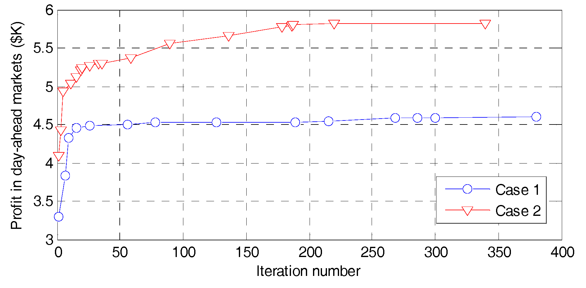
The iteration convergences of DE for Cases 1 and 2 are illustrated in Figure 5. We can see that the DE solution algorithm requires 381 and 342 iterations for Cases 1 and 2, respectively, corresponding to computational time periods of 1982 and 1671 seconds on a PC with Intel Core i7-6600 CPU @ 2.80 GHZ with 8.00 GB RAM.
Moreover, the energy stored in BESS and the dis/charged power in the DA and RT markets are shown in Figure 6. In both cases, BESS is charged in the early morning (e.g., 2–4 a.m.) or late afternoon (2–4 p.m.). BESS is discharged to satisfy the morning and evening peaks, when electricity prices are relatively higher. In other words, the profits made by BESS are based on the price differences between off-peak and on-peak periods. It is worth mentioning that power deviations in the two markets for Case 1 are smaller than Case 2. For the uncoordinated operation in Case 1, BESS only faces load uncertainty (i.e., load forecast errors). By contrast, for the aggregated VPP operation, BESS is required to cover the risks faced by other types of DERs and hence more power fluctuations are observed in Case 2. For instance, wind availability poses a significant risk to WP and WP is free from the market price volatility (generation cost for VPP is zero). On the contrary, wind availability is not an issue for thermal DG units, but DG operations are greatly influenced by market prices. Meanwhile, load uncertainty has more direct impacts on BESS and IL. Therefore, the coordination of VPP aims to share the risks of individual component, produce less power deviations, and make more profits in the markets.
Furthermore, Figure 7 shows the summation of DERs’ power outputs (WP, BESS, IL and DG), demand, and the energy traded in the DA market. We can see that VPP produces more energy when price and demand are high; while VPP consumes energy in off-peak periods. For instance, the summation of DERs at 4 a.m. is nearly zero for both cases and VPP relies on the imported power from the grid to meet the base demand. Energy generated by WP and DG is mainly used to charge BESS. By contrast, VPP uses DERs (e.g., discharging BESS and using IL) and sells electricity to the grid at 7–8 a.m. and 6–8 p.m. More importantly, the coordination of VPP in Case 2 sells more energy in total, thus making more profits. This indicates that the aggregated production profile in Case 2 can better reduce the uncertainties of DERs and more energy surplus is produced.
The expected profits and imbalance costs in the DA and RT markets for Cases 1 and 2 are given in Table 1 and Table 2. It can be seen that more profits can be made for all DERs in Case 2. For DG and WP imbalance costs are lower in Case 2, but BESS and IL incur higher imbalance costs. This is because for the aggregated VPP operation BESS and IL are more frequently used to balance the fluctuations of WP. The imbalance cost of WP is markedly reduced from $1426.80 to $815.40. Overall, the net profits of DERs are much higher in Case 2 than those in Case 1. The total net profit is also higher in Case 2 ($3002.00 in Case 1 and $4737.30 in Case 2).
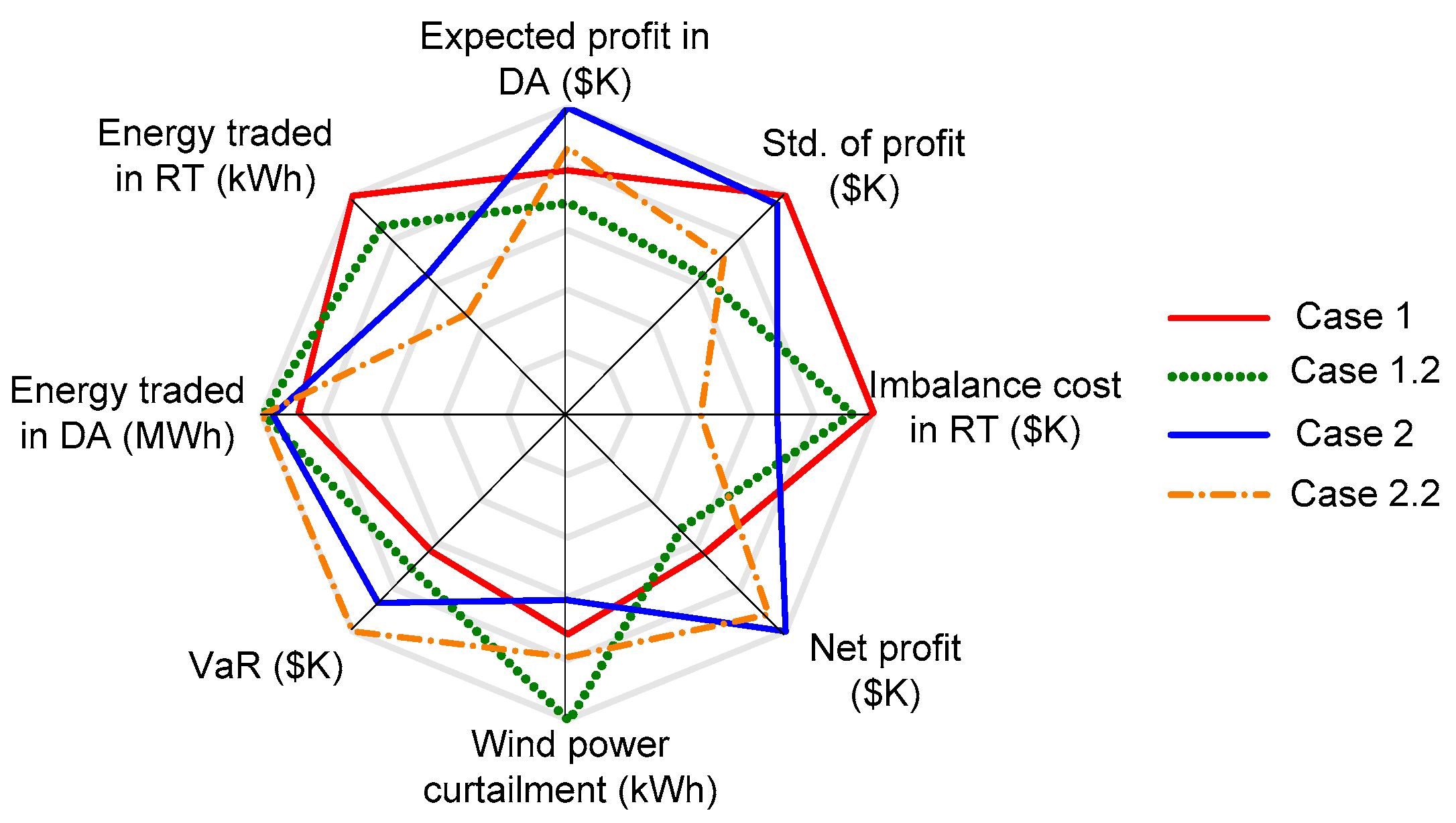
To demonstrate the impacts of different risk aversion levels, two more cases are added. Cases 1 and 2 are set with a higher weighting factor (), i.e., Case 1.2 and Case 2.2. Eight indicators are compared in the radar chart in Figure 8. Given the different scales, these indicators are presented in per unit (p.u.) based on the highest values in the four cases, i.e., $5823.30 = 1 p.u. expected profit; $1254.70 = 1 p.u. Std. of profit; $1593.50 = 1 p.u. imbalance cost; $4737.30 = 1 p.u. net profit; 1586.66 kWh = 1 p.u. wind power curtailment (WPC); $3982.30 = 1 p.u. VaR; 50.1463 MWh = 1 p.u. energy traded in DA; 1563.52 kWh = 1 p.u. energy traded in RT. As seen in Figure 8, for a higher weighting factor (more risk-averse), VPP becomes more conservative, thus more energy is traded in the DA market. In the meantime, more WP is curtailed, and VPP is more willing to buy electricity from the grid. Besides, a higher risk-aversion level leads to lower profit, lower Std. of profit, lower imbalance cost, and higher VaR. This reveals the trade-off between profit and risk, and the VPP should make trading decisions based on its risk preference. Moreover, for the uncoordinated strategies (Cases 1 and 1.2), DERs earn less profit but are exposed to higher risks. Therefore, the proposed model can effectively reduce the risks in relation to uncertainties.
The four cases are expanded to another four cases (Cases 1.3, 1.4, 2.3 and 2.4). This is done by increasing the uncertainties by 10% (i.e., the forecast errors of market price, load and wind power are increased by 10%). As seen in Table 3 and Table 4, the increased uncertainties result in higher imbalance costs and lower VaR for both operation strategies, which means higher risks. This implies that the VPP should use more sophisticated forecast techniques to hedge against the profit variation risks if increased uncertainties are expected (e.g., increased WP penetration in the future or increased market volatility). Moreover, in a more uncertain environment, WP is less efficiently used (e.g., WPC is increased from 956.36 kWh in Case 2 to 1456.39 kWh in Case 2.3) and more energy is traded in the RT market. It is worth mentioning that for a more conservative strategy (cases 2.2 and 2.4), the reduction in the net profit caused by the increased uncertainties is the least (the net profits are $4378.70 in Case 2.2 and $4270.10 in Case 2.4). Besides, the net profit in Case 2.4 ($4270.10) is higher than that in Case 2.3 ($3620.10). This proves that the profit reduction due to risk-aversion is minimized by adopting a more conservative integrated VPP operational strategy. In other words, the cost in relation to risk-aversion is effectively reduced.
To investigate the correlation between risk aversion and uncertainty parameters, four more cases are added by combing the low and high values of risk aversion and uncertainty parameters. Specifically, low and high risk aversion values are set at and , respectively, while low and high uncertainty values are set by decreasing and increasing the uncertainties by 10%. Case 2.5 is defined as a low risk aversion and low uncertainty case; Case 2.6 is defined as a low risk aversion and high uncertainty case; Case 2.7 is defined as a high risk aversion and low uncertainty case; and Case 2.8 is defined as a high risk aversion and high uncertainty case. The detailed results of cases 2.5–2.8 are given in Table 5. Based on the sensitivity analysis of risk aversion and uncertainty parameters, three findings can be identified in Table 5. First, a high risk aversion value results in marked reductions in expected profit, net profit, and energy trades in both DA and RT markets. This is because that if the VPP is more conservative, the VPP is more likely to use the DERs such as DG and BESS to meet the local demands, rather than trading energy in the markets. Second, a higher uncertainty value results in relatively smaller reductions in expected profit, net profit, and energy trades in the DA market. However, a higher uncertainty value results in marked increases in imbalance cost, wind power curtailment and energy trades in the RT market. This implies that the higher uncertainty value is likely to increase the inaccuracy of DA scheduling plans of the VPP, and hence more energy imbalance is traded. Third, the risk aversion and uncertainty parameters can influence each other. A positive correlation is observed between them, since both higher risk aversion and uncertainty parameters can result in reductions in the objective value (i.e., the net profit).
Furthermore, the proposed VPP scheduling approach is compared to another approach proposed in [16]. As seen in Table 6, the net profits of the VPP are $4737.30 and $4099.10 for the two approaches respectively. This proves that the proposed approach is superior in terms of optimality. More importantly, since the approach in [16] does not include any risk measure in the model, the risk of the VPP is marked higher (VaR for the approach in [16] is $2466.30 ). Note that a lower VaR means a higher risk of profit variability. Using the approach in [16], the VPP cannot understand the trade-off between risk and profit, and identifies a scheduling solution that entails a higher market risk. In addition, the renewable energy is not efficiently utilized, as the wind power curtailment is 1726.39 kWh for the approach in [16].
6. Conclusions
This paper presents an optimal scheduling model for a price-taker VPP participating in the DA and RT markets. In the DA market, the VPP maximizes the expected profit by determining the unit commitments and hourly scheduling of the DERs in its portfolio. To capture the risk of low profit scenarios, a risk factor based on the mean-variance Markowitz theory is incorporated into the objective function. In the RT market, the VPP minimizes the imbalance cost and wind power curtailment by adjusting the outputs of DERs on a five-minute basis. According to the simulation results in case studies, the VPP can help cost-efficient integration of DERs, and the integration is an effective risk-hedging mechanism. Specifically, the aggregated VPP scheduling approach can make more profit surplus, mitigate the impact of uncertainties, and reduce the cost of risk-aversion.
Acknowledgments
The work in this paper is supported by a China Southern Power Grid Research Grant WYKJ00000027, the National Natural Science Foundation of China (Key Programs 71331001 and 71420107027, and General Programs 71071025 and 71271033) and the Shenzhen Municipal Science and Technology Innovation Committee International R&D project (GJHZ20160301165723718).
Author Contributions
Jing Qiu did the simulation work and wrote the manuscript. Junhua Zhao, Dongxiao Wang, and Yu Zheng checked the model and proofread the manuscript.
Conflicts of Interest
The authors declare no conflict of interest.
Nomenclature
| Indices | |
| Bus | |
| Scenario | |
| Time | |
| Parameters | |
| Cost coefficients of interruptible load | |
| Cost coefficients of DG | |
| Cost coefficient of BESS lifetime degradation | |
| Rated energy of BESS | |
| Initial and final energy stored in BESS | |
| Relative differences between DA and RT electricity prices | |
| Investment cost of BESS | |
| Total lifecycle of BESS | |
| Minimum up and down time limits of DG | |
| Dis/charging loss factor and leakage loss factor of BESS | |
| Size of DE population | |
| Total scheduling intervals in RT | |
| Interconnection power exchange | |
| Retail price for customers | |
| Regulation up and down prices | |
| DA electricity price | |
| System reserve requirement | |
| Ramping up and down rates of DG | |
| Start-up and shut-down costs of DG | |
| Total scheduling intervals in DA | |
| Penalty price of wind power curtailment | |
| Cut-in, cut-out and rated wind speeds | |
| Weighting factor of risk | |
| Ratio of interruptible load | |
| Variables | |
| Operational cost of BESS | |
| Cost of DG | |
| Imbalance cost | |
| Cost of interruptible load | |
| Energy stored in BESS | |
| Fitness value of population | |
| Active and reactive power injection | |
| Active and reactive power demand | |
| Generated active and reactive power | |
| Active power output of DG | |
| Active power imbalance | |
| Forecasted power | |
| Scheduled power in DA | |
| Scheduled power in RT | |
| BESS power | |
| Wind active and reactive power | |
| Available wind power | |
| Active power loss | |
| Interruptible load power | |
| Complex power flow | |
| State of charge | |
| Voltage angle and amplitude | |
| Number of hours for which DG has been on or off | |
| Wind speed | |
| Individuals (candidate solutions) in the DE algorithm | |
| Commitment status of DG | |
| Start-up and shut-down binary decisions of DG | |
| Dis/charging binary decision of BESS | |
| Standard deviation of the objective | |
| Sets and others | |
| Set of wind power | |
| Set of BESS | |
| Set of DG | |
| Set of demand | |
| Set of scenarios | |
| Set of bus | |
| Objective of the DA dispatch model | |
| Objective of the RT dispatch model | |
| Upper and lower limits | |
| Expectation operator | |
| Probability operator | |
| Variables in RT | |
| Time factor | |
References
- Mashhour, E.; Moghaddas-Tafreshi, S.M. Bidding strategy of virtual power plant for participating in energy and spinning reserve markets—Part I: Problem formulation. IEEE Trans. Power Syst. 2011, 26, 949–956. [Google Scholar] [CrossRef]
- Asmus, P. Microgrids, virtual power plants and our distributed energy future. Electr. J. 2010, 23, 72–82. [Google Scholar] [CrossRef]
- Peik-Herfeh, M.; Seifi, H.; Sheikh-EI-Eslami, M.K. Decision making of a virtual power plant under uncertainties for bidding in a day-ahead market using point estimate method. Electr. Power Syst. Res. 2013, 44, 88–98. [Google Scholar] [CrossRef]
- Zhao, Q.; Shen, Y.; Li, M. Control and bidding strategy for virtual power plants with renewable generation and inelastic demand in electricity markets. IEEE Trans. Sustain. Energy 2016, 7, 562–575. [Google Scholar] [CrossRef]
- Pudjianto, D.; Ramsay, C.; Strbac, G. Virtual power plant and system integration of distributed energy resources. IET Renew. Power Gen. 2007, 1, 10–16. [Google Scholar] [CrossRef]
- Cao, C.; Xie, J.; Yue, D.; Huang, C.; Wang, J.; Xu, S.; Chen, X. Distributed economic dispatch of virtual power plant under a non-ideal communication work. Energies 2017, 10, 235. [Google Scholar] [CrossRef]
- Yang, H.; Yi, D.; Zhao, J.; Dong, Z.Y. Distributed optimal dispatch of virtual power plant via limited communication. IEEE Trans. Power Syst. 2013, 28, 3511–3512. [Google Scholar] [CrossRef]
- Pandzic, H.; Kuzle, I.; Capuder, T. Virtual power plant mid-term dispatch optimization. Appl. Energy 2013, 101, 134–141. [Google Scholar] [CrossRef]
- Dabbagh, S.R.; Sheihk-EI-Eslami, M.K. Risk-based profit allocation to ders integrated with a virtual power plant using cooperative game theory. Electr. Power Syst. Res. 2015, 121, 368–378. [Google Scholar] [CrossRef]
- Tajeddini, M.A.; Rahimi-Kian, A.; Soroudi, A. Risk averse optimal operation of a virtual power plant using two-stage stochastic programming. Energy 2014, 73, 958–967. [Google Scholar] [CrossRef]
- Liu, Y.; Xin, H.; Wang, Z.; Gan, D. Control of virtual power plant in microgrids: A coordinated approach based on photovoltaic systems and controllable loads. IET Gen. Transm. Dis. 2015, 9, 921–928. [Google Scholar] [CrossRef]
- Pandzic, H.; Morales, J.M.; Conejo, A.J.; Kuzle, I. Offering model for a virtual power plant based on stochastic programming. Appl. Energy 2013, 105, 282–292. [Google Scholar] [CrossRef]
- Kardakos, E.G.; Simoglou, C.K.; Bakirtzis, A.G. Optimal offering strategy of a virtual power plant: A stochastic bi-level approach. IEEE Trans. Smart Grid 2016, 7, 794–806. [Google Scholar] [CrossRef]
- Nezamabadi, H.; Nazar, M.S. Arbitrage strategy of virtual power plants in energy, spinning reserve and reactive power markets. IET Gen. Transm. Dis. 2016, 10, 750–763. [Google Scholar] [CrossRef]
- Karimyan, P.; Abedi, M.; Hosseinian, S.H.; Khatami, R. Stochastic approach to represent distributed energy resources in the form of a virtual power plant in energy and reserve markets. IET Gen. Transm. Dis. 2016, 10, 1792–1804. [Google Scholar] [CrossRef]
- Luo, F.J.; Dong, Z.Y.; Meng, K.; Qiu, J.; Yang, J.J.; Wong, K.P. Short-term operational planning framework for virtual power plants with high renewable penetrations. IET Renew. Power Gen. 2016, 10, 623–633. [Google Scholar] [CrossRef]
- Vasirani, M.; Kota, R.; Cavalcante, R.L.G.; Ossowski, S.; Jennings, N.R. An agent-based approach to virtual power plants of wind power generators and electric vehicles. IEEE Trans. Smart Grid 2013, 4, 1314–1322. [Google Scholar] [CrossRef]
- Markowitz, H.M. Portfolio Selection, Efficient Diversification of Investments; Yale University Press: New Haven, CT, USA, 1959. [Google Scholar]
- Dabbagh, S.R.; Sheihk-EI-Eslami, M.K. Risk assessment of virtual power plants offering in energy and reserve markets. IEEE Trans. Power Syst. 2016, 31, 3572–3582. [Google Scholar] [CrossRef]
- Skytte, K. The regulating power market on the nordic power exchange nord pool: An econometric analysis. Energy Econom. 1999, 21, 295–308. [Google Scholar] [CrossRef]
- Conejo, A.J.; Contreras, J.; Espinola, R.; Plazas, M.A. Forecasting electricity prices for a day-ahead pool-based electri energy market. Int. J. Forecast. 2005, 21, 435–462. [Google Scholar] [CrossRef]
- Conejo, A.J.; Carrion, M.; Morales, J.M. Decision Making under Uncertainty in Electricity Markets; Springer: New York, NY, USA, 2010. [Google Scholar]
- Zheng, Y.; Dong, Z.Y.; Luo, F.J.; Meng, K.; Qiu, J.; Wong, K.P. Optimal allocation of energy storage system for risk mitigation of discos with high renewable penetrations. IEEE Trans. Power Syst. 2014, 29, 212–220. [Google Scholar] [CrossRef]
- Hu, J. Coordinated control and fault protection investigation of a renewable energy integration facility with solar pvs and a micro-turbine. Energies 2017, 10, 423. [Google Scholar] [CrossRef]
- Atia, R.; Yamada, N. Distributed renewable generation and storage system sizing based on smart dispatch of microgrids. Energies 2016, 9, 176. [Google Scholar] [CrossRef]
- Huang, J.; Xue, Y.; Dong, Z.Y.; Wong, K.P. An efficient probabilistic assessment method for electricity market risk management. IEEE Trans. Power Syst. 2012, 27, 1485–1493. [Google Scholar] [CrossRef]
- Leong, K.; Siddiqi, R. Value at risk for power markets. In Energy Risk Management; McGraw-Hill: New York, NY, USA, 1998; pp. 157–178. [Google Scholar]
- Birge, J.R.; Louveaux, F. Introduction to Stochastic Programming; Springer: New York, NY, USA, 1997. [Google Scholar]
- Zhang, H.; Vittal, V.; Heydt, G.T.; Quintero, J. A mixed-integer linear programming approach for multi-stage security-constrained transmission expansion planning. IEEE Trans Power Syst. 2012, 27, 1125–1133. [Google Scholar] [CrossRef]
- Yang, G.Y.; Dong, Z.Y.; Wong, K.P. A modified differential evolution algorithm with fitness sharing for power system planning. IEEE Trans. Power Syst. 2008, 23, 514–522. [Google Scholar] [CrossRef]
- Zhao, C.; Wang, J.; Watson, J.; Guan, Y. Multi-stage robust unit commitment considering wind and demand response uncertainties. IEEE Trans. Smart Grid 2013, 28, 2708–2717. [Google Scholar] [CrossRef]
- Moghaddas-Tafreshi, S.M.; Mashhour, E. Distributed generation modeling for power flow studies and a three-phase unbalanced power flow solution for radial distribution systems considering distributed generation. Electr. Power Syst. Res. 2009, 79, 680–686. [Google Scholar] [CrossRef]
- Zhang, R.; Dong, Z.Y.; Xu, Y.; Wong, K.P.; Lai, M. Hybrid computation of corrective security-constrained optimal power flow problems. IET Gen. Trans. Dist. 2014, 8, 995–1006. [Google Scholar] [CrossRef]
- Nord Pool Historical Market Data. Available online: http://www.nordpoolspot.com/historical-market-data/ (accessed on 5 March 2017).
- Ghofrani, M.; Arabali, A.; Etezadi-Amoli, M.; Fadali, M.S. Energy storage application for performance enhancement of wind integration. IEEE Trans. Power Syst. 2013, 28, 4803–4811. [Google Scholar] [CrossRef]
Figure 1.
Concept of virtual power plant (VPP) and its components.
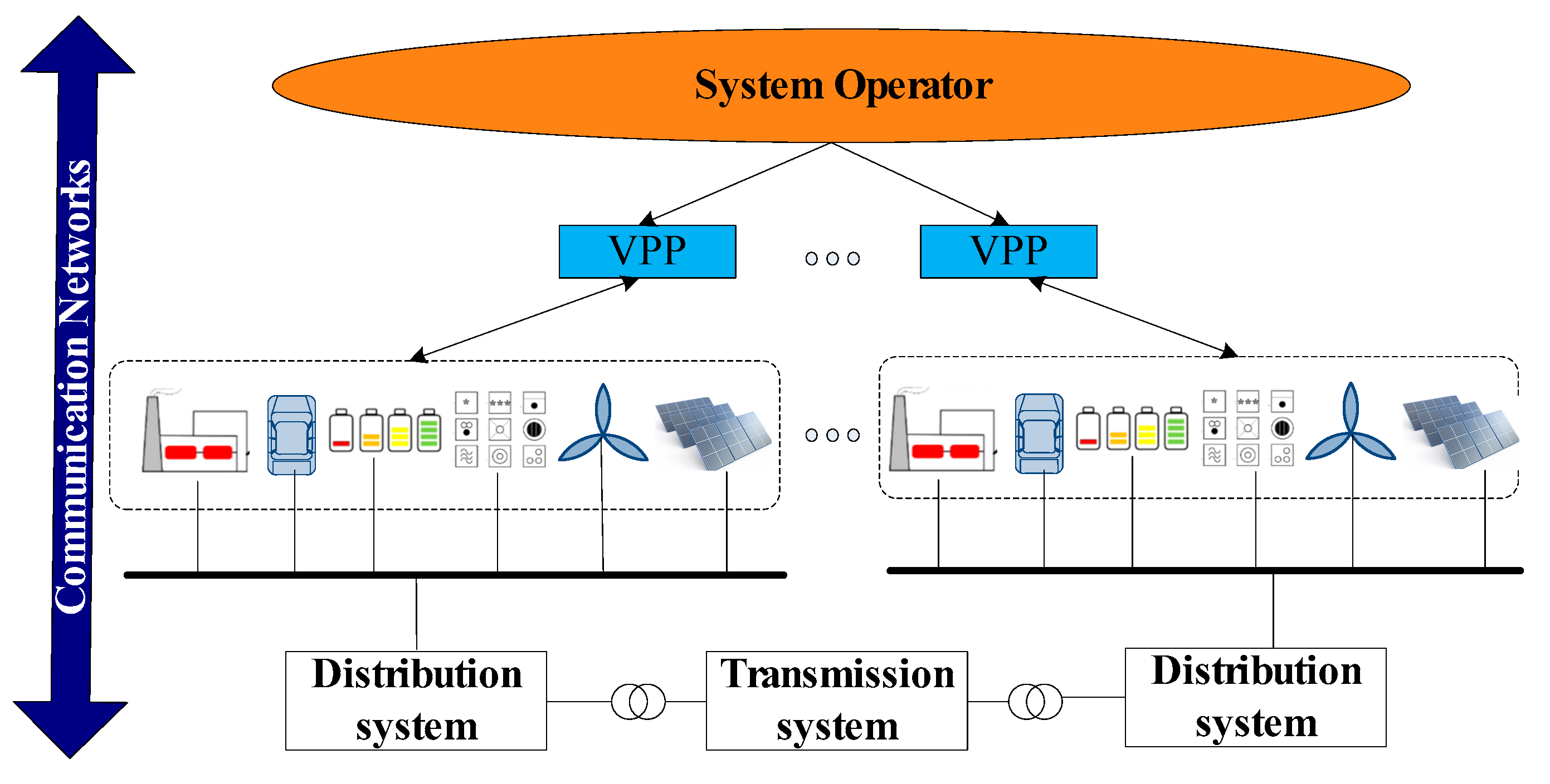
Figure 2.
Flow chart of the applied solution algorithm.
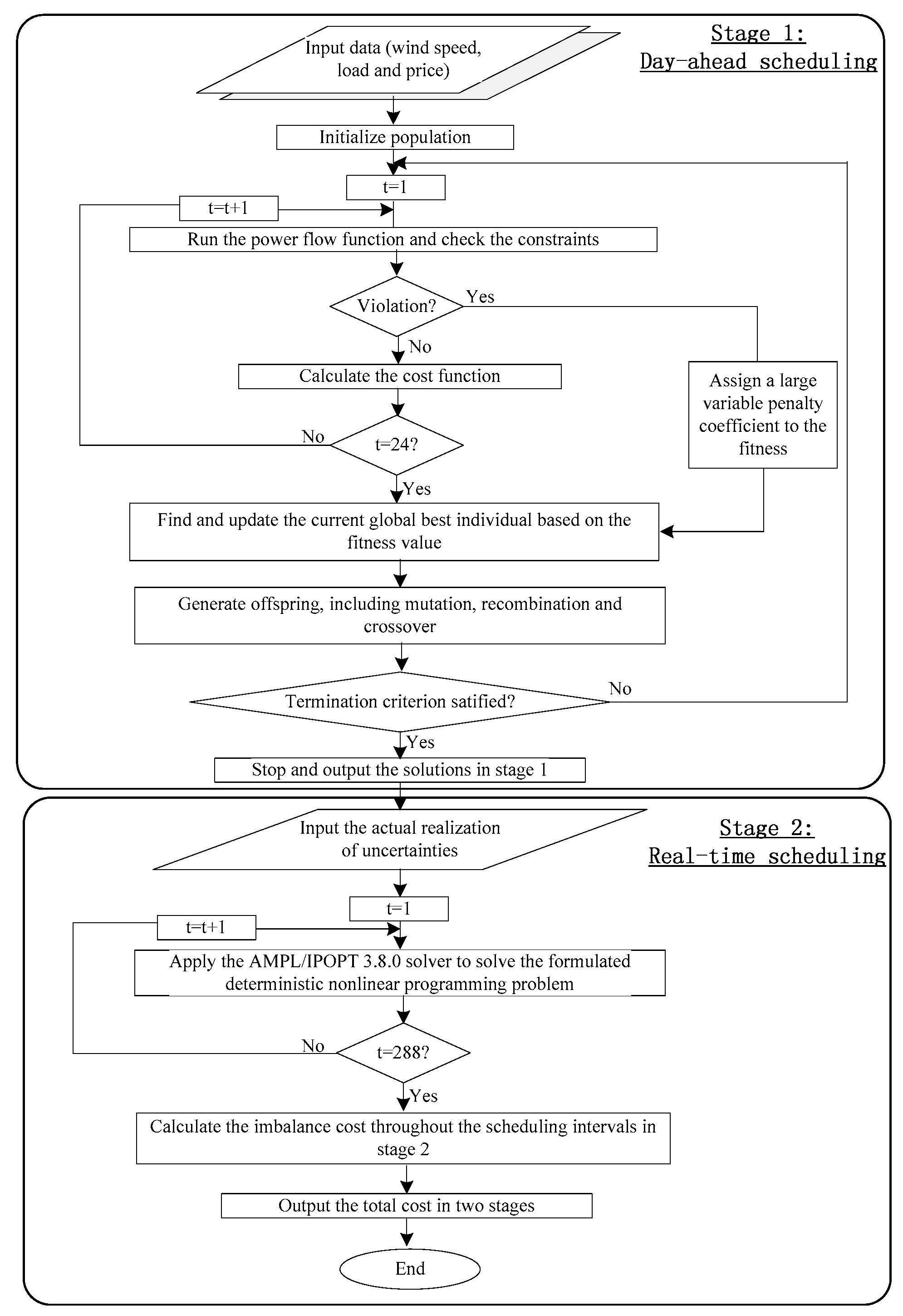
Figure 3.
One-line diagram of the 12-bus VPP system.

Figure 4.
Distributions of the expected profits in the DA market for Cases 1 and 2.
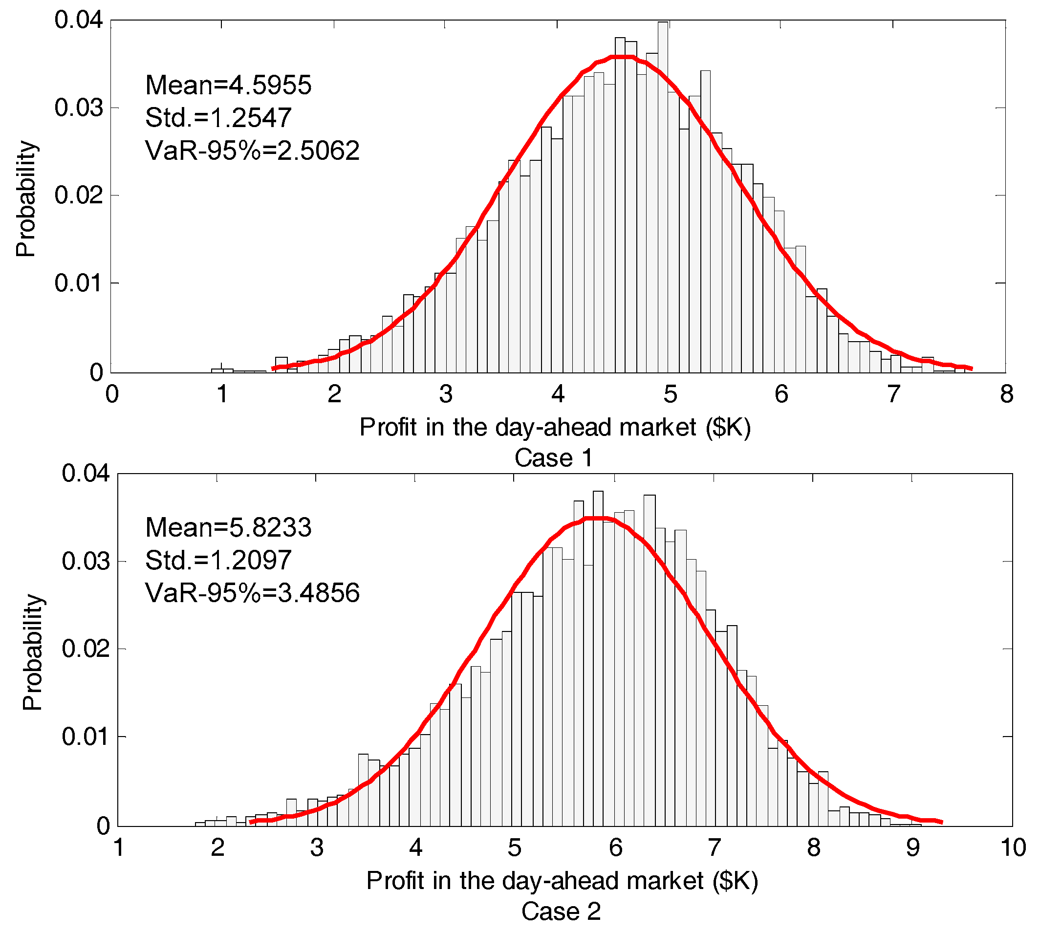
Figure 5.
Computation performances for Cases 1 and 2.

Figure 6.
Energy in BESS and dis/charged power in two markets for Cases 1 and 2.
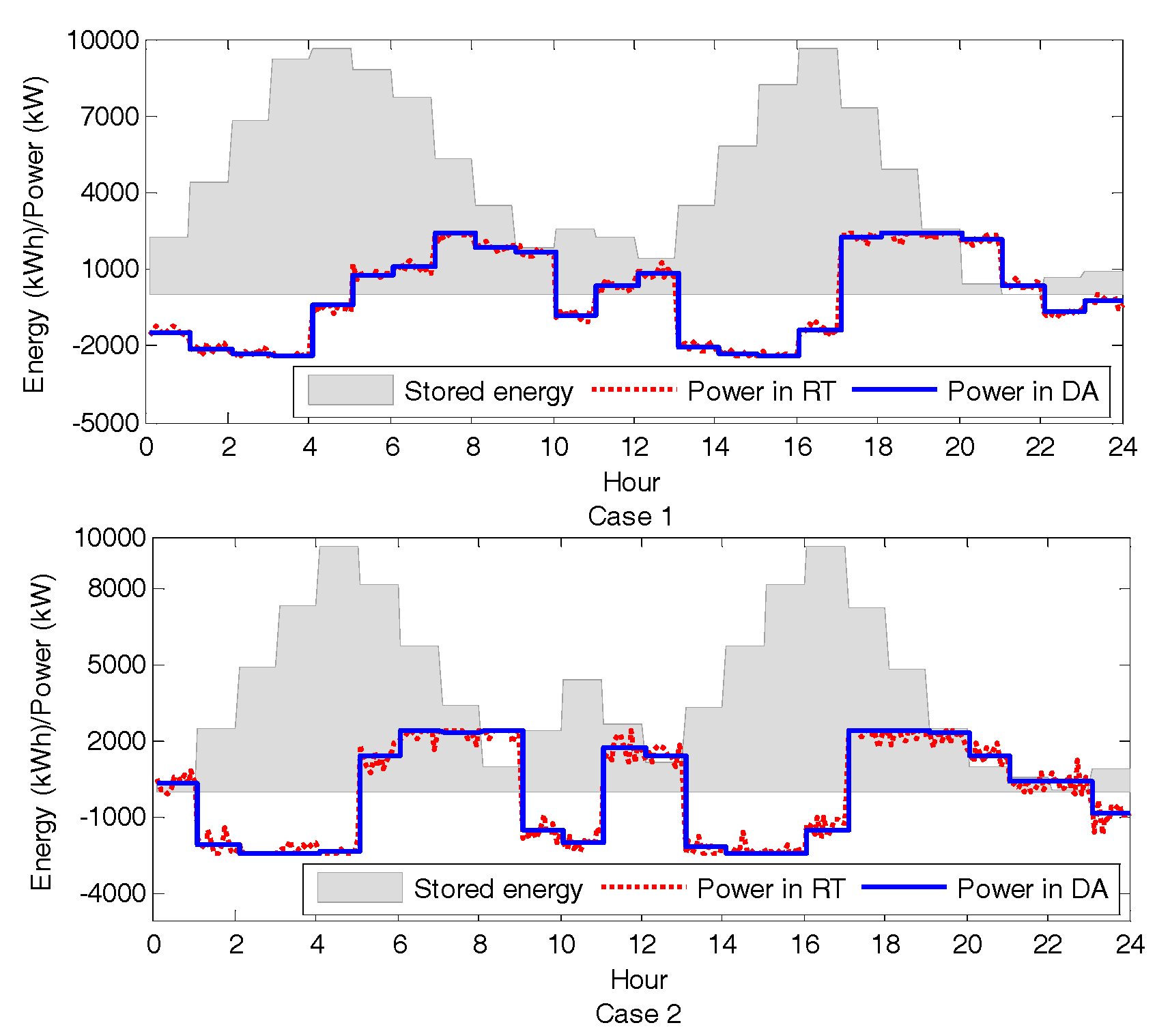
Figure 7.
Power production and demand and energy traded in the DA market.

Figure 8.
Performance evaluation of different cases.


Table 1.
Profits and costs for VPP components in Case 1.
| Cost/Profit | DG | BESS | WP | IL | Total |
|---|---|---|---|---|---|
| Expected profit ($) | 369.40 | 2089.50 | 1679.80 | 456.80 | 4595.50 |
| Imbalance cost ($) | 32.80 | 8.70 | 1426.80 | 125.20 | 1593.50 |
| Net profit ($) | 336.60 | 2080.80 | 253.00 | 331.60 | 3002.00 |
Table 2.
Profits and costs for VPP components in Case 2
| Cost/Profit | DG | BESS | WP | IL | Total |
|---|---|---|---|---|---|
| Expected profit ($) | 1201.20 | 2178.90 | 1856.90 | 586.30 | 5823.30 |
| Imbalance cost ($) | 31.50 | 55.00 | 815.40 | 184.10 | 1086.00 |
| Net profit ($) | 1169.70 | 2123.90 | 1041.50 | 402.20 | 4737.30 |
Table 3.
Sensitivity analysis for uncoordinated operation.
| # | Case 1 | Case 1.3 | Case 1.2 | Case 1.4 |
|---|---|---|---|---|
| Expected profit ($) | 4595.50 | 4265.20 | 3985.60 | 3968.50 |
| Std. ($) | 1254.70 | 1365.20 | 786.20 | 1058.90 |
| Imbalance cost ($) | 1593.50 | 1896.20 | 1486.30 | 1898.20 |
| Net profit ($) | 3002.00 | 2369.00 | 2499.30 | 2070.30 |
| WPC (kWh) | 1132.65 | 1685.35 | 1586.66 | 1785.85 |
| VaR ($) | 2506.20 | 2235.50 | 2863.30 | 2248.50 |
| Energy traded DA (MWh) | 43.98 | 44.26 | 50.14 | 51.26 |
| Energy traded RT (kWh) | 1563.50 | 1653.38 | 1354.61 | 1458.69 |
Table 4.
Sensitivity analysis for integrated VPP operation.
| # | Case 2 | Case 2.3 | Case 2.2 | Case 2.4 |
|---|---|---|---|---|
| Expected profit ($) | 5823.30 | 4985.30 | 5068.00 | 5012.50 |
| Std. ($) | 1209.70 | 1458.60 | 893.50 | 1126.60 |
| Imbalance cost ($) | 1086.00 | 1365.20 | 689.30 | 742.50 |
| Net profit ($) | 4737.30 | 3620.10 | 4378.70 | 4270.10 |
| WPC (kWh) | 956.36 | 1456.39 | 1263.28 | 1268.92 |
| VaR ($) | 3485.60 | 2866.30 | 3982.30 | 3569.80 |
| Energy traded DA (MWh) | 48.25 | 48.66 | 50.12 | 50.98 |
| Energy traded RT (kWh) | 1012.35 | 1456.36 | 725.36 | 996.48 |
Table 5.
Sensitivity analysis for risk aversion and uncertainty parameters.
| # | Case 2.5 | Case 2.6 | Case 2.7 | Case 2.8 |
|---|---|---|---|---|
| Expected profit ($) | 6525.60 | 6023.30 | 4612.70 | 4472.10 |
| Std. ($) | 1337.40 | 1886.30 | 986.10 | 1209.70 |
| Imbalance cost ($) | 1093.30 | 1532.10 | 832.30 | 1224.50 |
| Net profit ($) | 5432.30 | 4491.20 | 3780.40 | 3247.60 |
| WPC (kWh) | 655.18 | 1308.62 | 652.32 | 756.48 |
| VaR ($) | 4002.40 | 3026.20 | 4523.90 | 3369.20 |
| Energy traded DA (MWh) | 55.26 | 51.25 | 42.36 | 41.23 |
| Energy traded RT (kWh) | 701.92 | 1512.35 | 422.18 | 1217.36 |
Table 6.
Result comparison to an approach in the literature.
| # | Proposed Approach | Approach in [16] |
|---|---|---|
| Expected profit ($) | 5823.30 | 5172.70 |
| Std. ($) | 1209.70 | 1463.30 |
| Imbalance cost ($) | 1086.00 | 1073.60 |
| Net profit ($) | 4737.30 | 4099.10 |
| WPC (kWh) | 956.36 | 1726.39 |
| VaR ($) | 3485.60 | 2466.30 |
| Energy traded DA (MWh) | 48.25 | 45.18 |
| Energy traded RT (kWh) | 1012.35 | 1004.88 |
© 2017 by the authors. Licensee MDPI, Basel, Switzerland. This article is an open access article distributed under the terms and conditions of the Creative Commons Attribution (CC BY) license (http://creativecommons.org/licenses/by/4.0/).
Share and Cite
MDPI and ACS Style
Qiu, J.; Zhao, J.; Wang, D.; Zheng, Y. Two-Stage Coordinated Operational Strategy for Distributed Energy Resources Considering Wind Power Curtailment Penalty Cost. Energies 2017, 10, 965. https://doi.org/10.3390/en10070965
AMA Style
Qiu J, Zhao J, Wang D, Zheng Y. Two-Stage Coordinated Operational Strategy for Distributed Energy Resources Considering Wind Power Curtailment Penalty Cost. Energies. 2017; 10(7):965. https://doi.org/10.3390/en10070965
Chicago/Turabian StyleQiu, Jing, Junhua Zhao, Dongxiao Wang, and Yu Zheng. 2017. "Two-Stage Coordinated Operational Strategy for Distributed Energy Resources Considering Wind Power Curtailment Penalty Cost" Energies 10, no. 7: 965. https://doi.org/10.3390/en10070965
Note that from the first issue of 2016, this journal uses article numbers instead of page numbers. See further details here.