
An Innovative Hybrid Model Based on Data Pre-Processing and Modified Optimization Algorithm and Its Application in Wind Speed Forecasting


1
School of Statistics, Dongbei University of Finance and Economics, Dalian 116025, China
2
Key Laboratory of Arid Climatic Change and Reducing Disaster of Gansu Province, College of Atmospheric Sciences, Lanzhou University, Lanzhou 730000, China
*
Author to whom correspondence should be addressed.
Energies 2017, 10(7), 954; https://doi.org/10.3390/en10070954
Submission received: 22 June 2017
/
Revised: 4 July 2017
/
Accepted: 4 July 2017
/
Published: 9 July 2017
(This article belongs to the Special Issue Hybrid Advanced Optimization Methods with Evolutionary Computation Techniques in Energy Forecasting)
Abstract
:Wind speed forecasting has an unsuperseded function in the high-efficiency operation of wind farms, and is significant in wind-related engineering studies. Back-propagation (BP) algorithms have been comprehensively employed to forecast time series that are nonlinear, irregular, and unstable. However, the single model usually overlooks the importance of data pre-processing and parameter optimization of the model, which results in weak forecasting performance. In this paper, a more precise and robust model that combines data pre-processing, BP neural network, and a modified artificial intelligence optimization algorithm was proposed, which succeeded in avoiding the limitations of the individual algorithm. The novel model not only improves the forecasting accuracy but also retains the advantages of the firefly algorithm (FA) and overcomes the disadvantage of the FA while optimizing in the later stage. To verify the forecasting performance of the presented hybrid model, 10-min wind speed data from Penglai city, Shandong province, China, were analyzed in this study. The simulations revealed that the proposed hybrid model significantly outperforms other single metaheuristics.
1. Introduction
Wind power is one of the most significant recycled energy resources presently being applied [1]. Recently, due to the pollution of the global environment, recyclable energy [2] and non-polluting sources such as wind energy have been gaining extensive attention [3]. Wind energy, which is one of the most promising and active recyclable sources, is providing an increasingly strong supplement to traditional energy sources [4]. When it comes to the accurate forecasting of wind speed and its wide use in wind power, we encounter great challenges, because the wind is a periodical phenomenon [5] with a nonlinear, anomalistic, and stochastic nature. Wind speed forecasting is applied in several domains, for instance, target tracking, shipping, weather forecasting, agricultural production, and electric load forecasting. To dispatch wind energy before wind power grid integration, it is very important for a wind farm operator to accurately determine the wind speed. This is because the local wind speed is always the foremost factor affecting wind power generation, and can be used for wind turbine selection and for wind farm layout [6]. In addition, wind speed can enhance the power system’s schedule and strengthen resource configuration, promoting the reliability of the power grid. Predictions made with higher precision can allow power system operators to dispatch power efficiently in order to properly meet the demands of consumers [7].
Given a more precise wind speed value, the power operator is able to forecast power delivery. This is extremely helpful for power systems in terms of optimizing storage capacity, making sensible and proper programs, and dispatching electric energy well. Because of the wind’s irregularity and complex fluctuations, variations in wind speed forecasting may result in quick changes in the prediction results of wind power. This feature indicates that accurate wind speed forecasting is highly important. The wind speed forecast plays a vital role in utilizing wind power appropriately and efficiently. Various methods have been proposed to promote the accuracy of wind speed prediction. Three of the most extensively used methods are the physical forecasting method, the conventional statistical method, and the artificial intelligence method. Given a series of meteorological parameters, the physical forecasting method uses physical variables to derive a time series forecast. Therefore, higher prediction accuracy can be obtained using this method [8]. However, their extremely intricate computations always lead to it being largely a waste of time. Numerical weather forecasting is one of the most widely used physical forecasting methods, consisting of a computer program that aims to solve questions through meteorological data processing and describe how the atmosphere changes as time goes on [9]. In addition, the traditional approaches include the regression analysis method, the auto-regressive integrated moving average (ARIMA) [10] model, the non-parametric estimation method, exponential smoothing [11], the state-space model [12], Box-Jenkins models [13], the spatial correlation model, and the difference method. Furthermore, support vector machines (SVMs) [14] such as non-neural networks are also frequently applied in wind speed forecasting.
Among the above methods, artificial neural networks (ANNs) have been frequently and widely applied. By imitating the human brain in handling information with a sequence of neurons, ANNs obtain a distinguished capacity for mapping, and their complex and highly nonlinear input and output modes with making nothing of the type of real model can establish some simple models and compose different networks depending on different connections. Therefore, ANNs demonstrate the following advantages: high adaptability, excellent ability to learn using cases, and ability to summarize. It is well known that the multi-layered perceptron (MLP) is one of the most broadly used ANN methods. The vast majority of available methods that can be used to train ANNs pay close attention only to the alteration of connection weights in a certain topology, which usually leads to defective results.
MLPs are prosperously applied in many fields, such as pattern classification [15], digit recognition [16], image processing, coal price prediction [17], function approximation, measurement of object shape [18], and adaptation control. The back-propagation (BP) algorithm [19] performs most effectively of all training algorithms for MLP methods. The selection of a suitable structure for the forecasting question and the alteration of connection weights of the network constitute the two parts of training MLPs for the problem. Several studies have been successfully used to solve these issues.
A great deal of research has been conducted to precisely forecast the wind energy and the local value of wind speed. Wind power and speed forecast is a fundamental problem for wind farm operation, best power flow between the electric system and wind power plant, market price, electric power system dispatching, and wind power resource reserve, and storage programming and dispatching. Over the last few decades, the ANN [20,21] has been the superior model, and has frequently been applied to forecast time series.
The ANN is a pragmatic calculation method, similar to the human biological neuron. Various improvable neural networks exist, of which the following two are the most frequently employed: feed forward neural networks and feedback neural networks. Feed forward neural networks have no feedback. On the contrary, feedback neural networks possess a feedback. Back-propagation (BP) neural networks, perceptrons, and radial basis function (RBF) networks play an important role in feed forward networks. Recurrent Neural Networks (RNNs) [22] and pulsed neural networks are two important models of feedback networks. The feedback networks mainly consist of RNN and spiking neural networks [23]. In this paper, we pay more attention to feed forward neural networks [24].
The BP algorithm has various significant advantages; for example, it can help to roughly estimate a great many functions, it is relatively simple to implement, and it can be used as a reference method. In addition, its most effective characteristic is that the momentum parameter and the learning rate factor can be altered, thereby enhancing the innovation speed of the traditional BP algorithm.
To gain good forecasting accuracy and low deviation, many studies [25,26,27,28,29,30,31,32] have been conducted to determine the optimal weights of neural networks. However, an original hybrid model system—a traditional hybrid method based on the rapid searching theory developed by Xiao et al. [33]—has been put into use. An extensive study was conducted by Xiao et al. [33] using four test functions to evaluate the optimization algorithm’s capacity for development, searching, avoiding partial optima, and convergence velocity, and the results of this experiment demonstrated that the modified method is more sufficient and excellent than the original algorithm. In recent years, a number of developmental optimization algorithms have been applied to help confirm the threshold values of a prediction method. Particle swarm optimization (PSO) was applied by Liu et al. [25] to optimize the parameters of the prediction technique for short-term electric load prediction in micro-grids. Wang et al. [26] employed a modified PSO to optimize the weight distribution of their proposed combined model developed for electric load prediction. The cuckoo search (CS) algorithm [27,28,29] was applied to determine the parameters of the proposed model for electric load forecasting. Wang et al. [30] modified the CS method to optimize the parameters of multi-step-ahead wind speed forecasting models. Xiao et al. [31] applied the genetic algorithm (GA) to optimize the parameters of the proposed model. In the present paper, a highly valid optimization method, the Broyden-Fletcher-Goldfarb-Shanno-Firefly Algorithm (BFGS-FA), is used to determine the parameters of the proposed hybrid model.
Recently, numerous continuous and novel improvements have been made to promote the effectiveness of the FA for optimizing neural networks, including the binary, Gaussian, firefly, high-dimensional firefly, Lévy flight, simultaneous firefly, and chaos-based FA [34,35]. Though most of these improvements to the FA enhance its performance successfully, few of them have been introduced to optimize the parameters of hybrid models. This paper intends not only to enhance the research and development abilities of the FA, but also to minimize the drawback of the partial optima seeking capacity, which appeared in the CS algorithm. On the basis of the BFGS quasi-Newton method, an original improvement of the FA was proposed to enhance the diversity of species of fireflies. Obviously, increasing the convergence standard may result in individual fireflies likely being caught in partial optima; however, it decreased when this optimized algorithm was used. Of course, the decomposition of the original wind sequence is a significant process for data filtering. This can always effectively promote the prediction accuracy of the model to obtain better forecast results [36]. Important techniques, such as empirical mode decomposition (EMD) [37], wavelet decomposition (WD) [38], and singular spectrum analysis (SSA) are often applied to remove the noise series. However, the wavelet de-noising algorithm is sensitive to the determination of the threshold, and the EMD may lead to mode confusion [39], which may result in a badly decomposed performance. In addition, SSA has many advantages, and overcomes the disadvantages of EMD and WD in terms of decomposition. Moreover, we analyzed some articles in the literature [40,41,42,43,44] that deal with wind forecasting by applying neural networks, and that are in line with the theme of the present paper. From these studies, we found that some data preprocessing or optimization algorithms are insufficient, and the details are listed in Table 1. Therefore, based on the discussed limitations, this manuscript proposes a characteristic hybrid model that unites the BP algorithm, SSA theory, and BFGS-FA. Ten-minute wind speed values collected from Penglai city, Shandong province, China, were applied to verify the unique hybrid model. The results of tests and practices in this study indicate that the hybrid model considerably outperformed the other three models. This demonstrates that the hybrid method could be applied to calculate wind speeds, which would be beneficial for enabling wind power system to make optimal decisions, such as providing better sites of wind power, taking early measures to reduce losses that can be caused due to bad weather, reducing production costs, and minimizing energy consumption (coal, etc.). This model is also useful for helping wind power companies to make correct decisions in real life. Thus, the hybrid forecasting method with high accuracy represents a model that will have potential application in the near future. Furthermore, the practical hybrid model can also be applied to other forecasting domains, such as target tracking, stock index forecasting, environment forecasting, shipping, weather forecasting, agricultural production, and electric load forecasting.
The primary contributions and novelties of this manuscript are listed as follows: (a) The BFGS-FA method, back propagation neural network (BPNN), and the concept of the de-noising algorithm were combined to form two new models: singular spectrum analysis-back propagation (SSA-BP), and singular spectrum analysis-Broyden-Fletcher-Goldfarb-Shanno-Firefly Algorithm-back propagation (SSA-BFGS-FA-BP). (b) This paper evaluates the developed models on the basis of two aspects: forecasting accuracy and stability. The results indicate that BFGS-FA-BP is a better model when considering accuracy only, but the hybrid SSA-BFGS-FA-BP is a better model overall: even with the low cost of calculation, the accuracy remained high. (c) The novel combined BFGS-FA algorithm successfully avoids the shortcomings of FA while optimizing, during the later period, the low velocity and the poor convergence performance. (d) The proposed hybrid approach integrates the advantages of other individual models. (e) A time sequence pre-processing method was applied to de-noise the raw data successfully.
The remainder of this paper is designed as follows. Section 2 presents the single prediction method developed according to the BPNN and the hybrid forecasting method theory. This section also describes the optimization algorithms BFGS, FA, and their combination BFGS-FA, which are applied to confirm the parameters of the hybrid forecasting model. SSA theory and the Diebold-Mariano (DM) test, which can help to determine the forecasting effectiveness of the developed hybrid method, are introduced at the end of Section 2. In Section 3, the wind speed time sequences collected from three separate sites are used to test the proposed hybrid model. Subsequently, the wind resources and the evaluation criteria of the forecasting model are described. In Section 4, we give a discussion about this study. In the end, Section 5 concludes this paper.
2. Methodology
Since McCulloch and Pitts [45] proposed the neural network mathematical model in 1943, ANNs have been applied in numerous fields, including signal processing, market analysis and forecasting, pattern recognition, and automatic control. In this part, separate theories of this innovative hybrid model will be introduced in detail.
2.1. BP Algorithm
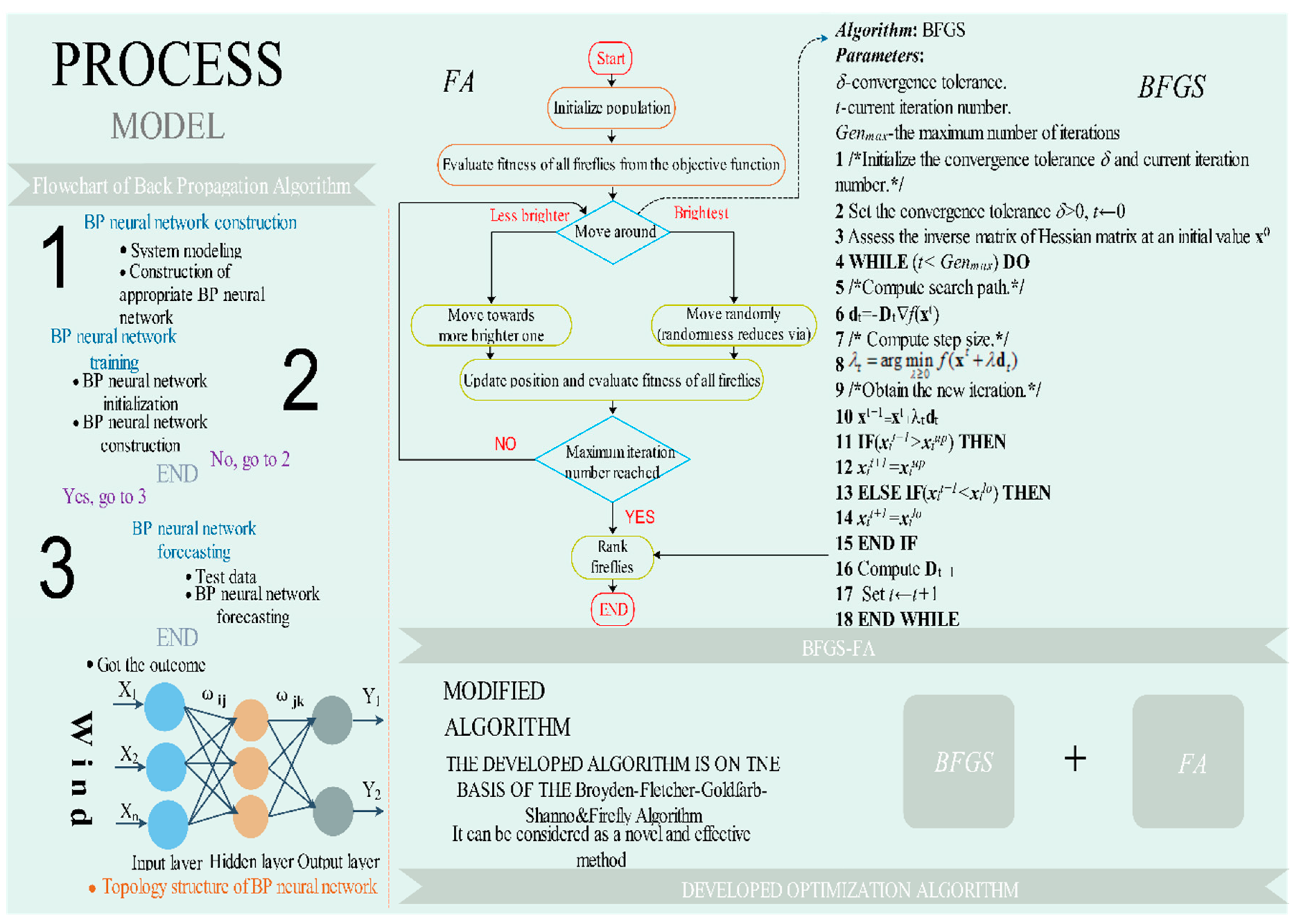
In mathematically simulating the human brain system, the BP algorithm benefits from its underlying processes, fuzzy information processing, and chaotic performance. On account of the error BP algorithm and the multilayer neural network, the BP neural network performs excellently in training ANNs. An input layer, one or more hidden layers, and an output layer constitute a representative BP network. The BP algorithm is always applied to adjust the thresholds, in which the errors from the output are propagated back into the network, transforming the thresholds as it goes, in order to keep the error [46] from emerging again. Its topology and flow structure are as follows:
The main procedures of the BP algorithm can be generalized as follows:
Step 1. We obtain the wind speed time sequence and corresponding parameter values from the wind power plant. The inputs have exhaustive information on historical values. The input value is often affected by the site, surrounding temperature, air pressure, time, and even the collectors. Our primary task is to make full use of four different parameters collected from the wind power plant.
Step 2. We transform the original value into the requested form (0 to 1). The normalization method is summarized as follows:
Step 3. We build the BP algorithm and set its parameters, which include the number of neurons in the input layer, hidden layer, and output layer; the learning rate; the maximum training times; and training requirement accuracy. The training can be summarized as learning from the historical values to discover the implied information among the previous time series data, which can be applied to forecast the future wind speed.
Step 4. We use the testing set to assess the effectiveness of the trained BP network.
Step 5. In the end, the future wind speed value (output) is forecast by the neural network.
2.2. Broyden-Fletcher-Goldfarb-Shanno
The BFGS [47] algorithm is an excellent method, and one of the most useful nonlinear quasi-Newton procedures.
Definition 1.
Let xt be the consequence at the representative iteration t and be a recursive function in which λt is the step size. The hunting path is , in which Dt is an positive certain symmetric matrix as a proximity of the inverse matrix of the real Hessian matrix at xt.
Definition 2.
The new path of BFGS can be designed as follows:
where
In addition, the primary BFGS algorithm is generalized in Appendix A.
2.3. Firefly Algorithm
The FA was first proposed by Xin-She Yang in 2008 [48]. The FA was inspired by the flashing nature of fireflies [49,50]. The firefly will be shining while flying, which can be regarded as a signal to attract other companions. The method has three regulations:
- (1)
- All fireflies are unisexual; in addition, any firefly can be attracted by others.
- (2)
- Attraction is directly proportional to their brightness; that is, for any two fireflies, the less bright one will be attracted by the brighter one, and will move towards it; the brightness will decrease as the distance between them increases.
- (3)
- If there are no brighter fireflies around a known firefly, it will fly at random. The brightness of the firefly must be tightly related to the objective function.
The experimental set points of the FA are described in Table 3.
The FA is a developed computational method that is also used to optimize controller parameters. Each firefly in the FA indicates a solution to the problem, which is defined on the basis of position. In a d-dimensional vector space, the present location of the ith firefly is acquired by . The random positions of m fireflies are initialized within the specified range. The position updating equation for the ith firefly, which is attracted to move to a brighter firefly j, is given as follows:
In addition, the position updating equation for the brightest firefly is given as follows:
where the first terms xi(t) and xbesti(t) of Equations (4) and (5) are the current positions of a less bright firefly and the brightest firefly, respectively. The second term in Equation (4) is the firefly’s attraction to light intensity. β0 is the original attraction at r = 0, γ is the absorption parameter in the range [0, 1], and is the distance between any two fireflies i and j, at position and , respectively, and can be formulated as a Cartesian or Euclidean distance as follows:
where and are the position vectors for fireflies i and j, respectively, with representing the position value for the dimension, and the third term in Equation (4) and the second term in Equation (5) are used to reduce the randomness; that is, the movement of the fireflies is gradually reduced according to α = α0δt, where α0 is in the range [0, 1]. δ is the random reduction parameter where 0 < δ <1, and t is the iteration number. Every new position must be evaluated by a fitness function, which is assumed to be integral square error. The flow chart of the FA is presented in Figure 1, and the original FA algorithm is summarized in Appendix B.
2.4. BFGS-FA
FA possesses good global optimization and development capacities; however, it will usually be manifest a low velocity and poor convergence performance while optimizing in the later stage. Therefore, as shown in Figure 1, the BFGS is applied while FA renews the answers after a generation to search for a sub-optimization solution, which can be used to promote the partial optimization capacity and the rate of partial convergence of the total method. The primary method of BFGS-FA is generalized in Appendix C.
2.5. Singular Spectrum Analysis (SSA)
In America and England, SSA has been exploited separately based on singular spectrum analysis, whereas in Russia, it was proposed under the name Caterpillar-SSA [51]. SSA possesses the superiority of statistics and probability theory; meanwhile, it assimilates the knowledge of power systems and signal processing ideas.
Suppose that is a time sequence with T elements. The SSA method contains two parts: decomposition and reconstruction [52,53].
2.5.1. Decomposition
In decomposition, an observed unidimensional time series data is converted into its trajectory matrix. Subsequently, and its corresponding singular value decomposition (SVD) are computed. This can be divided into two steps: embedding and SVD.
Step 1. The primary aim of this step is to propose the concept of the trajectory matrix or deferred edition of the initial time sequence y. The main purpose of this step is to propose the concept of a trajectory matrix or a hysteretic version of the initial time sequence y. The resulting matrix has a window width W (W ≤ T/2), which is usually determined by the operator. Suppose that P = T − W + 1, the trajectory matrix is denoted as follows:
In fact, this trajectory matrix is a Hankel matrix; that is, all the elements of the diagonal i + j = const are equal [54].
Step 2. We obtain the covariance matrix from X. processed by the SVD will result in a group of L eigenvalues and their corresponding eigenvectors U1, U2, …, UL, which are often defined by empirical orthogonal functions. Therefore, the SVD of the trajectory matrix could be denoted as , where , d is the rank of (the total amount of non-zero characteristic values) and V1, V2,…,Vd are the corresponding principal components, which are denoted by . The set (, Ui, Vi) is the ith eigenvalue of the matrix X. Suppose that , then —the ratio of the variance of X—which is defined by Ei:E1, has the highest contribution [55], and Ed has the minimum contribution. The SVD will consume more elapsed time if the length of the time sequence is long enough (i.e., T > 1000).
2.5.2. Reconstruction
We compute and its SVD to obtain its L eigenvalues: and its corresponding eigenvectors. Each signal, as represented by the eigenvalue, is analyzed and assembled to reconstruct the new time series. This section can be resolved into two steps: grouping and averaging.
Step 1. Here, the designer chooses r out of d eigenvalues. Define to be a set of r chosen eigenvalues and , in which is connected to the “information” of y; nevertheless, the remaining (d–r) eigenvalues, which are not selected, represent the error term ε.
Step 2. The set of r elements chosen from the foregoing section is then applied to regroup the definitive elements of the time sequence. The fundamental concept is to convert each of the terms into the reconstructed data time series by using the Hankelization process H(Z) or diagonal averaging: assume Zij is an element of the ordinary matrix Z, then the kth term of the rebuilt time sequence could be acquired by averaging Zij, on the precondition of i + j = k + 1. Obviously, H(Z) is a time sequence with T elements rebuilt by matrix Z.
After averaging, we can obtain the approximation of y, which is the regrouped time series, and is given as follows:
From the whole time series, a singular eigenvalue will be reconstructed as suggested by Alexandrov and Golyandina. This indicates that SSA is not an awkward algorithm, and is therefore strong to abnormal values.
In addition, as shown in Figure 2, the original wind speed preprocessed by SSA is forecast by the BP algorithm, and its parameters are optimized by BFGS-FA.
2.6. Proposed Hybrid Model
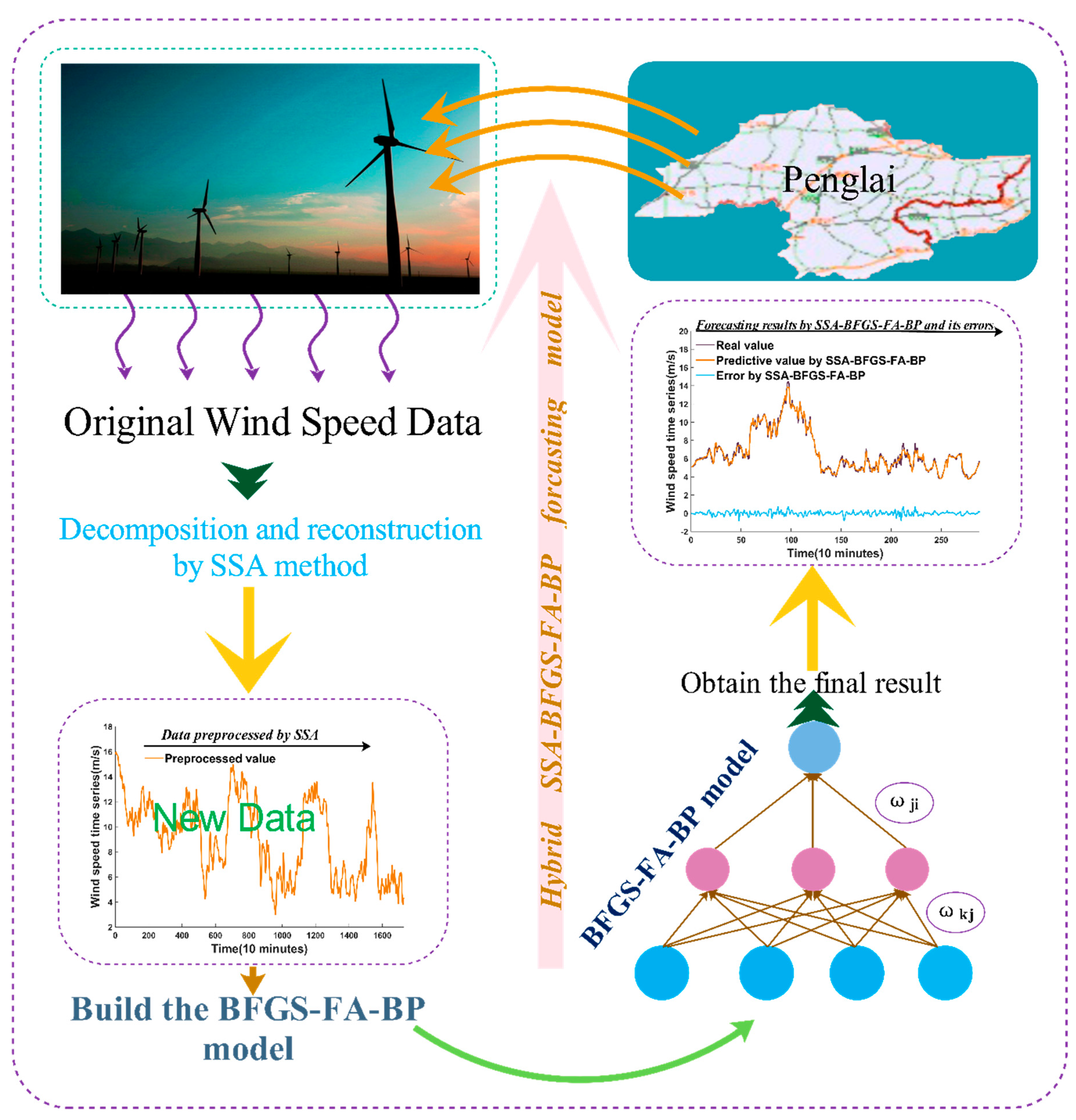
The BP algorithm is selected as the forecasting method to forecast the wind speed time series in this paper. However, because of its unstable structure, we could not obtain more accurate forecasting results with minor error; therefore, it is important to determine the optimal parameters and threshold values of the BP network to promote the predictive effectiveness. BFGF-FA is proposed to determine the weight and threshold. In addition, large amounts of noise present in the original wind sequence will lead to a poor forecasting performance. Therefore, we choose the SSA to remove the noise from the raw time sequence. The corresponding basic procedures are presented as follows, and are depicted in Figure 2.
Step 1. SSA is used to remove the noise from the raw data. It also aims to remove the high frequency of the original sequence after decomposing, and then reconstructs them into new experimental data.
Step 2. BFGS-FA is used to determine the weight and threshold of the BP neural network. Thus, the ability of the global optimization of the BP algorithm is greatly promoted.
Step 3. The optimized BP neural network is applied to predict the wind speed time sequence.
Step 4. The proposed hybrid model indeed outperforms the single models in forecasting time sequences based on historical values. Multi-step forecasting also proves that the proposed hybrid method has a higher effectiveness, and their forms can be described as follows:
- (1).
- One-step prediction: The predictive value is calculated on the basis of the past time sequence , where t is the sample size of the wind speed time sequence.
- (2).
- Two-step prediction: The predictive value is calculated on the basis of the past time sequence and the former predictive value .
- (3).
- Three-step prediction: The predictive value is calculated on the basis of the past time sequence and the former predictive value and .
- (4).
- Higher-step forecasting value will be obtained on the basis of the above form.
2.7. Testing Method
In this paper, we also employed a testing method called the Diebold-Mariano (DM) test to estimate the proposed model.
The Diebold-Mariano (DM) test [56], which is focused on predictive accuracy, compares and evaluates the predictive effectiveness of the proposed hybrid method with other simple models. In practical applications, there will be two or more time sequence models available for predicting a specific variable of interest.
Real values:
Two predictions:
The prediction errors according to the two models can be described as follows:
and:
The precision of each forecasting model is evaluated by an appropriate loss function, .
The most widespread and available loss function is square error loss, and its formulation is as follows:
Square error loss:
The DM test statistic assesses the prediction according to the random loss function L(p):
where S2 is the estimated value of the variance of , and the null hypothesis is:
in contrast, the alternative hypothesis is:
Under the null hypothesis, the two predictions possess uniform precision. In contrast, the alternative hypothesis has different standards, namely, the two predictions differ in accuracy. If the null hypothesis is right, the Diebold-Mariano statistic will be an asymptotically standard normal distribution N(0,1). The null hypothesis should not be refused if the calculation of DM statistic falls inside the interval [−Zα/2, Zα/2], otherwise we must reject it; that is, the reject region is (−∞,−Zα/2)&(Zα/2,+∞), which is defined as follows:
where Zα/2 is the positive Z-value from the standard normal table according to half of the confidence level of the experiment.
3. Experimental Design and Results
In this section, the wind speed data gathered from three sites are forecast by the developed hybrid method. The data location and effectiveness of the prediction estimation standard are also presented. All the experiments in this paper were conducted in MATLAB R2014b on Windows 7 with 3.30 GHz Intel (R) Core (TM) i5 4590 CPU, 64 bit and 8 GB RAM.
3.1. Data Sets
The hybrid SSA-BFGS-FA-BP method was tested using data from experiments of wind speed prediction time sequences at three sites. A data set gathered at 10-min intervals from Penglai city, Shandong province, China, was used. Figure 3a displays the geographical position of Penglai city in China.
In this study, wind speeds are taken from three different sites, and we chose 1728 of them as observation values. Of these, 1440 values were used to train the network, and the remaining 288 values were selected as the testing set for each station.
The original data from the three sites are shown in Figure 3b, which illustrates the inordinance, wave, and mutability of the original time series.
3.2. Forecast Error Metrics
Forecasting errors are applied to assess the ability of the applied forecasting approaches and to evaluate the effectiveness of the proposed method on account of on-site/true measures.
The metric equations in Table 4 show us the universal error index applied to most forecasting models for renewables. The mean absolute error (MAE), the root mean square error (RMSE) [57], and the mean absolute percentage error (MAPE) are used to estimate the forecasting effectiveness of the proposed method. They are denoted as follows:
and are the true value and the predicted value, respectively. T is the total number of elements in this data array. The MAE depends on and , the RMSE depends on and , and furthermore, the MAPE gives the relative error between and . Quantified by these three frequently used indices, we can clearly and concisely perceive the difference between the predicted and exact wind speed values. A smaller difference value indicates that the forecasting method has a better performance. Nevertheless, MAPE, a unit-free estimator, has better sensitivity for small-scale variation, does not reveal some weak characteristics of data, such as asymmetry, and has lower abnormal value protection. Therefore, a better MAPE will be chosen as the standard in this paper.
3.3. Comparison Method and Its Corresponding Results
Our main contribution is not only to provide an optimization algorithm, but also to propose a novel hybrid wind speed forecasting model. Experimental results prove that the proposed method can be perfectly used for short-term wind speed forecasting, and that it has considerable practical value and strong operability in wind farms and grid management. In addition, we performed a comparative experiment to compare the proposed model with other forecasting approaches, and the corresponding results are presented in Table 5, revealing that the proposed hybrid method achieves higher forecasting accuracy than the other methods.
3.4. Case Studies
This study consists of three classic experiments. Each of them is grouped into two sections, one of which uses the primary wind speed data and the other applies data preprocessed by the SSA approach. Original data are forecast by the single BP algorithm, and the BP algorithm is optimized using combined BFGS-FA (BFGS-FA-BP); decomposed data are also predicted by the single BP and BFGS-FA (BFGS-FA-BP).
The two model aim to compare the single BP with the optimized BFGS-FA-BP to determine the performance of the hybrid method. The parameters of SSA are presented in Table 6.
3.4.1. Case Study 1
In this section, all results will be clearly demonstrated in the figures and tables to reveal the effectiveness of each model. First, the predicted values of wind speed in the three locations are presented in Table 7, Table 8 and Table 9. Considering the random disturbances of the forecasts, it is necessary to repeat each experiment many times to ensure the reliability of results. Therefore, in our study, we performed each experiment 20 times and then used the average values as the final results, to make sure that the results are dependable.
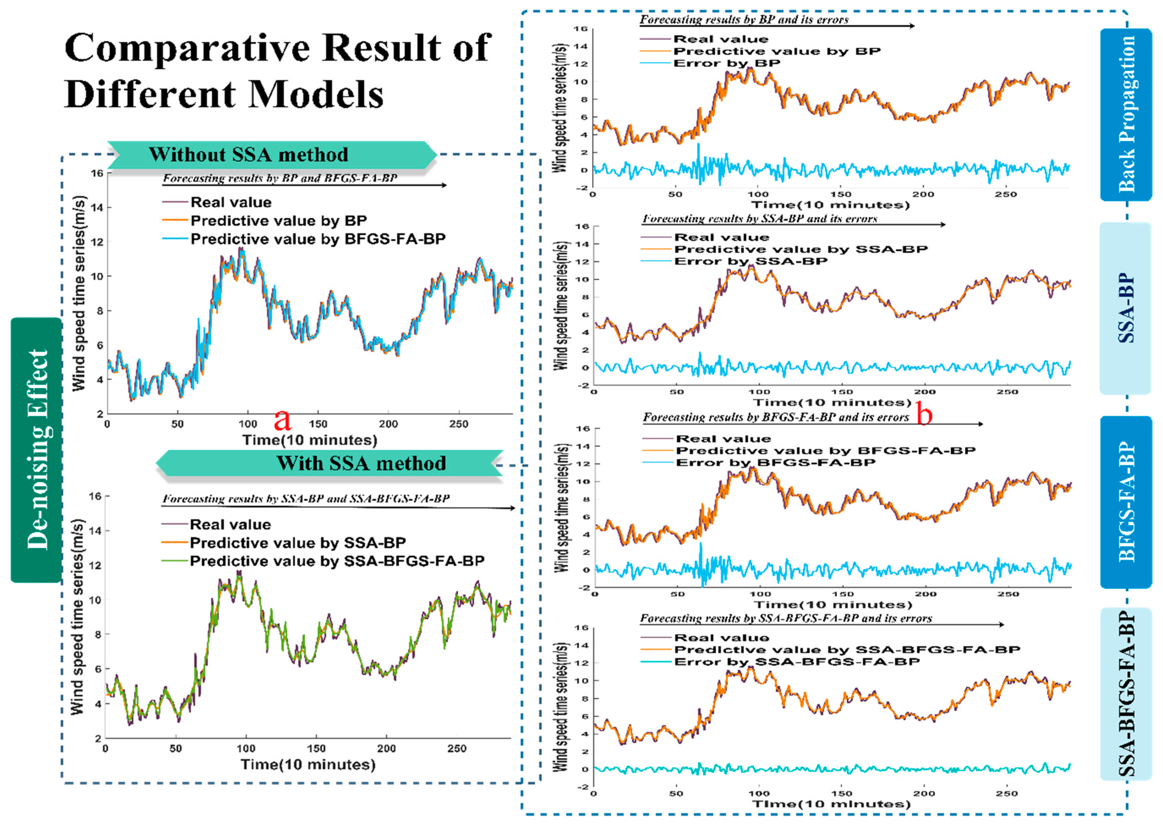
Figure 4a shows the data of the estimated performance with and without using the SSA approach at site 1. The effectiveness of the experiment that used real values is displayed at the top left side of the chart, and was forecast by models without using the SSA approach. The effectiveness of the experiment that used processed data is described at the bottom left side of the Figure, and was forecast by models using the SSA approach. We can conclude from the Figure that the SSA-BP model predicts values close to the true values, especially SSA-BFGS-FA-BP. In other words, the experiment that used processed data showed better performance than the other.
Figure 4b shows the difference between the forecast values and the exact values collected from site 1, and their corresponding errors. We can clearly see that the error of the SSA-BFGS-FA-BP model is much lower than that of the BP, BFGS-FA-BP, and SSA-BP models, which implies that the SSA-BFGS-FA-BP method performs much better than other models.
3.4.2. Results of Analysis
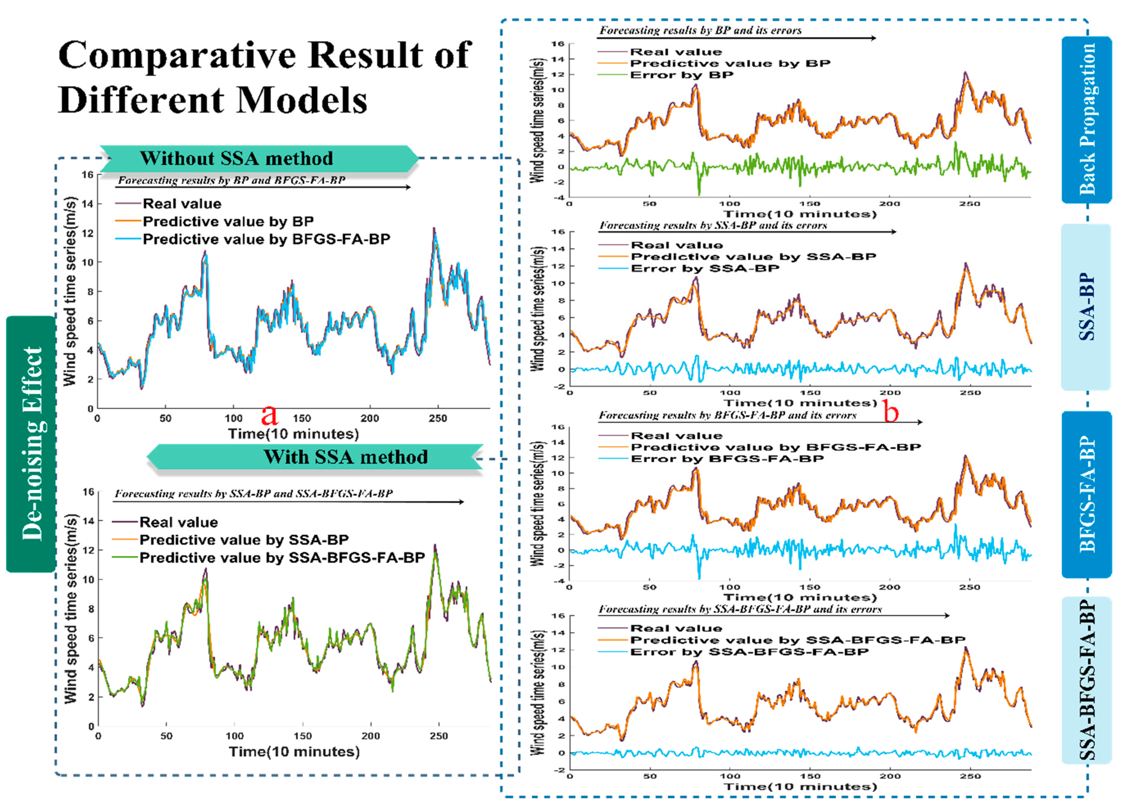
In this section, another two samples are described in Figure 5a and Figure 6a, whose predictive performance with and without using the SSA method are compared. Furthermore, Figure 5b and Figure 6b illustrate the difference between the forecast values and the real values collected from the other two sites and their corresponding errors.
Similar to what was described above, and as shown in Figure 5a and Figure 6a, the BP and BFGS-FA-BP models closely approached the actual values, but the SSA-BP model and especially the SSA-BFGS-FA-BP model performed much better in forecasting. Therefore, we can conclude that the experiment using the SSA approach outperforms the other. As revealed in Figure 5b and Figure 6b, the deviations of the SSA-BFGS-FA-BP model are much smaller than those of the BP, BFGS-FA-BP, and SSA-BP models. In particular, it is very clear that the SSA-BFGS-FA-BP model gets extremely close to the exact wind speed, and has higher performance than the other three models.
To test the accuracy of the experiment and guarantee the practicability and feasibility of the developed method, we performed another three experiments. As shown in Table 10, data were taken during four seasons (spring, summer, autumn, and winter) from a fixed location to verify the stability of the model. The results presented in this indicate that (1) the variance of the proposed hybrid SSA-BFGS-FA-BP method is minimal; and (2) the predicted value of the hybrid SSA-BFGS-FA-BP model is closer to the true value, having higher stability than the other three models.
In another experiment, the new predicted value based on historical data was used as the new real value to test. Using this, we performed three-step iterative, six-step iterative, and twelve-step iterative experiments. The final experimental results are shown in Table 10. The results indicate that the variance of the hybrid SSA-BFGS-FA-BP model is smaller, and that the predicted value within six steps of hybrid SSA-BFGS-FA-BP model is closer to the true value, having higher stability than the other three models. However, in the 12-step iterative experiment, the proposed SSA-BFGS-FA-BP model did not show better accuracy than the other three models. This indicates that the optimal results will be worse with an increase in the number of iterations beyond a certain extent, because of the increase in randomness. This also verifies that, with an increase in the number of iterations, the accuracy of prediction is low and the deviation is high.
Finally, we collected data at different time intervals (10, 30 and 60-min intervals) from a fixed location to conduct an experiment, and the results of the experiment are shown in Table 11. We can conclude from the table that the effects of the optimization method will run into a bottleneck when the time interval of the data becomes too great. The hybrid SSA-BFGS-FA-BP model did not show a better performance. The error of forecasting reached a high value when the time interval was so long.
In conclusion, the SSA-BFGS-FA-BP has much higher effectiveness than the single BP, BFGS-FA-BP, and SSA-BP models. We can confirm that the hybrid SSA-BFGS-FA-BP model can make a more accurate prediction on account of the original time sequence.
3.5. The Results of the DM Test
The DM test was employed to verify the levels of accuracy forecasted by the proposed hybrid method and the other three single models. Table 12 shows that the values of the DM statistics between the proposed hybrid model and the BP, SSA-BP and BFGS-FA-BP models are 8.1064, 8.0468 and 8.1696, respectively. Under a 1% confidence level, the upper limit value is much smaller than these DM statistics; therefore, we cannot accept the null hypothesis and we have to admit the alternative hypothesis. Thus, we can conclude that the hybrid method outperforms the other single methods.
Remark.
We could learn from the results in terms of estimations on the basis of the DM test that the novel hybrid method achieves a more precise and stable prediction capacity than the other three models, and that the forecasting effectiveness of the hybrid method differs from that of the BP, SSA-BP, and BFGS-FA-BP models.
4. Discussion
In this section, we initially discuss the application of SSA in preprocessing the original data, which influences the forecasting performance. We also examine the MAPEs of decreased relative percentage (DRP) between the proposed model and other forecasting approaches. Furthermore, we present and discuss variations of the data selection.
4.1. Data Pre-Processing
In general, plenty of noise and high-frequency time series lie in the raw wind speed time sequence. Therefore, the decomposition of the original data sequence is a significant process in data filtering. This can always effectively enhance the prediction accuracy of the model to obtain better forecast results. Through the comparison between BP and SSA-BP, we can assess the effectiveness of the data pre-processing using a new metric called DRP (%), and its corresponding defining equation is summarized as follows:
The experimental results show that the method significantly enhances the forecasting effectiveness: it decreases the MAPE by 32.8%, 29.3% and 30.7% for site 1, site 2 and site 3, respectively.
4.2. Neural Networks
In the field of practical engineering, the quality of a model depends on its effectiveness, rather than its complexity. However, the question of how to seek an effective forecasting method to enhance performance is not only a problem that is in urgent need of a solution, but also a critical problem in the field of forecasting. The relevant study [58] showed that there was no one unified model for forecasting time series, and model effectiveness under different circumstances should be analyzed and understood, with incremental improvements being made on the basis of the knowledge gained; therefore, it is impossible to find one model to solve all forecasting problems.
Thus, our attention should be more focused on the DRP of the error forecast by different approaches using different data sets, in order to find a relatively good model for forecasting wind speed time series. Through analyzing the difference between the proposed model and the other comparative models, we can find that the proposed model improves effectiveness by 38.4654%, 35.5391 and 37.9645% for site 1, site 2 and site 3, respectively. The detailed results are presented in Table 13. From the Table, we can see that the developed method has a very good performance in decreasing wind speed forecasting error.
4.3. Data Selection
According to the forecast results, the 10-min interval data sequence achieves the best forecasting effectiveness for all three observation sites, with an MAPE of approximately 6%; therefore, the proposed hybrid model shows excellent performance in forecasting the wind speed time sequence at 10-min intervals. The 10-min interval time series at each observation site decreases the forecasting error by 12.59%, 10.14% and 11.41%, respectively.
For the time series data with a 60-min interval, the forecast results are good for all three observation sites, while the forecasting performance is worse than for the data with a 10-min interval. Therefore, the SSA-BFGS-FA-BP is more applicable to forecasting the wind speed time sequence with a 10-min interval, and the data selection will have a serious effect on forecasting effectiveness. However, regardless of the time interval, the forecasting effectiveness is in an acceptable range. Many works apply the wind speed series with time resolutions including 10, 30 and 60 min for the purpose of the forecast, which is representative for studying wind speed forecasting. The detailed comparison results are presented in Table 14.
5. Conclusions and Future Work
As a kind of non-polluting and renewable energy source, wind energy has been increasingly applied in the development of industry and agriculture, and its forecasting is becoming increasingly important for wind farms. Recently, academia and wind farm projects have been gradually paying more attention to wind speed forecasting. Perfect prediction can not only reduce costs and enhance personal safety, but also help wind farm management develop more effective programs. The accuracy of a model is as important as its stability in forecasting. It is of great interest to propose an outstanding method for wind speed prediction with high accuracy and long-term stability. Nevertheless, wind speed prediction has been generally considered a challenging task in terms of the effects of various intangible factors, such as temperature, location, tides, atmospheric pressure, and other factors. In this paper, to overcome these difficulties, a hybrid model that combines the SSA approach, BFGS-FA algorithm, and BP method is presented.
The results based on evaluation criteria such as the MAE, RMSE, MAPE and a statistical test are shown in a sequence of charts, in which the superior qualities of the developed hybrid method are revealed most vividly. From the data in the tables and figures, we can draw the conclusion that the proposed hybrid method achieves the best forecasting effectiveness and a higher stability and reliability.
SSA is a practical decomposition approach, which can remove the noise from the raw data, leaving the principal component for forecasting. The BP model, based on feed forward neural networks, has increasingly turned into a fairly distinguished tool. It is shown that the BP model can get its final predictive results in a remarkably short time.
In brief, the hybrid model always has the lowest MAPE value compared with other single forecasting methods, which implies that the hybrid method has the best performance and higher reliability. Improvements in forecasting accuracy and stability can not only help to save large amounts of energy and money, but also help to reduce the time the system requires. The experiments performed in the present study show that the developed hybrid method is a potential algorithm with high accuracy. In addition, the hybrid method could be applied to other fields of practical engineering, such as electric load forecasting, stock price prediction, and solar resource forecasting.
Acknowledgments
This work was funded by the National Natural Science Foundation of China (Grant No. 71573034).
Author Contributions
Zeng Wang wrote the whole manuscript, and carried out the data analysis; Ping Jiang gave overall guidance; Kequan Zhang and Wendong Yang conducted the programming and part of the data processing.
Conflicts of Interest
The authors declare no conflict of interest.
Abbreviations
| ARIMA | auto-regressive integrated moving average | Genmax | the maximum number of iterations |
| BFGS | Broyden-Fletcher-Goldfarb-Shanno | MAPE | mean absolute percentage error |
| MLP | multi-layer perceptron | MAE | mean absolute error |
| BP | back propagation | RMSE | root mean square error |
| RBF | radial basis function | betamin | minimum value of beta |
| RNN | Recurrent Neural Networks | gamma | absorption coefficient |
| BPA | back propagation algorithm | DM | Diebold-Mariano |
| PSO | particle swarm optimization | SVM | Support Vector Machine |
| ANN | artificial neural network | T | the length of time series |
| FA | firefly algorithm | Valuemin | the minimum real value |
| BPNN | back propagation neural network | K | the length of the trajectory matrix |
| CS | cuckoo search | SVD | singular value decomposition |
| MCS | modified cuckoo search | GA | genetic algorithm |
| Valueactual | real value | H0 | the null hypothesis |
| SSA | singular spectrum analysis | H | continuous function |
| EMD | empirical mode decomposition | WD | wavelet decomposition |
| Valuenormalized | data after linear transformation | H1 | the alternative hypothesis |
| Valuemax | the maximum real value | Zα/2 | upper (or positive) Z-value |
| Zij | an element of a generic matrix Z | DRP | decreased relative percentage |
| ENN | Elman neural network | WNN | Wavelet neural network |
Appendix A
| Algorithm A1. BFGS. | |||
| Parameters: | |||
| δ–the tolerance of convergence. t –present iterative times. | |||
| Genmax–the max iterative times. | |||
| 1: | /*Initialize the convergence tolerance δ and present iterative times.*/ | ||
| 2: | Set the convergence tolerance δ > 0, t ← 0 | ||
| 3: | Assess the inverse matrix of Hessian matrix at an initial value x° | ||
| 4: | WHILE (t < Genmax) RUN | ||
| 5: | /* Compute search path.*/ | ||
| 6: | |||
| 7: | /* Compute step size.*/ | ||
| 8: | |||
| 9: | /*Obtain the new iteration.*/ | ||
| 10: | |||
| 11: | IF(xPt+1 > xPup) WELL | ||
| 12: | Xpt+1 = xpup | ||
| 13: | ELSE IF(xpt+1 < xpl°) WELL | ||
| 14: | Xpt+1 = xpl° | ||
| 15: | END | ||
| 16: | Compute Dt+1 | ||
| 17: | Set t←t+1 | ||
| 18: | END | ||
Appendix B
| Algorithm A2. FA. | |||||
| Input: | |||||
| –a series of data for training. | |||||
| –a series of data for verifying. | |||||
| Output: | |||||
| xbthe corresponding value of x when it acquires the optimal fitness among all fireflies. | |||||
| Parameters: | |||||
| Genmax–the max iterative times. n–the total number of fireflies. | |||||
| Fp–the fitness function according to firefly p. xp–nest p. g–the present number of iterations. | |||||
| Lp–the brightness of firefly p. d–the dimension of the parameter. | |||||
| 1:: | /* Define all the parameters related to FA.*/ | ||||
| 2: | /* Initialize the species of fireflies at random.*/ | ||||
| 3: | FOR p = 1:n RUN | ||||
| 4: | Assess the relevant fitness function Fp | ||||
| 5: | END | ||||
| 6: | /* Confirm light intensity. */ | ||||
| 7: | FOR p = 1:n RUN | ||||
| 8: | Confirm the brightness Lp through F(xp) | ||||
| 9: | END | ||||
| 10: | WHILE (g < Genmax) RUN | ||||
| 11: | FOR p = 1:n RUN | ||||
| 12: | FOR q = 1:n RUN | ||||
| 13: | /* Adjust the firefly from p to q in any direction.*/ | ||||
| 14: | IF (Lq > Lp) WELL | ||||
| 15: | |||||
| 16: | |||||
| 17: | END | ||||
| 18: | Attraction changes with the distance r via | ||||
| 19: | END | ||||
| 20: | END | ||||
| 21: | /*Renew the best nest xm of the d generation*/ | ||||
| 22: | FOR p = 1:n RUN | ||||
| 23: | IF (Fm < Fb) WELL | ||||
| 24: | xb ← xm; | ||||
| 25: | END | ||||
| 26: | END | ||||
| 27: | END | ||||
| 28: | RETURN xb | ||||
Appendix C
| Algorithm A3. BFGS-FA. | |||||
| Input: | |||||
| –a series of data for training. | |||||
| –a series of data for verifying | |||||
| Output: | |||||
| xb–the corresponding value of x when it acquires the optimal fitness among all fireflies. | |||||
| Parameters: | |||||
| Genmax–the max iterative times. n–the total number of fireflies. | |||||
| Fp–the fitness function according to firefly p. xp–nest p. g–the present number of iterations. | |||||
| Lp–the brightness of firefly p. d–the dimension of the parameter. | |||||
| 1: | /*Define all the parameters related to FA and BFGS.*/ | ||||
| 2: | /* Initialize population of n fireflies at random.*/ | ||||
| 3: | FORp = 1:nRUN | ||||
| 4: | Assess the relevant fitness function Fp | ||||
| 5: | END | ||||
| 6: | /* Confirm light intensity*/ | ||||
| 7: | FOR p = 1:n RUN | ||||
| 8: | Confirm brightness Lp through F(xp) | ||||
| 9: | END | ||||
| 10: | WHILE (g < Genmax ) RUN | ||||
| 11: | FOR p = 1:n RUN | ||||
| 12: | FOR q = 1:n RUN | ||||
| 13: | /* Adjust the firefly from p to q in any direction */ | ||||
| 14: | IF(Lq > Lp) WELL | ||||
| 15: | |||||
| 16: | |||||
| 17: | END | ||||
| 18: | Attraction changes with the distance r via | ||||
| 19: | Apply BFGS to help to renew the new site of fireflies quickly. | ||||
| 20: | /*Assess the new position and renew the new light intensity Lp.*/ | ||||
| 21: | FOR p = 1:n RUN | ||||
| 22: | Assess the relevant fitness function Fp | ||||
| 23: | END | ||||
| 24: | /* Update the brightness*/ | ||||
| 25: | FOR p = 1:n RUN | ||||
| 26: | Confirm the brightness Lp through F(xp) | ||||
| 27: | END | ||||
| 28: | END | ||||
| 29: | END | ||||
| 30: | /*Update best nest xm of the d generation.*/ | ||||
| 31: | FOR p = 1:nRUN | ||||
| 32: | IF(Fm < Fb)WELL | ||||
| 33: | xb ← xm | ||||
| 34: | END | ||||
| 35: | END | ||||
| 36: | END | ||||
| 37: | RETURN xb | ||||
References
- Manzano-Agugliaro, F.; Zapata-Sierra, A.; Herna, Q. The wind power of Mexico. Renew. Sustain. Energy Rev. 2010, 14, 2830–2840. [Google Scholar]
- Manzano-Agugliaro, F.; Sanchez-Muros, M.J.; Barroso, F.G.; Martínez-Sánchez, A.; Rojo, S. Insects for biodiesel production. Renew. Sustain. Energy Rev. 2012, 16, 3744–3753. [Google Scholar] [CrossRef]
- Hernández-Escobedo, Q.; Saldaña-Flores, R.; Rodríguez-García, E.R. Wind energy resource in Northern Mexico. Renew. Sustain. Energy Rev. 2014, 32, 890–914. [Google Scholar] [CrossRef]
- World Wind Energy Association (2009). World Wind Energy Report. Available online: http://www.wwindea.org/home/images/stories/worldwindenergyreport2009_s.pdf (accessed in 10 March 2017).
- Hernandez-Escobedo, Q.; Manzano-Agugliaro, F.; Gazquez-Parra, J.A.; Zapata-Sierra, A. Is the wind a periodical phenomenon? The case of Mexico. Renew. Sustain. Energy Rev. 2011, 15, 721–728. [Google Scholar] [CrossRef]
- Montoya, F.G.; Manzano-Agugliaro, F.; López-Márquez, S.; Hernández-Escobedo, Q.; Gil, C. Wind turbine selection for wind farm layout using multi-objective evolutionary algorithms. Expert Syst. Appl. 2014, 41, 6585–6595. [Google Scholar] [CrossRef]
- Ernst, B.; Oakleaf, B.; Ahlstrom, M.L.; Lange, M.; Moehrlen, C.; Lange, B.; Focken, U.; Rohrig, K. Predicting the wind. IEEE Power Energy Mag. 2007, 5, 78–89. [Google Scholar] [CrossRef]
- Liu, H.; Tian, H.Q.; Liang, X.F.; Li, Y.F. Wind speed forecasting approach using secondary decomposition algorithm and Elman neural networks. Appl. Energy 2015, 157, 183–194. [Google Scholar] [CrossRef]
- Al-Yahyai, S.; Charabi, Y.; Gastli, A. Review of the use of numerical weather prediction (NWP) models for wind energy assessment. Renew. Sustain. Energy Rev. 2010, 14, 3192–3198. [Google Scholar] [CrossRef]
- Amral, N.; Ozveren, C.S.; King, D. Short term load forecasting using Multiple Linear Regression. In Proceedings of the 42th International Universities Power Engineering Conference, Brighton, UK, 4–6 September 2007; pp. 1192–1198. [Google Scholar]
- Li, W.; Zhang, Z.G. Based on time sequence of ARIMA model in the application of short-term electricity load forecasting. In Proceedings of the International Conference on Research Challenges in Computer Science, Shanghai, China, 28–29 December 2009; pp. 11–14. [Google Scholar]
- Christiaanse, W.R. Short-Term Load Forecasting Using General Exponential Smoothing. IEEE Trans. Power Appar. Syst. 1971, PAS-90, 900–911. [Google Scholar] [CrossRef]
- Irisarri, G.D.; Widergren, S.E.; Yehsakul, P.D. On-line load forecasting for energy control center application. IEEE Trans. Power Appar. Syst. 1982, PAS-101, 71–78. [Google Scholar] [CrossRef]
- Du, P.; Jin, Y.; Zhang, K. A Hybrid Multi-Step Rolling Forecasting Model Based on SSA and Simulated Annealing—Adaptive Particle Swarm Optimization for Wind Speed. Sustainability 2016, 8, 754. [Google Scholar] [CrossRef]
- Hu, Y.C. Pattern classification by multi-layer perceptron using fuzzy integral-based activation function. Appl. Soft Comput. 2010, 10, 813–819. [Google Scholar] [CrossRef]
- Peeling, S.M.; Moore, R.K. Isolated digit recognition experiments using the multi-layer perceptron. Speech Commun. 1988, 7, 403–409. [Google Scholar] [CrossRef]
- Fan, X.; Wang, L.; Li, S. Predicting chaotic coal prices using a multi-layer perceptron network model. Resour. Policy 2016, 50, 86–92. [Google Scholar] [CrossRef]
- Ganotra, D.; Joseph, J.; Singh, K. Profilometry for the measurement of three-dimensional object shape using radial basis function, and multi-layer perceptron neural networks. Opt. Commun. 2002, 209, 291–301. [Google Scholar] [CrossRef]
- Beigy, H.; Meybodi, M.R. Backpropagation algorithm adaptation parameters using learning automata. Int. J. Neural Syst. 2001, 11, 219–228. [Google Scholar] [CrossRef] [PubMed]
- Jain, A.; Srinivas, E.; Rauta, R. Short Term Load Forecasting using Fuzzy Adaptive Inference and Similarity. In Proceedings of the World Congress on Nature & Biologically Inspired Computing, Coimbatore, India, 9–11 December 2009. [Google Scholar]
- Kumar, R.; Aggarwal, R.K.; Sharma, J.D. Comparison of regression and artificial neural network models for estimation of global solar radiations. Renew. Sustain. Energy Rev. 2015, 52, 1294–1299. [Google Scholar] [CrossRef]
- Rather, A.M.; Agarwal, A.; Sastry, V.N. Recurrent neural network and a hybrid model for prediction of stock returns. Expert Syst. Appl. 2015, 42, 3234–3241. [Google Scholar] [CrossRef]
- Cardoso, M.C.; Silva, M.; Vellasco, M.M.B.R.; Cataldo, E. Quantum-inspired features and parameter optimization of Spiking Neural Networks for a case study from atmospheric. Procedia Comput. Sci. 2015, 53, 74–81. [Google Scholar] [CrossRef]
- Sheela, K.G.; Deepa, S.N. An Intelligent Computing Model for Wind Speed Prediction in Renewable Energy Systems. Procedia Eng. 2012, 30, 380–385. [Google Scholar]
- Liu, N.; Tang, Q.; Zhang, J.; Fan, W.; Liu, J. A hybrid forecasting model with parameter optimization for short-term load forecasting of micro-grids. Appl. Energy 2014, 129, 336–345. [Google Scholar] [CrossRef]
- Wang, J.; Zhu, S.; Zhang, W.; Lu, H. Combined modeling for electric load forecasting with adaptive particle swarm optimization. Energy 2010, 35, 1671–1678. [Google Scholar] [CrossRef]
- Xiao, L.; Wang, J.; Hou, R.; Wu, J. A combined model based on data pre-analysis and weight coefficients optimization for electrical load forecasting. Energy 2015, 82, 524–549. [Google Scholar] [CrossRef]
- Zhao, J.; Guo, Z.H.; Su, Z.Y.; Zhao, Z.Y.; Xiao, X.; Liu, F. An improved multi-step forecasting model based on WRF ensembles and creative fuzzy systems for wind speed. Appl. Energy 2016, 162, 808–826. [Google Scholar] [CrossRef]
- Qin, S.; Liu, F.; Wang, J.; Song, Y. Interval forecasts of a novelty hybrid model for wind speeds. Energy Reports 2015, 1, 8–16. [Google Scholar] [CrossRef]
- Wang, J.; Song, Y.; Liu, F.; Hou, R. Analysis and application of forecasting models in wind power integration: A review of multi-step-ahead wind speed forecasting models. Renew. Sustain. Energy Rev. 2016, 60, 960–981. [Google Scholar] [CrossRef]
- Xiao, L.; Wang, J.; Yang, X.; Xiao, L. A hybrid model based on data preprocessing for electrical power forecasting. Int. J. Electr. Power Energy Syst. 2015, 64, 311–327. [Google Scholar] [CrossRef]
- Xu, Y.; Yang, W.; Wang, J. Air quality early-warning system for cities in China. Atmos. Environ. 2017, 148, 239–257. [Google Scholar] [CrossRef]
- Xiao, L.; Shao, W.; Liang, T.; Wang, C. A combined model based on multiple seasonal patterns and modified firefly algorithm for electrical load forecasting. Appl. Energy 2016, 167, 135–153. [Google Scholar] [CrossRef]
- Fister, I.; Yang, X.S.; Brest, J. A comprehensive review of firefly algorithms. Swarm Evolut. Comput. 2013, 13, 34–46. [Google Scholar] [CrossRef]
- Azad, S.K. Optimum Design of Structures Using an Improved Firefly Algorithm. Iran Univ. Sci.Technol. 2011, 1, 327–340. [Google Scholar]
- Wang, J.; Qin, S.; Zhou, Q.; Jiang, H. Medium-term wind speeds forecasting utilizing hybrid models for three different sites in Xinjiang, China. Renew. Energy 2015, 76, 91–101. [Google Scholar] [CrossRef]
- Guo, Z.; Zhao, W.; Lu, H.; Wang, J. Multi-step forecasting for wind speed using a modified EMD-based artificial neural network model. Renew. Energy 2012, 37, 241–249. [Google Scholar] [CrossRef]
- Chau, K.W.; Wu, C.L. A hybrid model coupled with singular spectrum analysis for daily rainfall prediction. J. Hydroinform. 2010, 12, 458–473. [Google Scholar] [CrossRef]
- Hu, J.; Wang, J.; Zeng, G. A hybrid forecasting approach applied to wind speed time series. Renew. Energy 2013, 60, 185–194. [Google Scholar] [CrossRef]
- Zhang, C.; Wei, H.; Xie, L.; Shen, Y.; Zhang, K. Direct interval forecasting of wind speed using radial basis function neural networks in a multi-objective optimization framework. Neurocomputing 2016, 205, 53–63. [Google Scholar] [CrossRef]
- Wang, J.; Zhang, W.; Li, Y.; Wang, J.; Dang, Z. Forecasting wind speed using empirical mode decomposition and Elman neural network. Appl. Soft Comput. 2014, 23, 452–459. [Google Scholar] [CrossRef]
- Yao, C.; Gao, X.; Yu, Y. Wind speed forecasting by wavelet neural networks: A comparative study. Math. Probl. Eng. 2013, 9, 681–703. [Google Scholar] [CrossRef]
- Wang, S.; Zhang, N.; Wu, L.; Wang, Y. Wind speed forecasting based on the hybrid ensemble empirical mode decomposition and GA-BP neural network method. Renew. Energy 2016, 94, 629–636. [Google Scholar] [CrossRef]
- Yang, Z.; Wang, J. Multi-step wind speed forecasting using a novel model hybridizing singular spectrum analysis, modified intelligent optimization and rolling Elman neural network. Math. Probl. Eng. 2016, 2016, 1–30. [Google Scholar]
- McCulloch, W. S.; Pitts, W.H. A logical calculus of ideas imminent in nervous activity. BullMath. Biophy. 1943, 5, 115–133. [Google Scholar]
- Yan, P.; Zhang, C. Artificial Neural Network and Simulating-Evolution Computation; Tsinghua University Press: Beijing, China, 2000. [Google Scholar]
- Bazaraa, M.S.; Sherali, H.D.; Shetty, C.M. Nonlinear Programming: Theory and Algorithms; Wiley: Hoboken, NJ, USA, 1993; Volume 3. [Google Scholar]
- Yang, X.S. Firefly algorithms for multimodal optimization. In Lecture Notes in Computer Science (including subseries Lecture Notes in Artificial Intelligence and Lecture Notes in Bioinformatics); Springer: Berlin/Heidelberg, Germany, 2009; Volume 5792, pp. 169–178. [Google Scholar]
- Bendjeghaba, O.; Boushaki, S.I.; Zemmour, N. Firefly algorithm for optimal tuning of PID controller parameters. In Proceedings of the 2013 fourth International Conference on Power Engineering, Energy and Electrical Drives (POWERENG), Istanbul, Turkey, 13–17 May 2013; pp. 1293–1296. [Google Scholar]
- Lohrer, M. A Comparison between the Firefly Algorithm and Particle Swarm Optimization. Ph.D. Thesis, University of Oakland, Rochester, MI, USA, 2013. [Google Scholar]
- Beneki, C.; Eeckels, B.; Leon, C. Signal extraction and forecasting of the UK tourism income time series: A singular spectrum analysis approach. J. Forecast. 2012, 31, 391–400. [Google Scholar] [CrossRef]
- Elsner, J.B.; Tsonis, A.A. Singular Spectrum Analysis: A New Tool in Time Series Analysis; Springer: Berlin, Germany, 1996; Volume 1283, pp. 932–942. [Google Scholar]
- Golyandina, N.; Nekrutkin, V.; Zhigljavsky, A. Analysis of Time Series Structure: SSA and Related Techniques; Chapman Hall/CRC: Boca Raton, FL, USA, 2001. [Google Scholar]
- Hassani, H. Singular Spectrum Analysis: Methodology and Comparison. J. Data Sci. 2007, 5, 239–257. [Google Scholar]
- Hassani, H.; Heravi, S.; Zhigljavsky, A. Forecasting European industrial production with singular spectrum analysis. Int. J. Forecast. 2009, 25, 103–118. [Google Scholar] [CrossRef]
- Diebold, F.X.; Mariano, R.S. Comparing Predictive Accuracy. J. Bus. Econ. Stat. 1995, 13, 253–265. [Google Scholar] [CrossRef]
- Inman, R.H.; Pedro, H.T.C.; Coimbra, C.F.M. Solar Forecasting Methods for Renewable Energy Integration. Prog. Energy Combust. Sci. 2013, 39, 535–576. [Google Scholar] [CrossRef]
- Moghram, I.; Rahman, S. Analysis and evaluation of five short-term load forecasting techniques. IEEE Trans. Power Syst. 1989, 4, 1484–1491. [Google Scholar]
Figure 1.
Topology structure and flow chart of BP neural network and the flow chart and structure of the combined BFGS-FA Algorithm.
Figure 1.
Topology structure and flow chart of BP neural network and the flow chart and structure of the combined BFGS-FA Algorithm.

Figure 2.
The flow chart of the hybrid SSA-BFGS-FA-BP model.

Figure 3.
Geographical position of the survey regions and actual values of three stations.
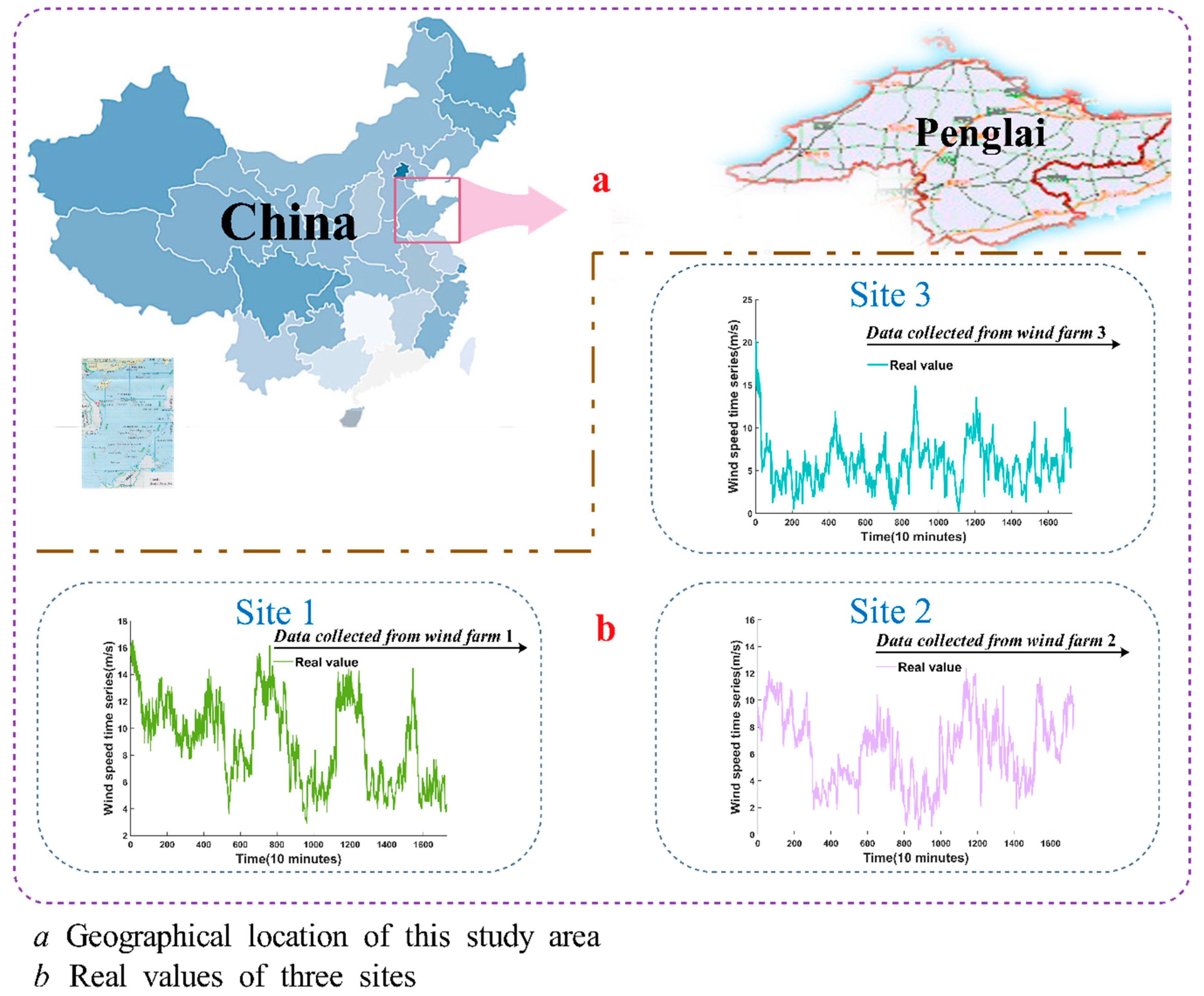
Figure 4.
The forecast results for wind speed collected from site 1 at 10-min intervals. (a) The forecast effect without SSA algorithm and with SSA algorithm; (b) The comparison between the forecast values and raw data and their corresponding errors.
Figure 4.
The forecast results for wind speed collected from site 1 at 10-min intervals. (a) The forecast effect without SSA algorithm and with SSA algorithm; (b) The comparison between the forecast values and raw data and their corresponding errors.
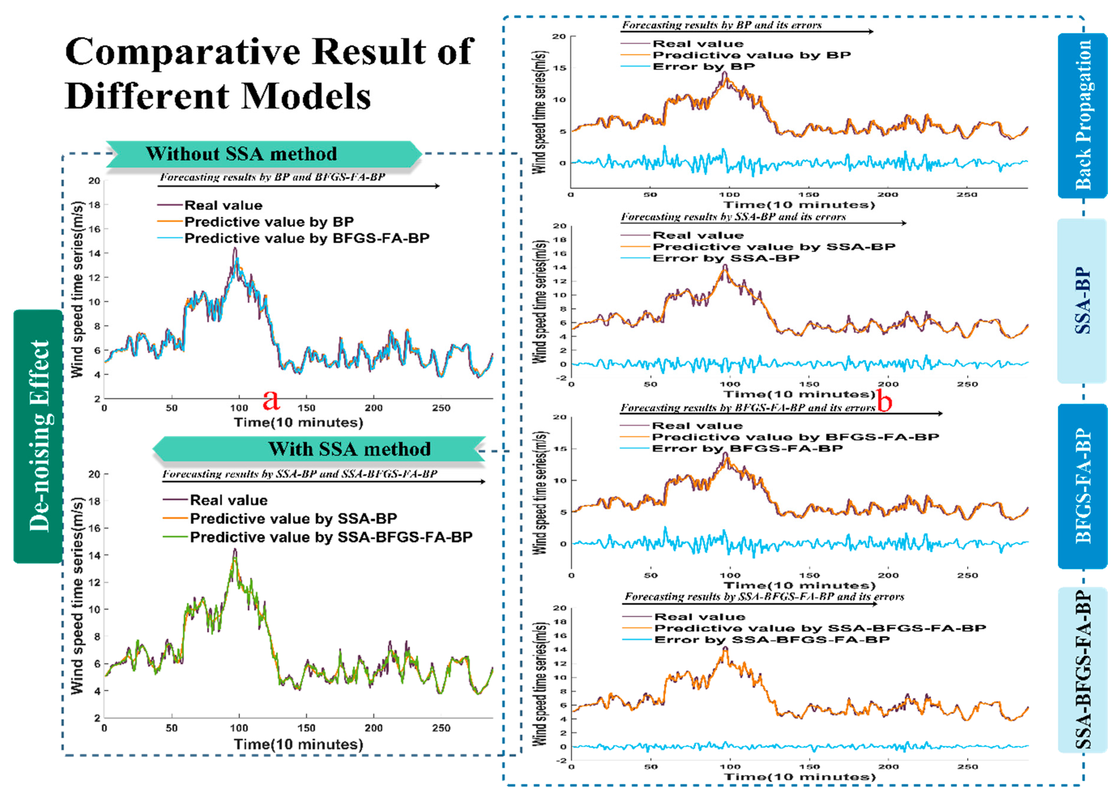
Figure 5.
The forecast results for wind speed collected from site 2 at 10-min intervals. (a) The forecast effect without SSA algorithm and with SSA algorithm; (b) The comparison between the forecast values and the raw data and their corresponding errors.
Figure 5.
The forecast results for wind speed collected from site 2 at 10-min intervals. (a) The forecast effect without SSA algorithm and with SSA algorithm; (b) The comparison between the forecast values and the raw data and their corresponding errors.

Figure 6.
The forecast results for wind speed collected from site 3 at 10-min intervals. (a) The forecast effect without SSA algorithm and with SSA algorithm; (b) The comparison between the forecast values and the raw data and their corresponding errors.
Figure 6.
The forecast results for wind speed collected from site 3 at 10-min intervals. (a) The forecast effect without SSA algorithm and with SSA algorithm; (b) The comparison between the forecast values and the raw data and their corresponding errors.

Table 1.
Summary of intelligent and hybrid forecasting methods and theoretical comparison of existing forecasting models. RBF: radial basis function; ENN: Elman neural network; WNN: Wavelet neural network; GA: genetic algorithm; BP: back propagation; FA: firefly algorithm; PSO: particle swarm optimization.
| Models | Variables | Date Set | Results | Advantages | Disadvantages | Ref. |
|---|---|---|---|---|---|---|
| RBF | Wind speed | March 2012 in Jiangsu, Ningxia and Yunnan, China | The proposed methods can provide higher quality prediction intervals than the conventional method. | Has a good local approximation and computer implementation is easy. | Has a low forecasting performance. | [40] |
| ENN | Wind speed | January 2010 to March 2011 in Gansu, China. | The proposed approach is an effective way to improve prediction accuracy. | Has a good fitting effect and can deal with nonlinear data. | Has a narrow forecasting scale. | [41] |
| WNN | Wind speed | 720 samplings in Inner Mongolia, China | The proposed model can be a robust method for wind speed forecasting. | Has a good forecasting performance and higher computational efficiency. | The model is unstable and highly dependent on time series. | [42] |
| Hybrid GA and BP | Wind speed | January 2011 in Inner Mongolia, China. | The method can improve both forecasting accuracy and computational efficiency. | The simulation method is easy to understand and combines with other methods. | It is easy to get into local optimum. | [43] |
| Hybrid FA/PSO Elman | Wind speed | January 2011 to November 2011 in Shandong, China. | The proposed model outperforms other comparative models in forecasting. | Has good adaptability, and can take advantage of other models. | The process of building models is relatively complex. | [44] |
Table 2.
The experimental set points of BP.
| Experimental Set Point | Default Value |
|---|---|
| The number of units in the input layer | 6 |
| The number of units in the hidden layer | 7 |
| The number of units in the output layer | 1 |
| The learning rate | 0.1 |
| The maximum training time | 1000 |
| Required accuracy of training | 0.00001 |
Table 3.
The experimental set points of FA.
| Experimental Set Point | FA |
|---|---|
| Maximum iteration | 1000 |
| Population size | 20 |
| Alpha | 0.25 |
| Beta | 0.2 |
| Gamma | 1 |
| Convergence tolerance | 0.00001 |
Table 4.
The metric equations.
| Error Index | Definition | Formula |
|---|---|---|
| MAE | The mean absolute error of T times predictive results | |
| RMSE | The root mean square error | |
| MAPE | The mean absolute percentage error |
Table 5.
The results of the hybrid model, ARIMA and SVM model at three sites.
| Model | Site 1 | Site 2 | Site 3 | ||||||
|---|---|---|---|---|---|---|---|---|---|
| MAE | RMSE | MAPE | MAE | RMSE | MAPE | MAE | RMSE | MAPE | |
| ARIMA | 0.5210 | 0.6832 | 7.9275 | 0.4496 | 0.5995 | 6.8094 | 0.5404 | 0.7606 | 10.4179 |
| SVM | 0.5069 | 0.6789 | 7.5806 | 0.4526 | 0.6118 | 6.8365 | 0.5379 | 0.7573 | 10.3284 |
| Hybrid model | 0.1849 | 0.2461 | 4.8496 | 0.2337 | 0.2465 | 4.5512 | 0.2407 | 0.2851 | 6.7548 |
Table 6.
The experimental parameters of singular spectrum analysis (SSA).
| Experimental Parameters | SSA |
|---|---|
| Embedding dimension | 50 |
| Components | 10 |
| Method of calculating the covariance matrix | Unbiased (N-K weighted) Biased (N-weighted or Yule-Walker) BK(Broomhead/King type estimate) |
Table 7.
MAE, RMSE, and MAPE of site 1 for each forecasting model.
| Numbers of Test | BP | BFGS-FA-BP | SSA-BP | SSA-BFGS-FA-BP | ||||||||
|---|---|---|---|---|---|---|---|---|---|---|---|---|
| MAE | RMSE | MAPE | MAE | RMSE | MAPE | MAE | RMSE | MAPE | MAE | RMSE | MAPE | |
| 1 | 0.5017 | 0.6789 | 7.6543 | 0.5113 | 0.6892 | 7.5143 | 0.3482 | 0.4643 | 5.2833 | 0.1835 | 0.2453 | 4.9052 |
| 2 | 0.5217 | 0.6871 | 7.7668 | 0.5145 | 0.6868 | 7.6611 | 0.3479 | 0.4632 | 5.2902 | 0.1853 | 0.2454 | 4.8152 |
| 3 | 0.5038 | 0.6769 | 8.2622 | 0.508 | 0.6758 | 7.5722 | 0.3487 | 0.4645 | 5.3063 | 0.1831 | 0.2461 | 4.7851 |
| 4 | 0.5064 | 0.6767 | 8.0176 | 0.5098 | 0.678 | 7.6388 | 0.3472 | 0.4633 | 5.2917 | 0.1833 | 0.246 | 4.0152 |
| 5 | 0.5364 | 0.6951 | 8.041 | 0.5225 | 0.6869 | 7.6698 | 0.3475 | 0.4638 | 5.292 | 0.1883 | 0.2462 | 4.8752 |
| 6 | 0.5118 | 0.6848 | 7.7139 | 0.5122 | 0.684 | 7.6718 | 0.3483 | 0.4636 | 5.302 | 0.1813 | 0.2465 | 4.6995 |
| 7 | 0.5051 | 0.6848 | 7.9229 | 0.5234 | 0.692 | 7.5886 | 0.3478 | 0.4636 | 5.2923 | 0.1873 | 0.2462 | 4.8905 |
| 8 | 0.5133 | 0.6827 | 7.9593 | 0.5121 | 0.6826 | 7.5832 | 0.3473 | 0.4637 | 5.303 | 0.1835 | 0.2461 | 4.7775 |
| 9 | 0.5243 | 0.6855 | 7.7893 | 0.5155 | 0.6805 | 7.6507 | 0.3474 | 0.4632 | 5.2966 | 0.1839 | 0.2462 | 4.9824 |
| 10 | 0.5161 | 0.6838 | 8.2 | 0.5068 | 0.6807 | 7.6527 | 0.3466 | 0.4631 | 5.2993 | 0.1983 | 0.2462 | 4.9867 |
| 11 | 0.5333 | 0.6941 | 7.6998 | 0.5109 | 0.6829 | 7.5984 | 0.348 | 0.4636 | 5.2924 | 0.1884 | 0.2461 | 4.2015 |
| 12 | 0.5091 | 0.6785 | 7.708 | 0.5121 | 0.6835 | 7.6684 | 0.3475 | 0.4637 | 5.2859 | 0.1823 | 0.246 | 4.2152 |
| 13 | 0.5277 | 0.6877 | 7.9615 | 0.5063 | 0.6757 | 7.5189 | 0.3467 | 0.4631 | 5.2933 | 0.1835 | 0.2459 | 4.5952 |
| 14 | 0.5106 | 0.6864 | 7.74 | 0.5123 | 0.6824 | 7.6302 | 0.3475 | 0.4634 | 5.2884 | 0.1833 | 0.2465 | 4.8951 |
| 15 | 0.5218 | 0.6858 | 8.1374 | 0.5042 | 0.6834 | 7.6242 | 0.3471 | 0.4633 | 5.2926 | 0.1803 | 0.2458 | 4.3895 |
| 16 | 0.5111 | 0.6874 | 7.7658 | 0.5027 | 0.6812 | 7.6604 | 0.3471 | 0.4631 | 5.3006 | 0.1893 | 0.2464 | 4.8679 |
| 17 | 0.5086 | 0.6832 | 7.6895 | 0.5117 | 0.6853 | 7.6 | 0.3481 | 0.4636 | 5.2913 | 0.1836 | 0.2462 | 4.2509 |
| 18 | 0.5078 | 0.6773 | 7.7802 | 0.5075 | 0.6767 | 7.6615 | 0.3469 | 0.4633 | 5.2944 | 0.1834 | 0.2463 | 4.5995 |
| 19 | 0.5199 | 0.6811 | 7.8523 | 0.508 | 0.6802 | 7.5538 | 0.3471 | 0.4633 | 5.3011 | 0.1813 | 0.2466 | 4.7655 |
| 20 | 0.515 | 0.6859 | 7.9596 | 0.501 | 0.6662 | 7.663 | 0.3474 | 0.4634 | 5.2851 | 0.1843 | 0.2457 | 4.4792 |
| Average value | 0.5153 | 0.6842 | 7.8811 | 0.5106 | 0.6817 | 7.6191 | 0.3475 | 0.4635 | 5.2941 | 0.1849 | 0.2461 | 4.8496 |
Table 8.
MAE, RMSE, and MAPE of site 2 for each forecasting model.
| Numbers of Test | BP | BFGS-FA-BP | SSA-BP | SSA-BFGS-FA-BP | ||||||||
|---|---|---|---|---|---|---|---|---|---|---|---|---|
| MAE | RMSE | MAPE | MAE | RMSE | MAPE | MAE | RMSE | MAPE | MAE | RMSE | MAPE | |
| 1 | 0.473 | 0.6309 | 7.0188 | 0.444 | 0.5972 | 6.6955 | 0.3272 | 0.426 | 4.9888 | 0.2327 | 0.2427 | 4.3499 |
| 2 | 0.4704 | 0.6253 | 7.0698 | 0.4447 | 0.608 | 6.6478 | 0.3268 | 0.4254 | 4.9841 | 0.2033 | 0.2343 | 4.45 |
| 3 | 0.4785 | 0.6279 | 7.0767 | 0.444 | 0.594 | 6.6344 | 0.3272 | 0.4261 | 4.9866 | 0.2433 | 0.2243 | 4.65 |
| 4 | 0.4688 | 0.6207 | 7.0969 | 0.4423 | 0.5955 | 6.6792 | 0.3272 | 0.4258 | 4.9942 | 0.2433 | 0.2543 | 4.7499 |
| 5 | 0.4563 | 0.6109 | 6.8203 | 0.4471 | 0.6016 | 6.6969 | 0.3286 | 0.428 | 5.0096 | 0.2533 | 0.3278 | 4.4995 |
| 6 | 0.468 | 0.6236 | 6.9768 | 0.445 | 0.5972 | 6.7103 | 0.3276 | 0.4268 | 4.994 | 0.2733 | 0.2043 | 4.5105 |
| 7 | 0.4767 | 0.6394 | 7.1899 | 0.4424 | 0.5932 | 6.6757 | 0.3282 | 0.4269 | 5.0038 | 0.2133 | 0.2427 | 4.992 |
| 8 | 0.4682 | 0.6276 | 6.9898 | 0.4519 | 0.6107 | 6.7899 | 0.3277 | 0.4266 | 4.998 | 0.2432 | 0.2333 | 4.3489 |
| 9 | 0.4848 | 0.6525 | 7.3656 | 0.4419 | 0.5975 | 6.6656 | 0.3272 | 0.4262 | 4.9893 | 0.2328 | 0.2554 | 4.4655 |
| 10 | 0.4608 | 0.6133 | 6.8227 | 0.4482 | 0.6016 | 6.7711 | 0.3275 | 0.4262 | 4.9952 | 0.2328 | 0.2412 | 4.651 |
| 11 | 0.462 | 0.6164 | 6.8987 | 0.4455 | 0.6022 | 6.7745 | 0.3272 | 0.4265 | 4.9918 | 0.2631 | 0.2943 | 4.8215 |
| 12 | 0.4547 | 0.6126 | 6.9756 | 0.4455 | 0.6025 | 6.721 | 0.3274 | 0.4265 | 4.996 | 0.2328 | 0.2342 | 4.3499 |
| 13 | 0.4592 | 0.612 | 6.8545 | 0.4439 | 0.598 | 6.6876 | 0.3276 | 0.4268 | 4.994 | 0.3026 | 0.2444 | 4.585 |
| 14 | 0.509 | 0.6582 | 7.4376 | 0.4444 | 0.6028 | 6.6422 | 0.3268 | 0.4258 | 4.9876 | 0.2533 | 0.2453 | 4.251 |
| 15 | 0.5148 | 0.6677 | 7.3453 | 0.4438 | 0.5961 | 6.7134 | 0.3269 | 0.4256 | 4.9842 | 0.2132 | 0.2433 | 4.815 |
| 16 | 0.4474 | 0.5996 | 7.0924 | 0.4467 | 0.5991 | 6.7905 | 0.328 | 0.4274 | 4.9991 | 0.2031 | 0.2121 | 4.2501 |
| 17 | 0.4674 | 0.6244 | 6.9551 | 0.4426 | 0.5946 | 6.679 | 0.3276 | 0.427 | 4.9964 | 0.2234 | 0.2543 | 4.495 |
| 18 | 0.4688 | 0.6245 | 7.0109 | 0.441 | 0.5963 | 6.6643 | 0.3274 | 0.4261 | 4.9922 | 0.2132 | 0.2314 | 4.625 |
| 19 | 0.4704 | 0.6391 | 7.0898 | 0.4427 | 0.5936 | 6.6678 | 0.3265 | 0.4252 | 4.9808 | 0.1935 | 0.2333 | 4.4635 |
| 20 | 0.4685 | 0.615 | 7.1212 | 0.444 | 0.5965 | 6.6865 | 0.3277 | 0.4272 | 5.0004 | 0.2032 | 0.2768 | 4.7011 |
| Average value | 0.4714 | 0.6271 | 7.0604 | 0.4446 | 0.5989 | 6.6997 | 0.3274 | 0.4264 | 4.9933 | 0.2337 | 0.2465 | 4.5512 |
Table 9.
MAE, RMSE, and MAPE of site 3 for each forecasting model.
| Numbers of test | BP | BFGS-FA-BP | SSA-BP | SSA-BFGS-FA-BP | ||||||||
|---|---|---|---|---|---|---|---|---|---|---|---|---|
| MAE | RMSE | MAPE | MAE | RMSE | MAPE | MAE | RMSE | MAPE | MAE | RMSE | MAPE | |
| 1 | 0.5404 | 0.7577 | 10.7941 | 0.5488 | 0.7665 | 10.4888 | 0.3887 | 0.5128 | 7.5209 | 0.2389 | 0.2851 | 6.752 |
| 2 | 0.5612 | 0.7752 | 10.9005 | 0.5623 | 0.7899 | 10.4192 | 0.3891 | 0.5143 | 7.5248 | 0.2389 | 0.2905 | 6.7538 |
| 3 | 0.5503 | 0.7679 | 10.784 | 0.5426 | 0.7681 | 10.5803 | 0.3905 | 0.5148 | 7.5595 | 0.2439 | 0.3051 | 7.0753 |
| 4 | 0.5519 | 0.7718 | 11.1111 | 0.5472 | 0.7707 | 10.6574 | 0.3882 | 0.5124 | 7.5094 | 0.2139 | 0.2885 | 6.6716 |
| 5 | 0.5509 | 0.7757 | 10.7029 | 0.5475 | 0.7694 | 10.6845 | 0.3902 | 0.5152 | 7.5699 | 0.2563 | 0.2768 | 6.9975 |
| 6 | 0.5518 | 0.7843 | 10.7331 | 0.5485 | 0.7601 | 10.6767 | 0.3888 | 0.5132 | 7.5312 | 0.2609 | 0.2905 | 7.1275 |
| 7 | 0.552 | 0.7628 | 10.8619 | 0.5645 | 0.7787 | 10.4793 | 0.3893 | 0.5142 | 7.5439 | 0.2389 | 0.279 | 6.8768 |
| 8 | 0.5561 | 0.7801 | 10.7375 | 0.5531 | 0.772 | 10.6667 | 0.3893 | 0.5135 | 7.5346 | 0.2204 | 0.2676 | 6.6675 |
| 9 | 0.553 | 0.7762 | 11.4947 | 0.534 | 0.7523 | 10.6886 | 0.3906 | 0.5154 | 7.5668 | 0.2539 | 0.2595 | 6.9075 |
| 10 | 0.5407 | 0.7588 | 10.6916 | 0.5515 | 0.7753 | 10.4897 | 0.3913 | 0.5158 | 7.6121 | 0.2339 | 0.3151 | 6.1558 |
| 11 | 0.5583 | 0.7745 | 10.9143 | 0.5571 | 0.7755 | 10.5834 | 0.3888 | 0.5135 | 7.5325 | 0.239 | 0.3005 | 6.8776 |
| 12 | 0.5615 | 0.7698 | 10.8 | 0.5462 | 0.7687 | 10.307 | 0.3884 | 0.5127 | 7.5142 | 0.2432 | 0.2982 | 6.6275 |
| 13 | 0.5447 | 0.7655 | 10.9335 | 0.5554 | 0.7754 | 10.5456 | 0.3897 | 0.514 | 7.526 | 0.2733 | 0.2775 | 6.8098 |
| 14 | 0.5491 | 0.7628 | 10.7102 | 0.5522 | 0.7697 | 10.5567 | 0.3915 | 0.5157 | 7.586 | 0.214 | 0.2591 | 6.4725 |
| 15 | 0.5466 | 0.77 | 10.8156 | 0.5456 | 0.7632 | 10.5918 | 0.3884 | 0.5134 | 7.537 | 0.2399 | 0.2835 | 6.7357 |
| 16 | 0.5415 | 0.7591 | 10.7132 | 0.549 | 0.7696 | 10.5576 | 0.3896 | 0.5142 | 7.5376 | 0.2238 | 0.2499 | 7.1752 |
| 17 | 0.5526 | 0.7702 | 10.9634 | 0.5483 | 0.7623 | 10.4912 | 0.3902 | 0.5151 | 7.5778 | 0.2546 | 0.29 | 6.3975 |
| 18 | 0.5608 | 0.7855 | 10.9059 | 0.5423 | 0.7615 | 10.4807 | 0.389 | 0.5124 | 7.5297 | 0.2434 | 0.2945 | 6.7595 |
| 19 | 0.5486 | 0.7667 | 11.2402 | 0.5378 | 0.7585 | 10.6654 | 0.3885 | 0.5126 | 7.5293 | 0.2386 | 0.2795 | 6.9808 |
| 20 | 0.5426 | 0.7708 | 10.9645 | 0.5437 | 0.7586 | 10.5158 | 0.3874 | 0.5122 | 7.4898 | 0.2444 | 0.3125 | 6.2753 |
| Average value | 0.5507 | 0.7703 | 10.8886 | 0.5489 | 0.7683 | 10.5563 | 0.3894 | 0.5139 | 7.5417 | 0.2407 | 0.2851 | 6.7548 |
Table 10.
MAE, RMSE, and MAPE of four seasons and various iterations in one site for each forecasting model.
Table 10.
MAE, RMSE, and MAPE of four seasons and various iterations in one site for each forecasting model.
| Model | Error Index | Season | Iteration | ||||||
|---|---|---|---|---|---|---|---|---|---|
| Spring | Summer | Autumn | Winter | One | Three | Six | Twelve | ||
| BP | MAE | 0.5153 | 0.5975 | 0.4804 | 0.6708 | 0.5153 | 0.7955 | 1.0541 | 1.2740 |
| RMSE | 0.6842 | 0.8103 | 0.6054 | 1.0172 | 0.6842 | 1.0229 | 1.3421 | 1.6878 | |
| MAPE | 7.8811 | 9.5102 | 13.7179 | 7.4235 | 7.8811 | 12.4853 | 16.7727 | 20.3831 | |
| BFGS-FA-BP | MAE | 0.5106 | 0.6049 | 0.4629 | 0.5272 | 0.5106 | 0.7745 | 1.0051 | 1.3240 |
| RMSE | 0.6817 | 0.7996 | 0.5854 | 0.6651 | 0.6817 | 1.0064 | 1.2991 | 1.7399 | |
| MAPE | 7.6191 | 9.2133 | 13.1582 | 6.1367 | 7.6191 | 12.0691 | 16.1433 | 21.2589 | |
| SSA-BP | MAE | 0.3475 | 0.4486 | 0.3368 | 0.3625 | 0.3475 | 0.3651 | 0.6742 | 1.3673 |
| RMSE | 0.4635 | 0.5659 | 0.4243 | 0.4544 | 0.4635 | 0.4824 | 0.8456 | 1.7684 | |
| MAPE | 5.2941 | 7.1654 | 9.9706 | 4.2700 | 5.2941 | 5.4943 | 10.6671 | 21.2998 | |
| SSA- BFGS-FA-BP | MAE | 0.1849 | 0.3875 | 0.2863 | 0.3159 | 0.1849 | 0.3354 | 0.6370 | 1.4349 |
| RMSE | 0.2461 | 0.4961 | 0.3941 | 0.4018 | 0.2461 | 0.4389 | 0.8154 | 1.8355 | |
| MAPE | 4.8496 | 5.2463 | 7.5297 | 3.4269 | 4.8496 | 4.8671 | 9.9499 | 22.5317 | |
Table 11.
MAE, RMSE, and MAPE of various intervals in one site for each forecasting model.
| Time (minutes) | Model error | BP | BFGS-FA-BP | SSA-BP | SSA-BFGS-FA-BP |
|---|---|---|---|---|---|
| 10 | MAE | 0.5153 | 0.5106 | 0.3475 | 0.1849 |
| RMSE | 0.6842 | 0.6817 | 0.4635 | 0.2461 | |
| MAPE | 7.8811 | 7.6191 | 5.2941 | 4.8496 | |
| 30 | MAE | 0.9769 | 0.9444 | 0.6193 | 0.5854 |
| RMSE | 1.3655 | 1.2808 | 0.8087 | 0.7426 | |
| MAPE | 9.9414 | 9.4053 | 6.6134 | 5.4780 | |
| 60 | MAE | 0.9253 | 0.8890 | 0.6244 | 0.6043 |
| RMSE | 1.1464 | 1.1116 | 0.7881 | 0.7392 | |
| MAPE | 28.3766 | 26.0956 | 19.1245 | 17.4441 |
Table 12.
Results of the DM test and operational time (s).
| Performance Metric | Compared Model | Average Value |
|---|---|---|
| DM-test | BP | 8.1064 * |
| SSA-BP | 8.0468 * | |
| BFGS-FA-BP | 8.1696 * | |
| Operational time | BP | 0.3 |
| SSA-BP | 0.6 | |
| BFGS-FA-BP | 490.3 | |
| Hybrid model | 157.1 |
Note: * Indicates the 1% significance level.
Table 13.
The DRP of MAPE of the proposed model and comparison models.
| Cases | DRP of MAPE (%) | |||
|---|---|---|---|---|
| ENN | WNN | PSO/FA Elman | Proposed Model | |
| case 1 | 15.6250 | 10.2506 | 13.9158 | 38.4654 |
| case 2 | 24.0000 | 32.1063 | 12.7855 | 35.5391 |
| case 3 | 47.8261 | - | 15.4897 | 37.9645 |
| case 4 | 35.2941 | - | - | - |
Table 14.
Comparison results of three observation sites with different time intervals.
| Observation Sites | 10-min | 30-min | 60-min |
|---|---|---|---|
| Site 1 | 4.8496 | 5.4780 | 17.4441 |
| Site 2 | 4.5512 | 9.8730 | 14.6964 |
| Site 3 | 6.7548 | 12.9558 | 18.1605 |
© 2017 by the authors. Licensee MDPI, Basel, Switzerland. This article is an open access article distributed under the terms and conditions of the Creative Commons Attribution (CC BY) license (http://creativecommons.org/licenses/by/4.0/).
Share and Cite
MDPI and ACS Style
Jiang, P.; Wang, Z.; Zhang, K.; Yang, W. An Innovative Hybrid Model Based on Data Pre-Processing and Modified Optimization Algorithm and Its Application in Wind Speed Forecasting. Energies 2017, 10, 954. https://doi.org/10.3390/en10070954
AMA Style
Jiang P, Wang Z, Zhang K, Yang W. An Innovative Hybrid Model Based on Data Pre-Processing and Modified Optimization Algorithm and Its Application in Wind Speed Forecasting. Energies. 2017; 10(7):954. https://doi.org/10.3390/en10070954
Chicago/Turabian StyleJiang, Ping, Zeng Wang, Kequan Zhang, and Wendong Yang. 2017. "An Innovative Hybrid Model Based on Data Pre-Processing and Modified Optimization Algorithm and Its Application in Wind Speed Forecasting" Energies 10, no. 7: 954. https://doi.org/10.3390/en10070954
Note that from the first issue of 2016, this journal uses article numbers instead of page numbers. See further details here.