
Fault Diagnosis of On-Load Tap-Changer Based on Variational Mode Decomposition and Relevance Vector Machine


1
School of Electrical Engineering, Shandong University, Jinan 250061, China
2
Shandong Provincial Key Lab of UHV Transmission Technology and Equipment, Jinan 250061, China
*
Author to whom correspondence should be addressed.
Energies 2017, 10(7), 946; https://doi.org/10.3390/en10070946
Submission received: 30 March 2017
/
Revised: 21 June 2017
/
Accepted: 4 July 2017
/
Published: 8 July 2017
(This article belongs to the Special Issue Selected Papers from 2016 IEEE International Conference on High Voltage Engineering (ICHVE 2016))
Abstract
:In order to improve the intelligent diagnosis level of an on-load tap-changer’s (OLTC) mechanical condition, a feature extraction method based on variational mode decomposition (VMD) and weight divergence was proposed. The harmony search (HS) algorithm was used to optimize the parameter selection of the relevance vector machine (RVM). Firstly, the OLTC vibration signal was decomposed into a series of finite-bandwidth intrinsic mode function (IMF) by VMD under different working conditions. The weight divergence was extracted to characterize the complexity of the vibration signal. Then, weight divergence was used as training and test samples of the harmony search optimization-relevance vector machine (HS-RVM). The experimental results suggested that the proposed integrated model has high fault diagnosis accuracy. This model can accurately extract the characteristics of the mechanical condition, and provide a reference for the practical OLTC intelligent fault diagnosis.
1. Introduction
Power transformers are important power transformation equipment, and their stable operation is the premise of power system security. However, the on-load tap-changer (OLTC) has a high failure rate, which has been a major threat to the health of transformers. According to statistics [1], OLTC failure, accounting for more than 27% of the total transformer failure, is the main cause of transformer failure, and the fault type is mostly mechanical failure, such as the operating mechanism jamming, gear slipping, refusal to operate, and so on. Therefore, it has important theoretical and practical significance to improve the on-line monitoring capability of OLTC mechanical status by seeking a more efficient and suitable intelligent diagnosis algorithm.
In recent years, there have been a large number of experts and scholars engaged in OLTC on-line monitoring and fault diagnosis. With the vibration, motor current, motor rotation angle, thermal noise and arcing signals as preselected inputs, a variety of integrated fault diagnosis strategies for OLTC have been proposed [2,3,4,5]. However, the disposals of vibration signals are the core of the integrated fault diagnosis strategy, and the studies on the processing of OLTC vibration signals are still imperfect. Consequently, finding a vibration signal processing algorithm, the key to improving the OLTC on-line monitoring capability, was the focus of scholars’ research [6,7,8]. The OLTC vibration signals are analyzed in the time domain by employing different wavelet analysis methods in the literature [9,10,11], but the traditional time–frequency analysis method is not suitable for non-stationary signals. Based on empirical mode decomposition (EMD) and the Hilbert transform, the vibration signal is studied in the literature [12]. However, the signal processing of the EMD algorithm has the phenomenon of mode mixing, which leads to inaccurate results. Hong presents an OLTC fault diagnosis method based on ensemble empirical mode decomposition (EEMD), which abates the phenomenon of the mode mixing in the EMD algorithm [13]. Nevertheless, the EEMD algorithm suppresses the mode aliasing by adding white noise. This method requires many EMD operations, resulting in a significant increase in computation.
Variational mode decomposition (VMD) is a new adaptive and multi-resolution decomposition technique; it not only retains the adaptive ability of EMD, but also avoids the problem of the mode mixing. Compared with the EEMD algorithm, the VMD algorithm completely eliminates the problem of modal aliasing and has small amount of computation [14].
A relevance vector machine (RVM) has the advantages of a support vector machine (SVM), while breaking through the limitations of SVM. RVM, avoiding the complex parameter setting problem, has better generalization performance and faster fault classification [15].
In summary, this paper presents an OLTC mechanical state diagnosis method based on VMD-weight divergence and harmony search optimization-relevance vector machine (HS-RVM). First, the OLTC vibration signal is decomposed into a series of finite-bandwidth intrinsic mode functions (IMF) by VMD. Next, the Kullback-Leibler divergence (K-L divergence) of the IMF and the original vibration signal is calculated, and then the weight divergence is used to characterize the complexity of the vibration signal. According to the experiment, the RVM multi-classification model is established, and the kernel function parameter of the RVM is optimized by the harmony search algorithm, which can improve the classification accuracy of the RVM. Both the theoretical analysis and experimental study have verified that the proposed fault diagnosis methodology is feasible and effective.
2. Variational Mode Decomposition-Weight Divergence
2.1. The Principle of Variational Mode Decomposition
The key of VMD signal processing is to solve the variational problem. Firstly, a variational model with constraints is constructed, and then the optimal solution of the model is searched to realize the adaptive separation of signals [16].
Assuming a given input signal y, the y is decomposed into K intrinsic mode function , k = 1, 2, …, K:
In Equation (1), is the instantaneous amplitude of , , and is the instantaneous frequency of .
Suppose that any has a definite center frequency and a finite bandwidth, the variational problem is to seek K intrinsic mode functions under constraint conditions.
There are two constraints:
- (1)
- The sum of modes is equal to the input signal.
- (2)
- The sum of the estimated bandwidth of the intrinsic mode functions is the smallest.
The variational questions with constraints are as follows:
In order to obtain the optimal solution of the variational problem, the second penalty factor α and the Lagrange multiplication operator λ(t) are introduced. The problem is transformed into a variational problem with no constraints, as shown in Equation (3):
The multiplication operator alternating direction method is used to solve the variational problem. Update , and to find the saddle point of Equation (3). The expression of is:
Equation (4) is converted to the frequency domain by using the Fourier equidistant transformation. The problem of the central frequency is extended to the frequency domain. The update method of the center frequency is obtained and the update of the λ is completed. Update expressions are as follows:
According to the above analysis, the solution of the variational problem can be simplified as follows [17]:
- (1)
- Initialize , , , and .
- (2)
- and are obtained according to Equations (5) and (6).
- (3)
- Updating Lagrange multipliers according to Equation (7).
- (4)
- Given discriminant accuracy e > 0. If Equation (8) is satisfied, the iteration of the algorithm will be stopped, otherwise return to Step 2.
2.2. The Principle of Weight Divergence
In order to continue to discover the fault information that is contained in the OLTC vibration signal, the concept of weight divergence is put forward on the basis of variational mode decomposition. The weight divergence consists of the weight coefficient and the K-L divergence.
K-L divergence is also called relative entropy, which can be used to characterize the difference between the two signals. The larger the divergence value, the larger the difference between the two signals. Therefore, the K-L divergence was introduced to measure the difference between the IMF and the original signal.
The K-L divergence principle and the solving process are described in the literature [18,19]. The solution of K-L divergence is simplified as follows:
- (1)
- Given the OLTC original vibration signal X = {x1, x2, …, xn} and IMF component Y = {y1, y2, …, yn}. The probability distribution function of the two signals is assumed to be p(x) and q(y).
- (2)
- The kernel density estimation of probability distribution function p(x) is given by Equation (9). Similarly, q(y) can be obtained.where k[*] is a Gaussian kernel function; h is a smoothing parameter.
- (3)
- Calculate the K-L distance of two signals by Equation (10):
- (4)
- Finally, the K-L divergence is obtained by the Equation (11):
The IMF component Y = {y1, y2, …, yn} corresponds to a certain main frequency. The reciprocal of the 1/104 of the IMF component is defined as the weight coefficient, and the weight coefficient is multiplied by the K-L divergence to obtain the weight divergence. Weight divergence, which reveals the distribution of the frequency in the signal, is an important criterion for detecting the operating state of the OLTC.
3. Harmony Search Algorithm for Optimization of Multi-Classification Relevance Vector Machine
3.1. The Principle of Relevance Vector Machine
Given a training sample set , , classification number [20]. The output function of RVM is:
where is the kernel function, and is the coefficient.
The relationship between and is as shown in Equation (13):
In Equation (13), εn is noise that obeys the Gaussian distribution.
The likelihood estimation function of the whole sample can be expressed as shown in Equation (14):
In the process of maximizing Equation (14), the maximum likelihood method is used to find w and . In order to prevent the phenomenon of over learning, the Gaussian prior probability distribution is defined for the weight w to constrain the parameters:
In Equation (15), α is an N + 1 dimensional hyper parameter. In this way, the solution of w is transformed into the solution of α. When α tends to infinity, w tends to 0.
3.2. The Model of Multi-Classification Relevance Vector Machine
Compared with the traditional support vector machine, the relevance vector machine has unique advantages. On the one hand, it avoids the problem of complex parameter setting; on the other hand, its solution has a stronger sparseness. The traditional SVM method can only realize the qualitative diagnosis of samples. RVM is able to quantitatively describe the diagnosis by Equation (13), and the diagnostic results are more practical. However, RVM belongs to the binary classifier, and can only output the probability of the two classification problems. OLTC fault classification belongs to the multi-classification problem. Therefore, it is necessary to carry out the multi-classification extension of RVM. In this paper, the binary tree model is used to solve the problem of RVM extension. According to the experiments, the multi-classification model of OLTC mechanical failure is established as shown in Figure 1. With the subsequent experiments, this model can be extended to achieve greater classification of the OLTC fault. In Figure 1, RVM1 classifier separates normal and fault status, where 0 indicates a normal condition, while 1 indicates the fault condition; the RVM2 classifier separates the jam fault and looseness fault, where 0 indicates the jam fault, while 1 indicates the looseness fault; the RVM3 classifier separates the main spring looseness and the main contact looseness, where 0 indicates the main spring looseness, while 1 indicates main contact looseness.
3.3. Harmony Search Algorithm
The harmony search algorithm is proposed based on the principle of musical performance. This algorithm has a strong global search ability and avoids the complex parameter setting problem. In many optimization problems, the performance of HS is better than genetic algorithms (GA) and simulated annealing (SA) algorithms [21,22]. In this paper, HS is used to optimize the kernel function parameter selection of the RVM to improve the classification accuracy of the OLTC classification model.
3.4. Optimization of Relevance Vector Machine by the Harmony Search Algorithm
The selection of kernel function parameters of the relevance vector machine are optimized by HS. The purpose is to choose the best kernel function parameters so that the relevance vector machine has high accuracy of fault classification [23,24]. A Gaussian kernel function is selected as the kernel function of the relevance vector machine, and the optimization process is as follows:
- (1)
- Define the fitness function and harmony dimension. The objective is to optimize the kernel function parameters of RVM1, RVM2, and RVM3. Therefore, the average value of the classification accuracy of the three RVM is defined as the fitness function, and the harmony dimension is set to 3.
- (2)
- Initialize parameters. Parameters that need to be initialized include: harmony memory (HM), harmony memory size (HMS), harmony memory considering rate (HMCR), pitch adjusting rate (PAR), bandwidth (bw), and termination criterion.
- (3)
- Initialize the HM. Generate HMS harmonies, which constitute the initial HM. Calculate the fitness value of each individual in the HM by calling the relevance vector machine.
- (4)
- Generate a new harmony. If rand1 < HMCR, an individual is selected from HM by Equation (16):Adjust the selected individuals by Equation (17); If rand1 < HMCR is not met, generate a new solution in the scope of variables:
- (5)
- Update HM. Calculate the fitness of the new solution. The HM is updated according to the following formula:
- (6)
- Termination criterion judgment. If the termination criterion is satisfied, the algorithm stops running. Otherwise, the algorithm continues to execute from step 3.
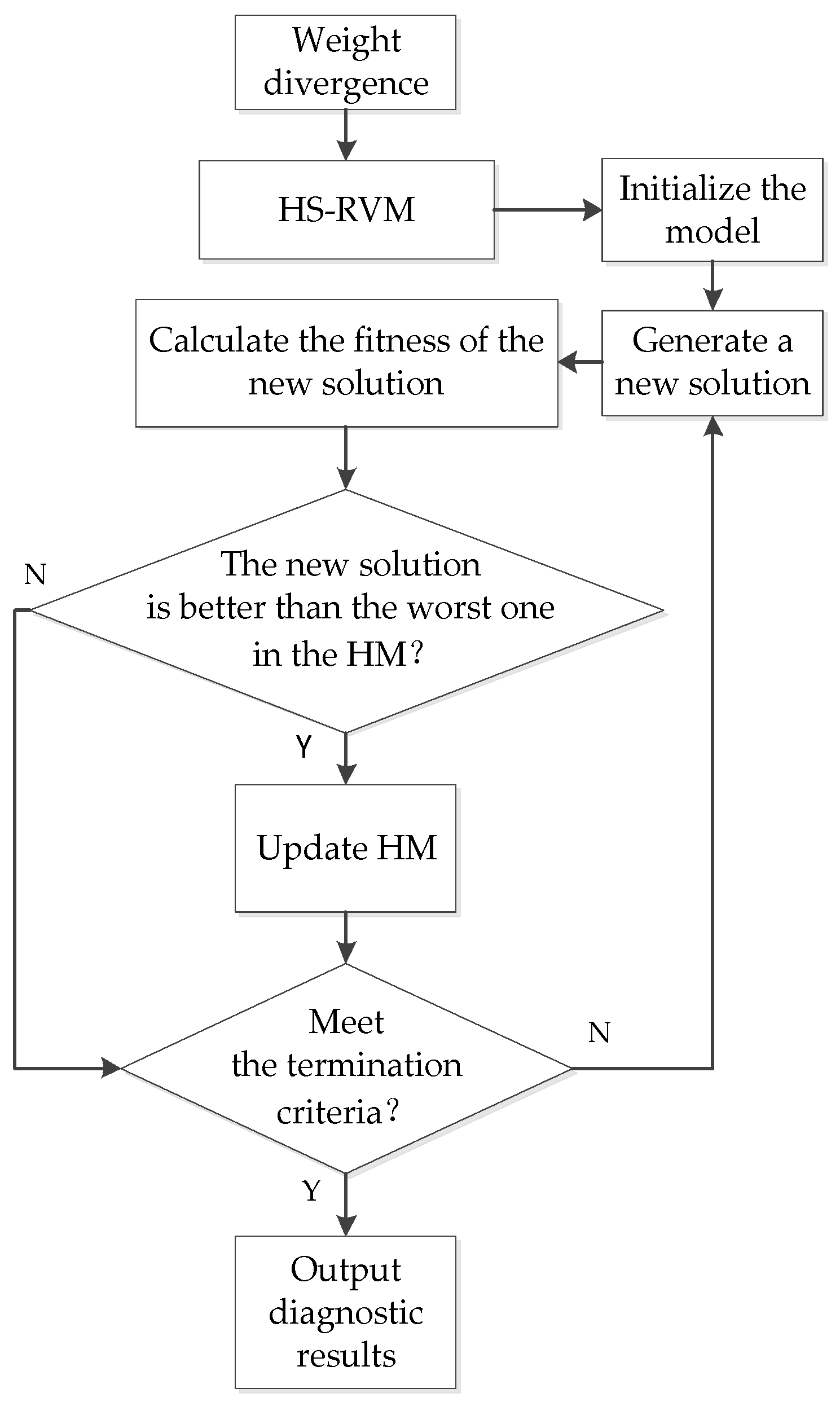
The algorithm flow of HS-RVM model is shown in Figure 2.
4. Experiment and Data Analysis
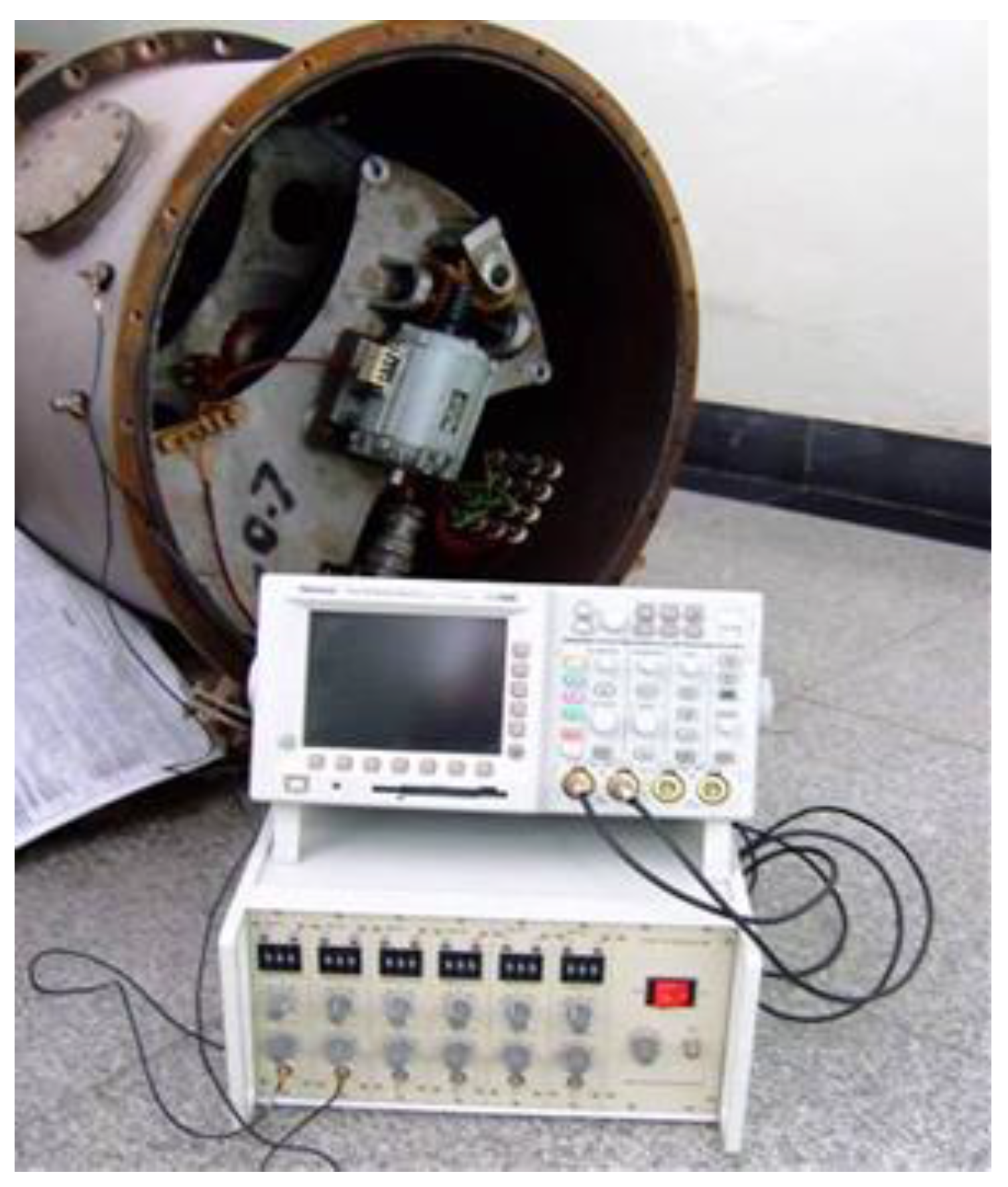
In the laboratory, a simulation experiment is carried out for a comprehensive-type OLTC by using the piezoelectric acceleration sensor, a charge amplifier, and a Tektronix oscilloscope. Information regarding the experimental equipment is shown in Table 1. The OLTC vibration test in the laboratory is shown in Figure 3.
In this paper, three types of faults, including a mechanism jam, main spring looseness, and main contact looseness, are simulated. Loosening the fixing screw of the main contact to simulate the main contact looseness fault; one of the two main springs is disconnected to simulate the main spring looseness fault; and the simulation of the jam fault is to tie a piece of wire into the instantaneous dial, which affects the bite of the dial and the grooved wheel. The sampling frequency is set to 50 kHz during the experiment.
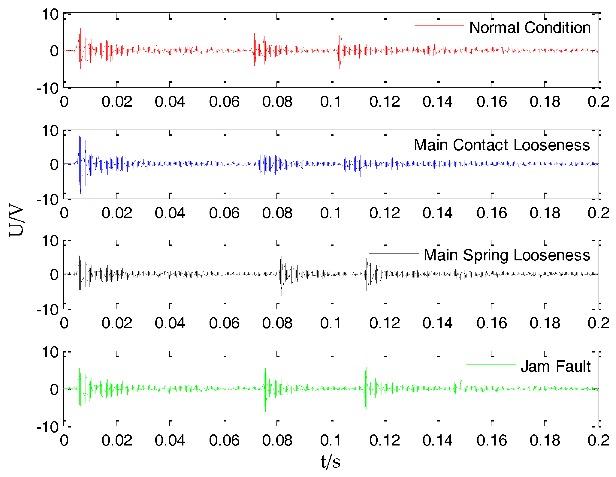
The mechanical vibration signal waveform of OLTC operation is obtained under the four conditions of normal, main spring looseness, main contact looseness and mechanism jam. In this paper, 85 sets of experimental data of OLTC vibration signal are selected. The data of the main spring looseness comprise of 24 groups, and the data under the mechanism jam comprise 21 groups. The data under normal conditions comprise 20 groups, and the fault of the main contact is under the looseness condition, which are the same as the 20 groups.
Four groups of typical vibration signals under different operating conditions are shown in Figure 4.
4.1. The Decomposition Process of Variational Mode Decomposition
The main contact looseness signal in Figure 4 is decomposed to demonstrate the VMD process. The original signal time–frequency diagram is shown in Figure 5.
The decomposition level K is identified by observing the center frequency and amplitude of the IMF component. Different K values are used to decompose the signal to obtain the stationary signal. Then, the center frequency of the IMF component and the corresponding FFT amplitude are read, and the results are shown in Table 2.
As can be seen from Table 2, when the decomposition level K = 4, the center frequencies of IMF3 and IMF4 are too close, which is considered as the phenomenon of over decomposition. When the decomposition level K = 5, not only the center frequencies are too close, but the amplitude of IMF5 is too low. Therefore, the decomposition level K = 3 is selected in this paper. We set the bandwidth constraint α to 2000 and the fidelity to 0.3.
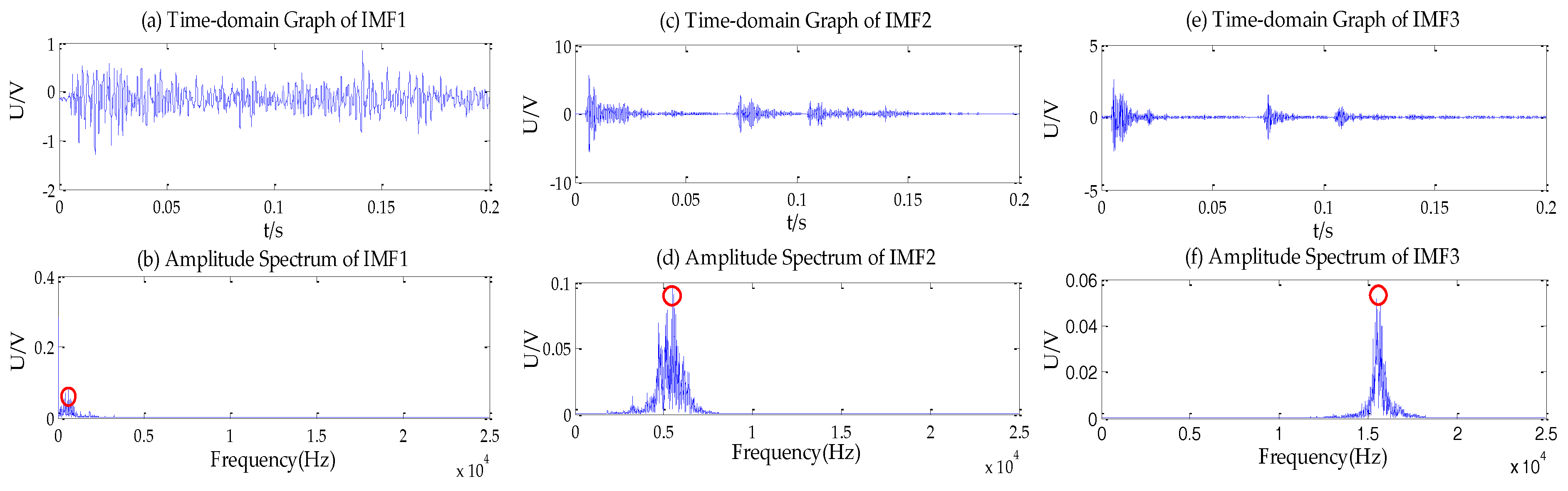
The results of decomposition are shown in Figure 6.
As shown in Figure 6, the three prominent peaks in Figure 5b are adaptively separated, and there is only one dominant frequency in the spectrum analysis of the IMF.
The IMF components are reconstructed as shown in Figure 7. It can be seen from the figure that the error between the reconstructed signal and the original signal is small. Thus, the decomposition process is in accordance with the positive expectations.
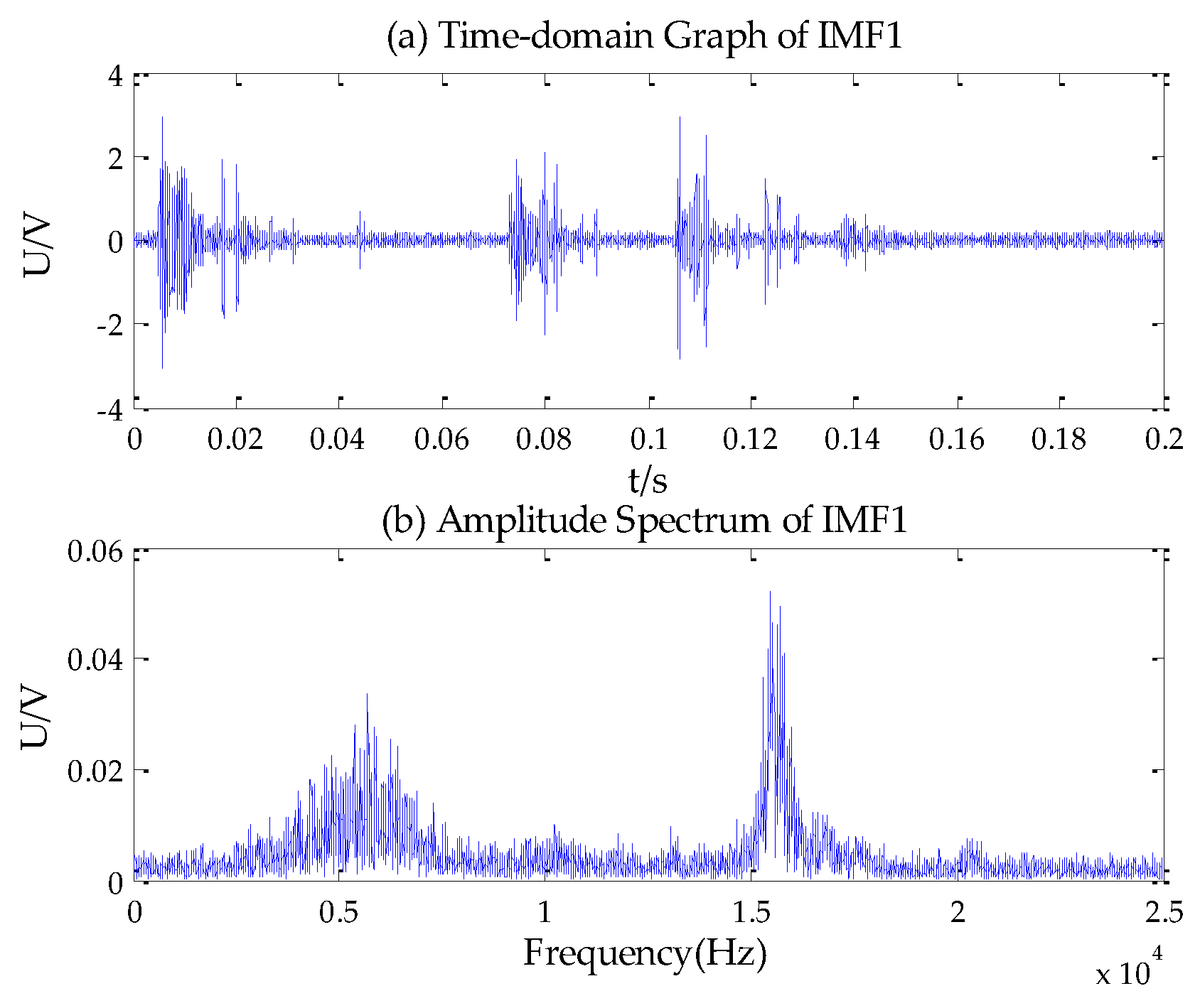
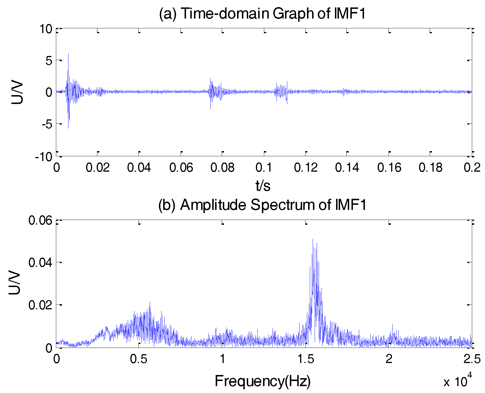
In order to illustrate the limitations of EMD and EEMD in the vibration signal processing of OLTC, the data in Figure 5a is decomposed by EMD and EEMD, respectively. The time–frequency diagrams of IMF1 obtained by EMD and EEMD are shown in Figure 8 and Figure 9 separately.
As can be seen from Figure 8b, the phenomenon of mode mixing exists in the result of EMD. There is no unique center frequency in the spectrum of IMF1, which contains a wide range of frequencies. The phenomenon of modal aliasing is suppressed in Figure 9, while it is not completely eliminated.
The comprehensive comparison of three algorithms is given in Table 3. Compared with EMD, there is no modal aliasing in VMD. Meanwhile, the operation time of VMD is shorter than EEMD. Therefore, the VMD algorithm is more suitable for the analysis of OLTC mechanical vibration signals.
4.2. The Analysis of Weight Divergence
In order to reflect the difference in the frequency distribution, the method of weight divergence is proposed to further extract the characteristics of the OLTC vibration signal. Firstly, the K-L divergence of each IMF and the original signal is calculated, which can represent the components of each frequency signal in the original signal. Then K-L divergence multiplied by the weight coefficient (i.e., 104 multiplied by the reciprocal of the main frequency of the IMF component).
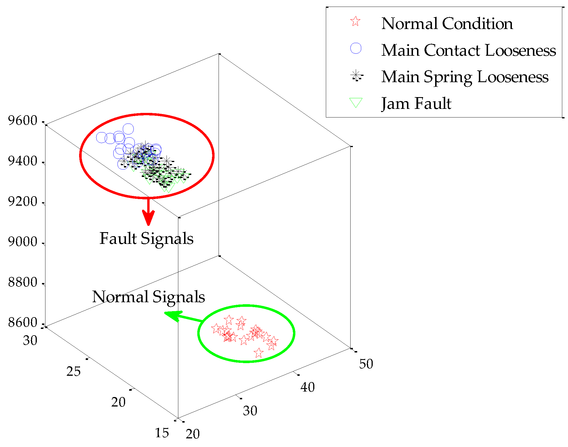
The distributions of 85 groups’ weight divergence of the OLTC vibration signal are shown in Figure 10.
It can be seen from Figure 10 that the weight divergence of the normal signal and the fault signal are significantly different. For the medium and low frequency signals, the main component is the normal condition signal, thus, the normal signal’s weight divergence of IMF1 and IMF2 are smaller than the fault, while the situations of high-frequency part are just the opposite. At the same time, there is a consistency between the weight divergences of three kinds of different fault types. In conclusion, the VMD-weight divergence model can better characterize the distribution of signals in different frequency bands, and it is easy to distinguish the fault signal from the normal one, while the distinction between the different fault signals is not obvious.
4.3. The Analysis of Harmony Search—Relevance Vector Machine
The 85 groups of weight divergence are used as the input of the classification model. The selections of the training set and test set are shown in Table 4.
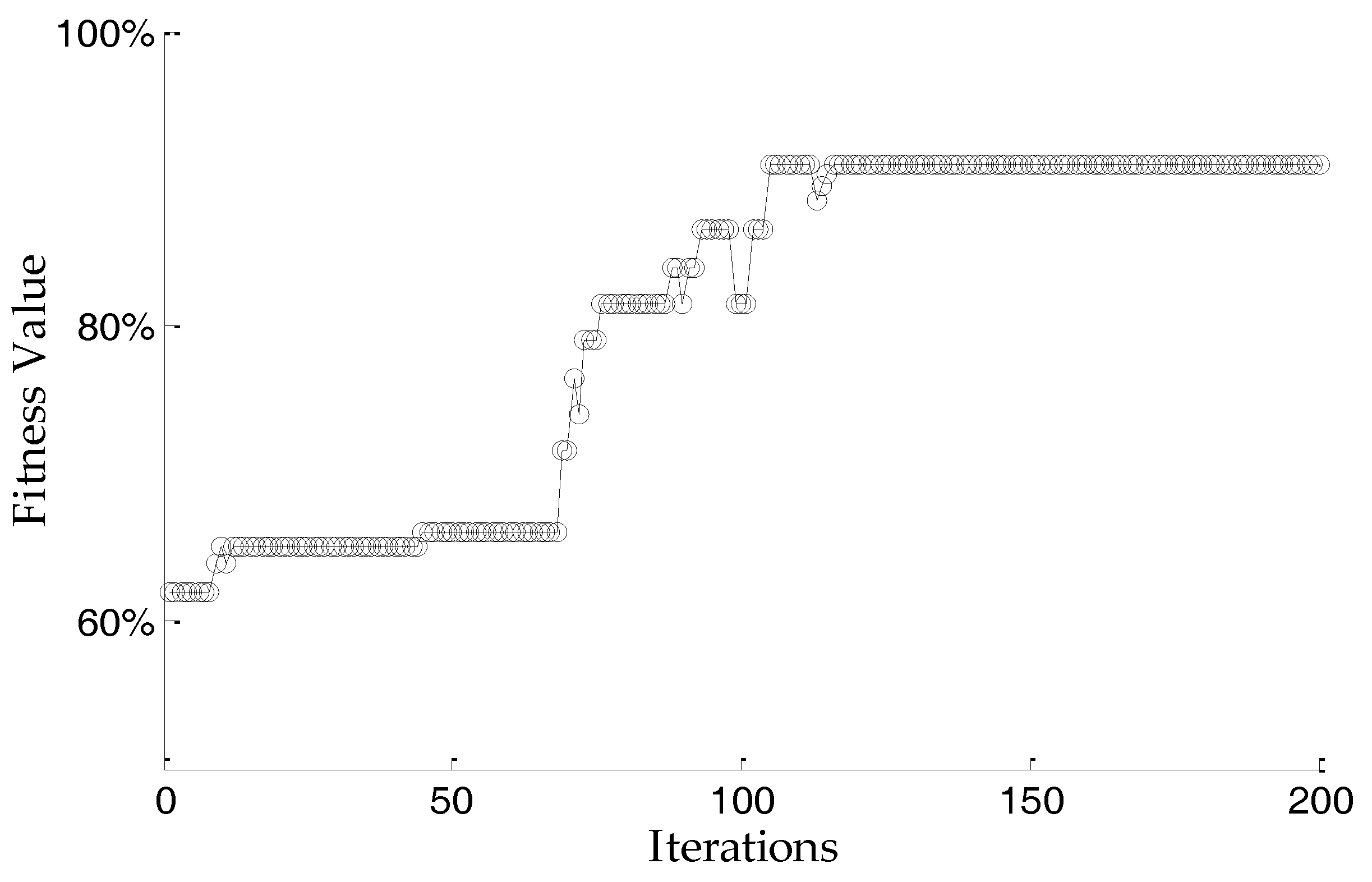
Using the HS-RVM model to diagnose the training set and test set, the parameters are set as follows: HM = 20, HMCR = 0.9, PARmin = 0.4, PARmax = 0.9, bwmin = 0.0001, bwmax = 1, Tmax = 200. The results are shown in Table 5, and the fitness curve is shown in Figure 11. In the following sections, Normal stands for Normal Condition; Fault I stands for Jam Fault; Fault II stands for Main spring looseness; and Fault III stands for Main contact looseness.
It can be seen from Table 4 that the HS-RVM model has a strong ability to classify the weight divergence, and the diagnostic accuracy of normal condition is very high. However, the diagnostic accuracy is slightly lower when HS-RVM is used to diagnose the fault status. The reason is that the three kinds of fault signals have higher similarity of weight divergence, but the weight divergence between normal and fault status is quite different.
As demonstrated in Figure 11, the harmony search algorithm effectively achieves the optimization of the relevance vector machine. With the increase of iterations, the fitness value increases. Finally, the fitness value is no longer changed, and the results of the kernel parameter’s selection are obtained. The optimization performance of the harmony search algorithm is verified.
In order to illustrate the advantages of the HS-RVM model, the same data samples are classified by simulated with an annealing algorithm for the optimal relevance vector machine (SA-RVM) and RVM. The default values for RVM and SA-RVM parameters are used, and the comparisons of test set diagnostic results are shown in Table 6.
Compared with RVM, HS-RVM has greatly improved the performance of classification by optimizing the parameters of the kernel function. Moreover, compared with the SA-RVM classification model, the HS-RVM model has greater advantages in classification accuracy.
4.4. Experimental Comparison of Overall Model
In order to fully illustrate the superiority of the model (i.e., VMD-weight divergence and HS-RVM), the experiment was carried out by using the EMD-SVM model. Eighty-five groups of vibration signals are decomposed by EMD, and then the data are diagnosed by SVM. The default values are used for both the EMD and SVM parameters in the course of the experiment, and the diagnostic results are shown in Table 7.
The above processing results of OLTC vibration signal show that, compared with SA-RVM and RVM, the fault diagnosis accuracy of HS-RVM is high; the selection of the kernel function parameters can affect the accuracy of the fault diagnosis, and the harmony search algorithm can be used to optimize the parameters selection. Compared with the EMD-SVM model, the HS-RVM model has more advantages.
5. Conclusions
According to the current research situation of OLTC mechanical state diagnosis, a diagnostic method based on VMD-weight divergence and HS-RVM was presented. The results of the experiments and data analysis show that: The variational mode decomposition was applied to the decomposition of an OLTC mechanical vibration signal, which can effectively avoid the phenomenon of modal aliasing and enhance the accuracy of feature extraction. The weight divergence can effectively characterize the complexity of vibration signals and describe the frequency distribution of different vibration signals. The multi-classification model of the relevance vector machine was constructed by a binary tree, and the kernel function parameters were optimized by a harmony search algorithm, which improved the accuracy of the OLTC fault diagnosis. The HS-RVM model has high diagnostic accuracy and practical engineering value. Furthermore, this model is not only suitable for the mechanical state diagnosis of OLTC, but can also provide a reference for other engineering fields.
However, the model needs further improvement. In the next work, the research team will extend the model according to the OLTC experimental situation, and optimize the decomposition process of the VMD algorithm. Meanwhile, the operation speed of the model also needs to be optimized.
Acknowledgments
This work was supported by Natural Science Foundation of China (51207084) and Promotive Research Fund for Excellent Young and Middle-Aged Scientists of Shandong Province (BS2013NJ024).
Author Contributions
Jinxin Liu designed the algorithm, performed the data analysis, and prepared the manuscript as the first author. Guan Wang and Li Zhang assisted the project and managed to obtain the OLTC vibration signal. Tong Zhao led the project and research. All authors discussed the results and approved the publication.
Conflicts of Interest
The authors declare no conflict of interest.
References
- Li, Q.; Zhao, T.; Zhang, L.; Liu, J. Mechanical fault diagnostics of on-load tap changer within power transformers based on hidden Markov model. IEEE Trans. Power Deliv. 2012, 27, 596–601. [Google Scholar] [CrossRef]
- Picher, P.; Riendeau, S.; Gauvin, M.; Leonard, F.; Dupont, L.; Goulet, J.; Rajotte, C. New technologies for monitoring transformer tap-changers and bushings and their integration into a modern IT infrastructure. In Proceedings of the International Council on Large Electric systems (CIGRE), Paris, France, 26–31 August 2012. [Google Scholar]
- Allard, L.; Lorin, P.; Foata, M.; Prajescu, S.; Rajotte, C.; Landry, C. Vibro-acoustic diagnostic: Contributing to an optimized on-load tap changer (OLTC) maintenance strategy. In Proceedings of the International Council on Large Electric systems (CIGRE), Paris, France, 22–27 August 2010. [Google Scholar]
- Abeywickrama, N.; Kouzmine, O.; Kornhuber, S.; Picher, P. Application of novel algorithms for continuous bushing and OLTC monitoring for increasing newtwork reliability. In Proceedings of the International Council on Large Electric systems (CIGRE), Paris, France, 24–29 August 2014. [Google Scholar]
- Seo, J.; Ma, H.; Saha, T.K. A Joint Vibration and Arcing Measurement System for Online Condition Monitoring of On load Tap Changer of the Power Transformer. IEEE Trans. Power Deliv. 2017, 32, 1031–1038. [Google Scholar] [CrossRef]
- Rivas, E.; Burgos, J.C.; Prada, J.C.G. Vibration analysis using envelope wavelet for detecting faults in the OLTC tap selector. IEEE Trans. Power Deliv. 2010, 25, 1629–1636. [Google Scholar] [CrossRef]
- Duan, R.C.; Wang, F.H. Fault diagnosis of on-load tap-changer in converter transformer based on time-frequency vibration analysis. IEEE Trans. Ind. Electron. 2016, 63, 3815–3823. [Google Scholar] [CrossRef]
- Liu, J.; Wang, G.; Zhao, T.; Shi, L.; Zhang, L. The Research of OLTC On-line Detection System Based on Embedded and Wireless Sensor Networks. In Proceedings of the 2016 IEEE International Conference on High Voltage Engineering and Application, Chengdu, China, 19–22 September 2016. [Google Scholar]
- Kang, P.J.; Birtwhistle, D. Condition assessment of power transformer on-load tap changers using wavelet analysis and self-organizing map: Field evaluation. IEEE Trans Power Deliv. 2003, 18, 78–84. [Google Scholar] [CrossRef]
- Simas, E.F.; Almeida, L.A.L.; Antonio, C. Vibration monitoring of on-load tap changers using a genetic algorithm. In Proceedings of the IEEE Instrumentation and Measurement Technology Conference, Ottawa, ON, Canada, 16–19 May 2005. [Google Scholar]
- Rivas, E.; Burgos, J.C.; Prada, J.C.G. Condition assessment of power OLTC by vibration analysis using wavelet transform. IEEE Trans Power Deliv. 2009, 24, 687–694. [Google Scholar] [CrossRef]
- Zhang, H.; Ma, H.; Chen, K.; Wang, C.; Gao, P. Fault diagnosis of power transformer on-load tap changer based on EMD-HT analysis of vibration signal. High Volt. Appar. 2012, 48, 76–81. [Google Scholar]
- Hong, X.; Ma, H.; Gao, P.; Chen, K.; Wang, C. Fault diagnosis of on-load tap changer contact loosening based on EEMD. Huadian Technol. 2016, 63, 3815–3823. [Google Scholar]
- Sun, G.; Chen, T.; Wei, Z.; Sun, Y.; Zang, H.; Chen, S. A Carbon Price Forecasting Model Based on Variational Mode Decomposition and Spiking Neural Networks. Energies 2016, 9, 54. [Google Scholar] [CrossRef]
- Li, T.; Zhou, M.; Guo, C.; Luo, M.; Wu, J.; Pan, F.; Tao, Q.; He, T. Forecasting crude oil price using EEMD and RVM with adaptive PSO-based kernels. Energies 2016, 9, 1014. [Google Scholar] [CrossRef]
- Dragomiretskiy, K.; Zosso, D. Variational mode decomposition. IEEE Trans. Signal Process. 2014, 62, 531–544. [Google Scholar]
- Huang, N.; Yuan, C.; Cai, G.; Xing, E. Hybrid Short Term Wind Speed Forecasting Using Variational Mode Decomposition and a Weighted Regularized Extreme Learning Machine. Energies 2016, 9, 989. [Google Scholar] [CrossRef]
- Eguchi, S.; Copas, J. Interpreting Kullback–Leibler divergence with the Neyman–Pearson lemma. J. Multivar. Anal. 2006, 97, 2034–2040. [Google Scholar] [CrossRef]
- Harmouche, J.; Delpha, C.; Diallo, D. Incipient fault detection and diagnosis based on Kullback–Leibler divergence using principal component analysis: Part I. Signal Process. 2014, 94, 278–287. [Google Scholar] [CrossRef]
- Widodoa, A.; Kimb, E.Y.; Sonc, J.; Yang, B.S.; Tan, A.C.C.; Gu, D.S.; Choi, B.-K.; Mathew, J. Fault diagnosis of low speed bearing based on relevance vector machine and support vector machine. Expert Syst. Appl. 2009, 36, 7252–7261. [Google Scholar] [CrossRef]
- Alia, O.M.; Mandavar, R. The variants of the harmony search algorithm: An overview. Artif. Intell. Rev. 2011, 36, 49–68. [Google Scholar] [CrossRef]
- Mahdavi, M.; Fesanghary, M.; Damangir, E. An improved harmony search algorithm for solving optimization problems. Appl. Math. Comput. 2007, 188, 1567–1579. [Google Scholar] [CrossRef]
- Chen, Y.H.; Hong, W.C.; Shen, W.; Huang, N.N. Electric load forecasting based on a least squares support vector machine with fuzzy time series and global harmony search algorithm. Energies 2016, 9, 70. [Google Scholar] [CrossRef]
- Fei, S.W.; He, Y. Wind speed prediction using the hybrid model of wavelet decomposition and artificial bee colony algorithm-based relevance vector machine. Int. J. Electr. Power Energy Syst. 2015, 73, 625–631. [Google Scholar] [CrossRef]
Figure 1.
The multi-classification model of on-load tap-changer (OLTC) mechanical fault.
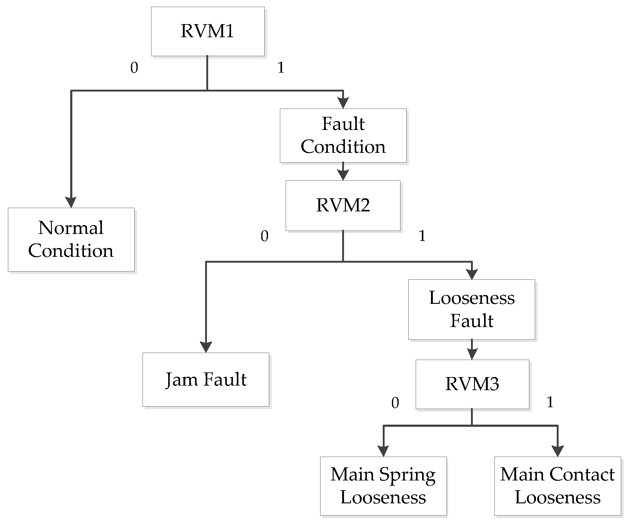
Figure 2.
Fault classification algorithm flow chart.

Figure 3.
Vibration test in the laboratory.

Figure 4.
Vibration signals under different conditions.

Figure 5.
Time–frequency diagram of the main contact looseness signal.
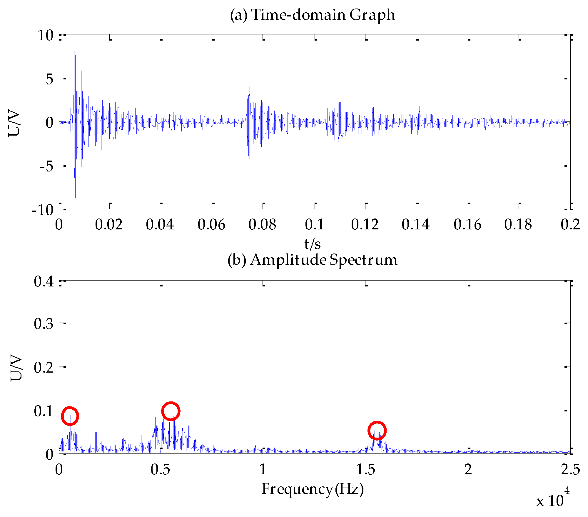
Figure 6.
Time–frequency diagram of IMF1–IMF3.

Figure 7.
Comparison between the reconstructed signal and the original signal.
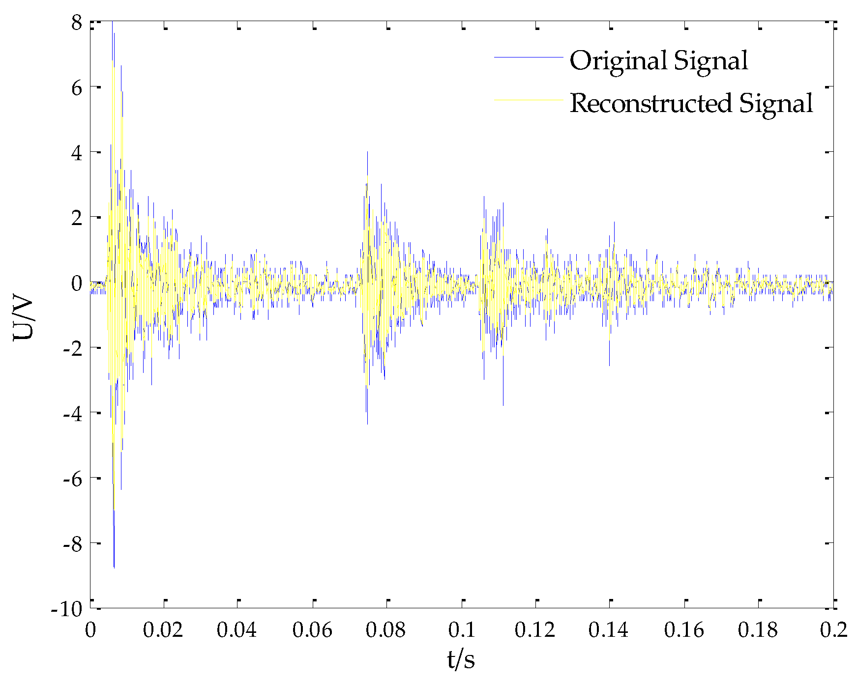
Figure 8.
Empirical mode decomposition (EMD) decomposition result.

Figure 9.
Ensemble empirical mode decomposition (EEMD) decomposition result.

Figure 10.
Distribution of weight divergence under different conditions.

Figure 11.
Fitness value curve. The selection of kernel parameters: δ1=1.181, δ2=0.123 and δ3=0.125.
Figure 11.
Fitness value curve. The selection of kernel parameters: δ1=1.181, δ2=0.123 and δ3=0.125.

Table 1.
Information regarding the experimental equipment.
| Equipment | Model | Origin |
|---|---|---|
| OLTC | SYJZZ | Shanghai, China |
| Piezoelectric Acceleration Sensor | YD70C | Qinhuangdao, Hebei Province, China |
| Charge Amplifier | DHF-10 | Qinhuangdao, Hebei Province, China |
| Oscilloscope | Tek 3034 | Shenzhen, Guangdong Province, China |
Table 2.
Decomposition results under different K values. The × means nothing in Table 2.
Table 2.
Decomposition results under different K values. The × means nothing in Table 2.
| Decomposition Level | Center Frequency/Hz | |||||
|---|---|---|---|---|---|---|
| 800 | 5000 | 5500 | 15,500 | 157,000 | 20,500 | |
| K = 2 | 0.09 | × | × | × | 0.052 | × |
| K = 3 | 0.09 | × | 0.1 | 0.052 | × | × |
| K = 4 | 0.09 | × | 0.1 | 0.052 | 0.037 | × |
| K = 5 | 0.09 | 0.09 | 0.07 | 0.052 | × | 0.008 |
Table 3.
Comparison of three algorithms.
| Algorithm | Parameter Settings | Operation Time | The Degree of Modal Aliasing |
|---|---|---|---|
| EMD | Default parameter | 0.771265 s | Graveness |
| EEMD | Nstd = 0.8; NE = 100 | 55.799760 s | Moderation |
| VMD | α = 2000; tau = 0.3; K = 3 | 2.162024 s | Absence |
Table 4.
The selections of training set and test set.
| Classifier | Condition of OLTC | Number of Training Set | Number of Test Set | Total |
|---|---|---|---|---|
| HS-RVM | Normal Condition | 10 | 10 | 20 |
| Main Contact Looseness | 10 | 10 | 20 | |
| Main Spring Looseness | 10 | 14 | 24 | |
| Jam Fault | 10 | 11 | 21 | |
| Total | 40 | 45 | 85 | |
Table 5.
Diagnostic results of harmony search optimization-relevance vector machine (HS-RVM).
| Data Set | Condition of OLTC | Diagnosis Results | Accuracy | |||
|---|---|---|---|---|---|---|
| Normal | Fault I | Fault II | Fault III | |||
| Training set | Normal | 10 | 0 | 0 | 0 | 92.5% |
| Fault I | 0 | 10 | 0 | 0 | ||
| Fault II | 0 | 1 | 8 | 1 | ||
| Fault III | 0 | 1 | 0 | 9 | ||
| Test set | Normal | 10 | 0 | 0 | 0 | 84.4% |
| Fault I | 0 | 9 | 0 | 2 | ||
| Fault II | 0 | 1 | 11 | 2 | ||
| Fault III | 0 | 1 | 1 | 8 | ||
Table 6.
The comparisons of test set diagnostic results.
| Classifier | Condition of OLTC | Diagnosis Results | Accuracy | |||
|---|---|---|---|---|---|---|
| Normal | Fault I | Fault II | Fault III | |||
| RVM | Normal | 10 | 0 | 0 | 0 | 68.9% |
| Fault I | 0 | 6 | 2 | 3 | ||
| Fault II | 0 | 1 | 10 | 3 | ||
| Fault III | 0 | 2 | 3 | 5 | ||
| SA-RVM | Normal | 10 | 0 | 0 | 0 | 77.8% |
| Fault I | 0 | 7 | 2 | 2 | ||
| Fault II | 0 | 1 | 12 | 1 | ||
| Fault III | 0 | 1 | 3 | 6 | ||
| HS-RVM | Normal | 10 | 0 | 0 | 0 | 84.4% |
| Fault I | 0 | 9 | 0 | 2 | ||
| Fault II | 0 | 1 | 11 | 2 | ||
| Fault III | 0 | 1 | 1 | 8 | ||
Table 7.
Test set diagnostic results of the EMD-SVM model.
| Model | Number of Training Sets | Number of Test Sets | Number of Errors | Accuracy |
|---|---|---|---|---|
| EMD-SVM | 40 | 45 | 17 | 62.2% |
| HS-RVM | 40 | 45 | 7 | 84.4% |
© 2017 by the authors. Licensee MDPI, Basel, Switzerland. This article is an open access article distributed under the terms and conditions of the Creative Commons Attribution (CC BY) license (http://creativecommons.org/licenses/by/4.0/).
Share and Cite
MDPI and ACS Style
Liu, J.; Wang, G.; Zhao, T.; Zhang, L. Fault Diagnosis of On-Load Tap-Changer Based on Variational Mode Decomposition and Relevance Vector Machine. Energies 2017, 10, 946. https://doi.org/10.3390/en10070946
AMA Style
Liu J, Wang G, Zhao T, Zhang L. Fault Diagnosis of On-Load Tap-Changer Based on Variational Mode Decomposition and Relevance Vector Machine. Energies. 2017; 10(7):946. https://doi.org/10.3390/en10070946
Chicago/Turabian StyleLiu, Jinxin, Guan Wang, Tong Zhao, and Li Zhang. 2017. "Fault Diagnosis of On-Load Tap-Changer Based on Variational Mode Decomposition and Relevance Vector Machine" Energies 10, no. 7: 946. https://doi.org/10.3390/en10070946
Note that from the first issue of 2016, this journal uses article numbers instead of page numbers. See further details here.