The results of the case study are organized as follows: first, the range extension provided by the electric bus is estimated. Next, the results are used to measure the amount of electrical energy that was collected per year from an OBPV system, compared to the annual consumption of electric energy by the bus. Third, the results are used to determine the impact of OBPV on battery aging, as compared to other methods of increasing battery life.
4.2. Photovoltaic Energy
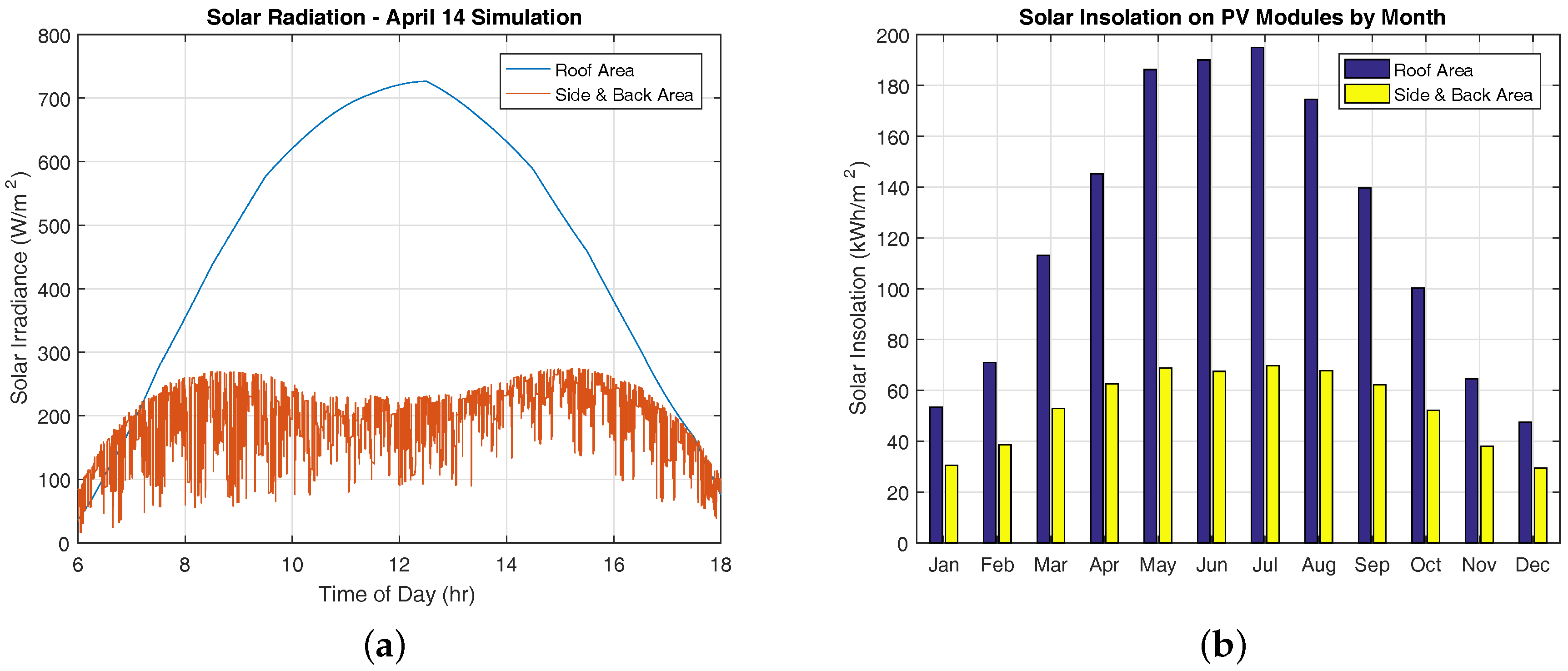
The intensities of solar radiation reaching the bus roof and bus sides were compared in terms of daily irradiance and monthly insolation.
Figure 17a shows the simulated radiation that reaches the bus on a fairly typical day. The side PV modules experienced more variation than the roof PV modules due to the changing bus orientation and also experienced a decrease in radiation during midday, when the sun was close to directly overhead. The side modules experienced less radiation in general because they could not always be exposed to direct radiation. However, near sunrise and sunset when the sun was low in the sky, sunlight reached the side modules at a more direct angle, such that the side modules experienced more radiation than the roof module.
Figure 17b shows the total solar insolation that reached the panels each month. In
Figure 17b, the total radiation on the side modules is found by taking a weighted average of the total radiation on the right, left, and back modules:
The insolation is found by integrating the radiation with respect to time. Because the bus traveled north, south, east, and west roughly equally, the insolations on the right, left, and back PV modules were approximately equal to each other regardless of time of year.
The sun is lower in the sky in winter months compared to summer months, so solar radiation approached the side modules at a more direct angle. In addition, greater cloud cover in the winter months meant that the diffuse radiation made up a larger portion of the total radiation. This resulted in less discrepancy between the Rooftop PV modules and side PV modules during winter months compared to summer months. The total yearly solar insolation was 1480 kWh/m on the roof module and 640 kWh/m on the side modules.
Assuming the PV modules could continue to collect energy and charge the battery while the bus was not in operation, the roof-mounted panels collected a total of 4560 kWh of electrical energy over one year, while the side-mounted panels collected a total of 4321 kWh of energy.
Figure 18 shows the electrical energy from PV modules by month. The electrical energy is found by integrating Equation (
55), where the solar radiation and ambient temperature for each day of the year are obtained from the NREL’s TMY data [
55]. Because the side modules covered a larger area than the rooftop modules, they produced a comparable amount of electrical energy to the rooftop modules despite their lower annual insolation.
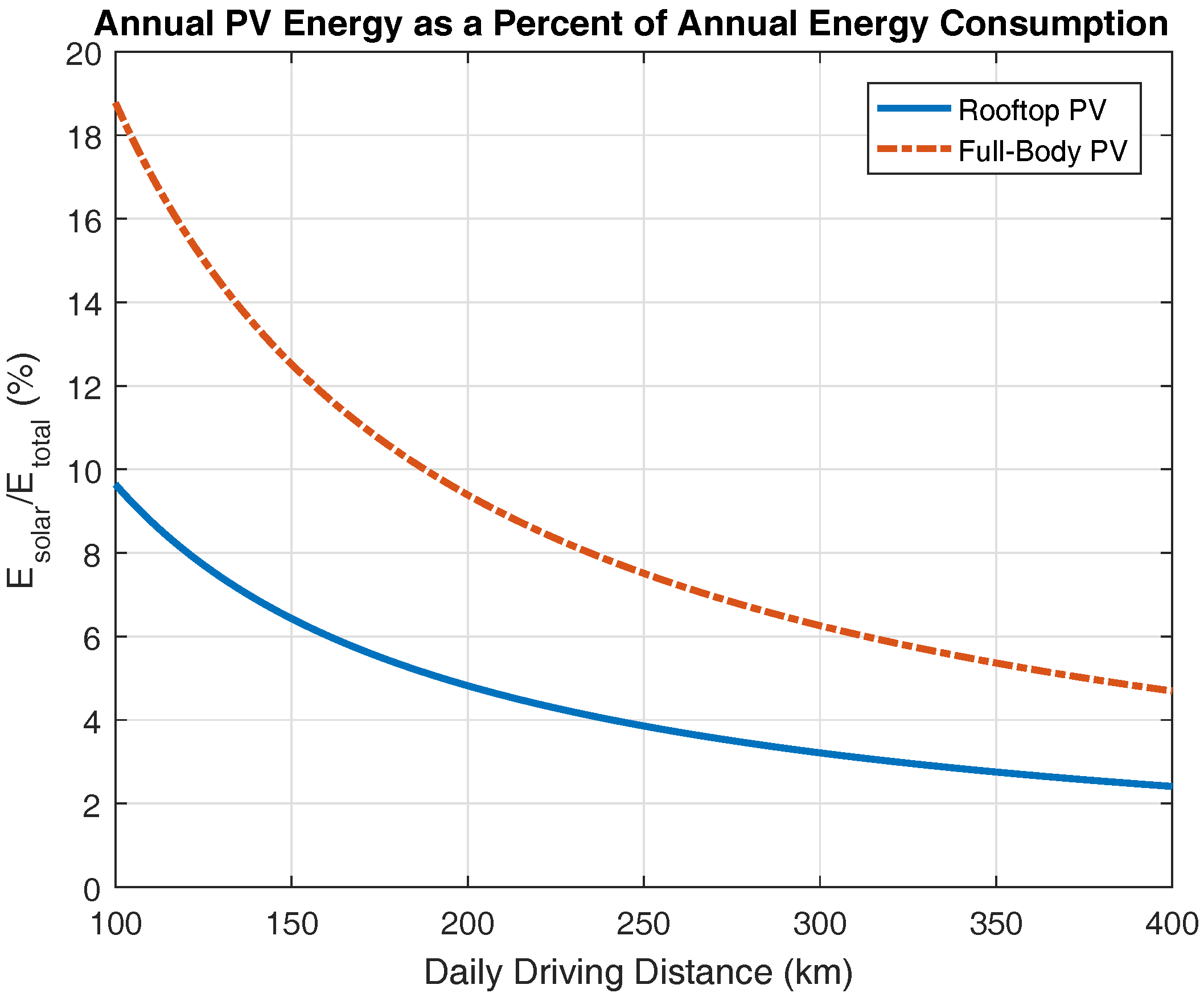
Using the fuel economy results presented earlier, one can estimate the portion of the annual electrical energy consumption of the bus that the PV modules can provide for various daily route lengths. For instance, if a bus is driven 150 km each day, Rooftop PV modules could provide up to 6.4% of the electrical energy, while modules on the roof and sides could together provide up to 12.5%. The relation between this percentage and the average daily driving distance is illustrated in
Figure 19.
An interesting finding was that although the side-mounted PV panels provided less power in summer months, they provided as much or more power than the Rooftop PV modules during the winter months. This was because, in winter months, the earth is tilted away from the sun, resulting in the radiation having a more direct path to the side modules than in summer months. Although the side PV modules were less efficient on a per-area basis, they reduced the variability in daily energy collected between summer and winter months.
The payback time can be computed for the top and side PV modules using the commercial off-peak cost of energy in Davis,
$0.23 per kWh [
57]. Using the industrial average price per watt of solar panels, it is estimated that the rooftop module would cost
$6247, while the side modules would cost
$13,139 [
53]. Then, the rooftop panels are expected have a payback time of six years, while the side panels are expected to have a payback time of 13 years and three months. These payback times are longer than the amount estimated in [
4,
13] due to the lower price of electric energy compared to diesel fuel. For payback times of this length, it is questionable whether a manufacturer would want to go ahead with PV integration. However, these payback times do not account for any incentives that local government might offer for solar installation, nor do they account for the value added from extending the battery cycle life, which will be discussed in
Section 4.3.
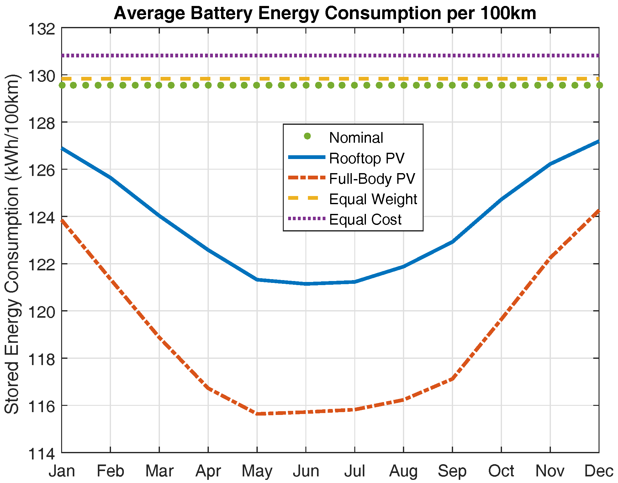
4.3. Battery Aging
Repeated simulations were carried out for each configuration to find the battery cycle life associated with each configuration and route duration. In this section, one “cycle” refers to one day of driving. The nominal, equal weight, and equal cost configurations did not have any weather-dependent parameters, so the only variation from one simulation to the next was the maximum battery capacity. On the other hand, the Rooftop PV and Full-Body PV configurations had weather conditions that changed daily in addition to the changing maximum battery capacity. These experiments were carried out using chronological TMY data.
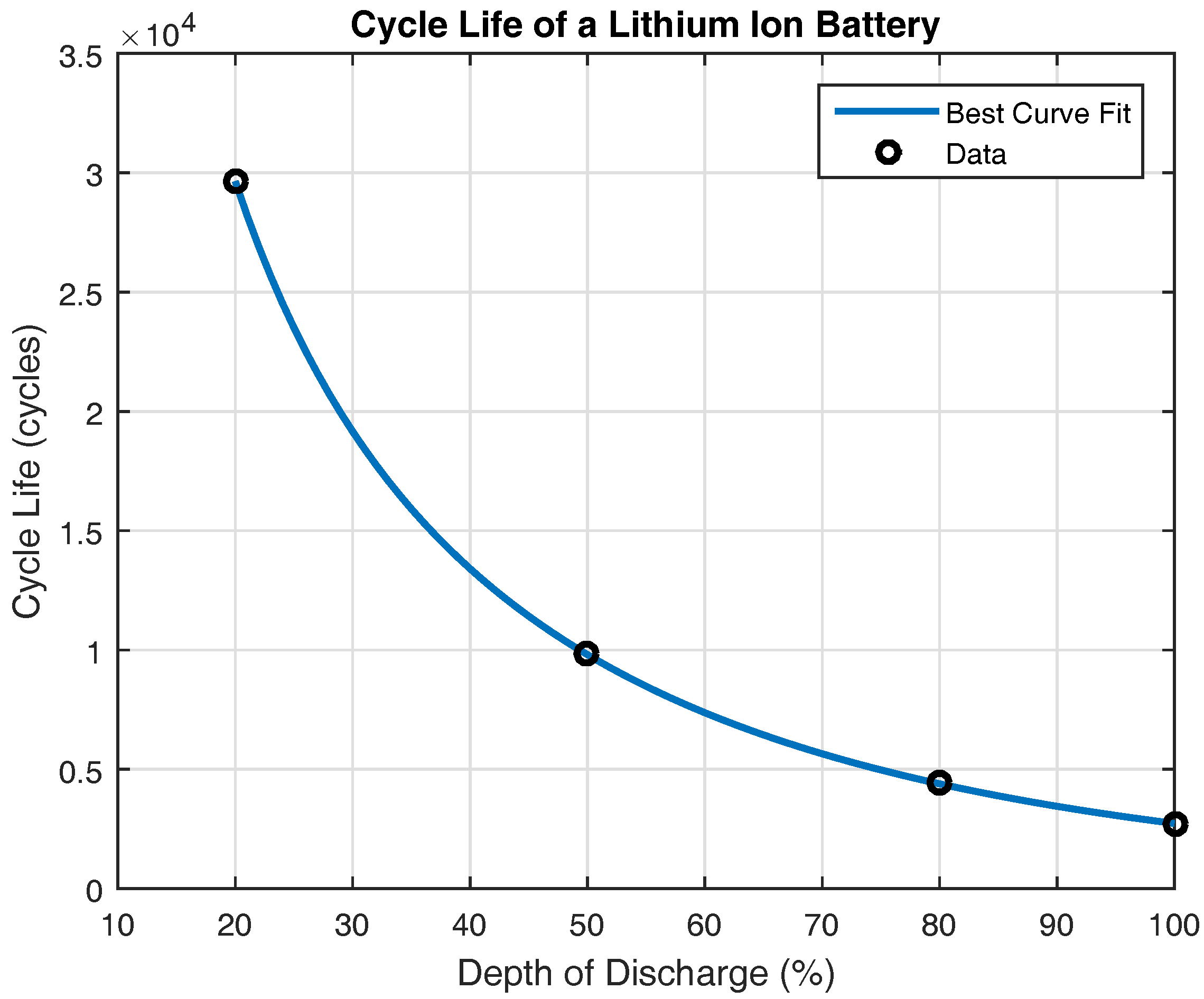
Before proceeding to the battery aging results, some of the aging modeling assumptions are verified. The battery aging model assumed that the charge and discharge rates, as well as the difference in charge and discharge rates between configurations, would be small enough that the aging model would only need to consider the depth-of-discharge per cycle. It was observed from the results that the average absolute
C-rate for the nominal bus was 0.169 C, while it was 0.166 C for the Rooftop PV configuration and 0.165 C for the Full-Body configuration. These rates are low and near 0.5 C, the
C-rate of the test data in [
34]. Additionally, the maximum discharging
C-rates were 0.777 C, 0.768 C, and 0.764 C, respectively, while the maximum charging
C-rates were 0.968 C, 0.977 C, and 0.992 C. Because the
C-rates were low and near the
C-rate of the empirical cycle life data, and because the differences in
C-rate between the configurations were minimal, the assumption that charge and discharge rates could be neglected from the aging model was considered valid.
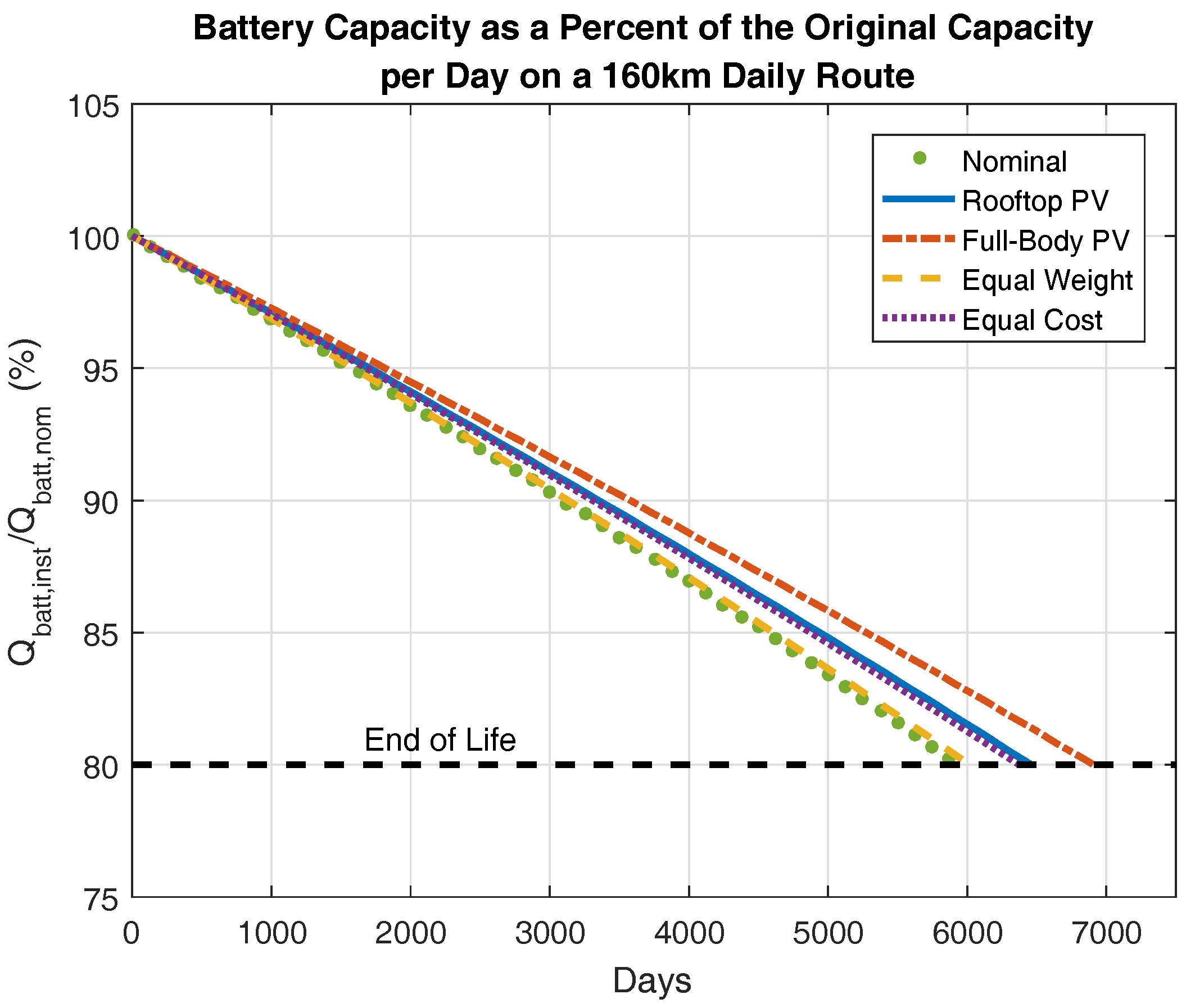
Figure 20 shows the aging of the five different configurations for a 160 km daily bus route. The battery for the nominal configuration aged the fastest, reaching its end-of-life after approximately 6000 charge-and-discharge cycles—or rather, approximately 6000 days of driving. The Full-Body PV configuration aged the slowest, followed by Rooftop PV and then the two extra-battery configuration. For each configuration, as the maximum storage capacity of the battery decreased with each day of driving, it was discharged to greater depths, which, in turn, caused each cycle to do more damage.
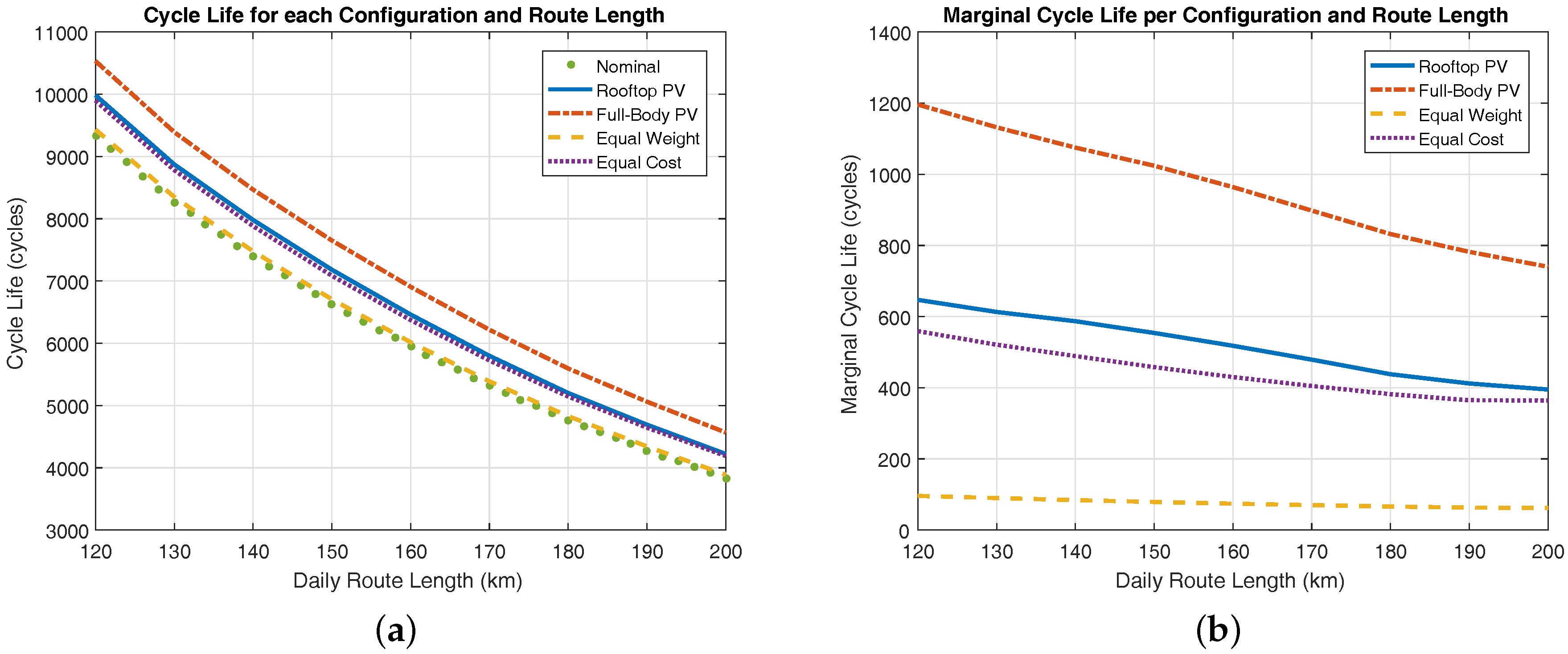
Figure 21a shows the cycle life for each configuration as it varies with route length, while
Figure 21b shows the increase in cycle life of each configuration over the nominal configuration at each route length. Although the marginal cycle life for each configuration increased with decreasing route length, the percentage increase in cycle life was greater for longer routes. The Full-Body PV configuration increased the battery cycle life the most, followed by the Rooftop PV, then the Equal Cost, and finally the Equal Weight configuration.
Increased cycle life on its own is not necessarily a good metric for each configuration’s performance. Each configuration would have different drawbacks, such as added mass, size, or installation cost. The additional benefits of each configuration should therefore be compared to the additional penalty incurred by implementing that configuration.
This paper first considers the marginal mass of each configuration. If the added PV modules or battery cells add too much weight, it might require the manufacturer to redesign other components of the bus or reduce the allowable number of passengers. The marginal mass of each configuration is summarized in
Table 5.
Additionally, each configuration was looked at in terms of the effort required to implement that configuration. “Effort to implement” might include cost to install each configuration, ongoing maintenance costs, or additional hardware, such as a larger battery management system. This paper considers the estimated marginal cost of the configuration, in terms of the industrial average price per watt of PV panels and price per kilowatt-hour of lithium-ion batteries, to be a reasonable proxy variable for “effort to implement”. The price per kilowatt-hour for lithium-ion batteries is provided by [
52], while the price per watt of PV systems is from [
53]. The marginal cost of each configuration is summarized in
Table 5.
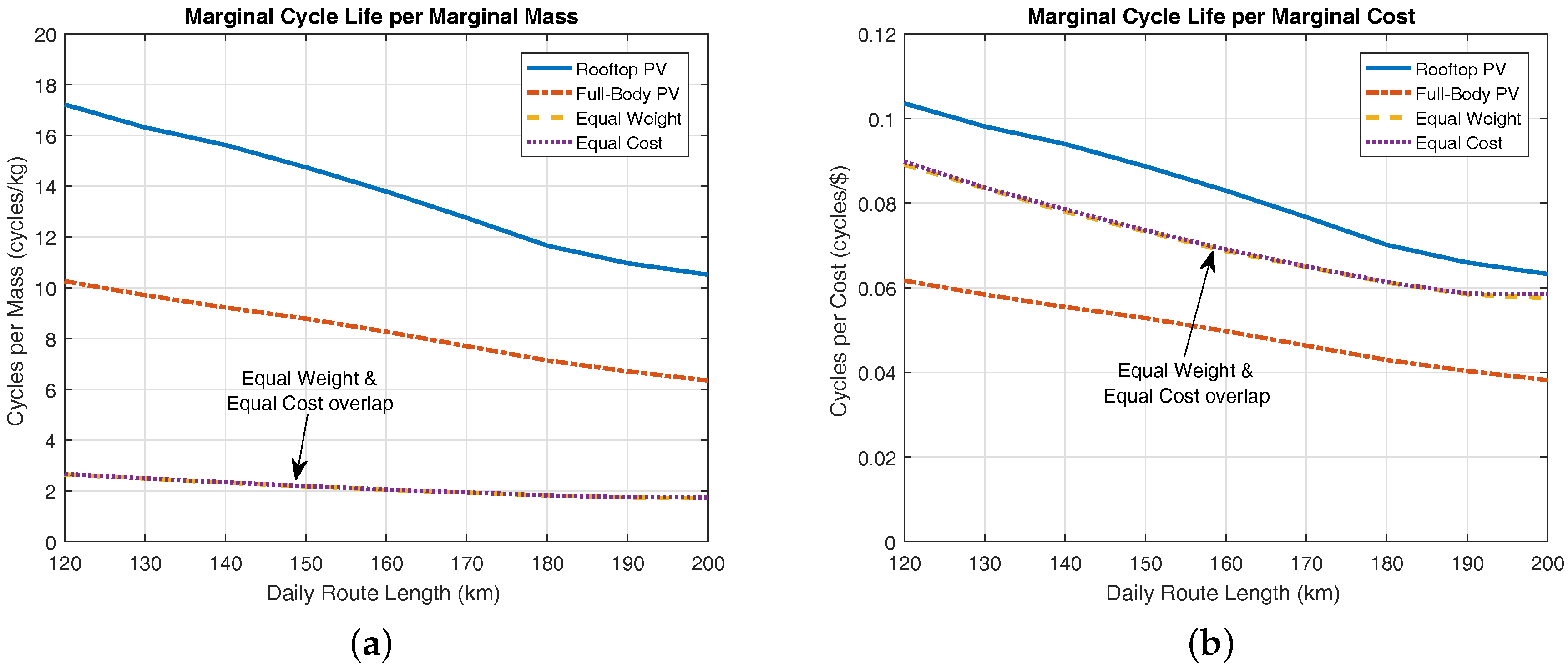
Figure 22a shows the marginal cycle life per marginal mass for each configuration and route length. Although the Full-Body PV configuration yielded the most additional cycles, the Rooftop PV configuration was a more effective use of mass. In general, adding PV modules to the bus was a more effective use of weight than increasing battery size.
Figure 22b shows the marginal cycle life per marginal cost for each configuration and route length. Due to the low amount of radiation that the side modules experienced, the Full-Body PV configuration was the most inefficient use of funds. Although the Equal Weight configuration added the fewest cycles, its marginal cycle life was achieved at very little expense. Both added-battery configurations outperformed the Full-Body PV configuration, but the Rooftop PV configuration was clearly the most cost-effective.
These relationships are visualized with the radar charts shown in
Figure 23a–d. It should be noted that these plots use the inverse of marginal cost and marginal mass. This is done so that a large value corresponds to a desirable trait: large “per cost” indicates an inexpensive option, while large “per mass” indicates a low-weight option. The axes of these plots are scaled so that the largest marginal cycle life, inverse marginal cost, and inverse marginal mass across the four cases are all the same distance from the origin. Although the Rooftop PV and Equal Cost configurations had the same initial cost, the Rooftop PV configuration provided moderately longer cycle life and was a much more effective use of weight. The Full-Body PV provided the largest extension to battery life, but was neither as cost or weight effective as PV modules on the bus roof only. The Equal Weight configuration was both low-cost and low-weight, but provided little in the way of additional battery lifespan. Overall, the Rooftop PV configuration offered the best balance of extending battery cycle life while keeping weight and cost low.
Alternatively, one could define a non-dimensional cost or reward function to compare the four configurations with a single metric. For example, Equation (
57) is a reward function that increases with larger cycle life improvements and decreases with larger costs at rates defined by the weighting parameters
,
, and
, where
is the average marginal cycle life,
is the marginal mass, and
is the marginal cost:
One could select
,
, and
, which normalizes the three variables so that, among the four configurations, the reward due to the maximum mean marginal cycle life is equal to the combined penalty of the maximum marginal mass and maximum marginal cost. The resulting reward/penalty of each configuration for this function and weighting are shown in
Figure 24. Once again, the Rooftop PV configuration strikes the best balance between added cycle life and added cost and weight. The higher weight lower marginal cycle life of the larger-battery configurations result in a net penalty rather than reward, indicating that OBPV is a better choice to extend battery lifespan. Of course, these results are heavily dependent on the choice of reward function.
A final metric for assessing the value of each configuration is the return on investment from an increase in cycle life. The nominal configuration was estimated to cost
$118,580. Then, the cost per cycle of the nominal configuration can be estimated by dividing the estimated cost by the nominal configuration cycle life
:
The value of the cycles added by each configuration can then be found by multiplying the nominal cost per cycle by the marginal cycle life
of a given configuration:
The net profit or loss is found by subtracting the marginal cost
of a given configuration:
Return on investment (ROI) is then found by normalizing by the marginal cost of that same configuration and expressing the result as a percent:
Here, indicates the break-even point, while indicates that the value of the added cycle life is twice the estimated cost of the configuration.
The ROI for each configuration and daily driving distance are shown in
Figure 25. For all configurations, the ROI is greater with longer daily driving distances—or, rather, for routes where the battery is discharged to a greater depth. The Rooftop PV configuration is seen to provide a positive ROI for all route lengths, while the Full-Body PV configuration is a net loss until the daily driving distance reaches 160 km. The added-battery configurations are beneficial, but not to the extent of the Rooftop PV configuration.


