
A Piecewise Bound Constrained Optimization for Harmonic Responsibilities Assessment under Utility Harmonic Impedance Changes


1
School of Electrical Engineering, Southwest Jiaotong University, Chengdu 610031, China
2
Guizhou Key Laboratory of Electric Power Big Data, Guizhou Institute of Technology, Guiyang 550003, China
3
State Key Laboratory of Security Control and Simulation of Power Systems and Large Scale Generation Equipment, Department of Electrical Engineering, Tsinghua University, Beijing 100084, China
*
Author to whom correspondence should be addressed.
Energies 2017, 10(7), 936; https://doi.org/10.3390/en10070936
Submission received: 22 April 2017
/
Revised: 25 June 2017
/
Accepted: 1 July 2017
/
Published: 6 July 2017
(This article belongs to the Special Issue Distribution Power Systems and Power Quality)
Abstract
:Considering the effect of the utility harmonic impedance variations on harmonic responsibility, a method based on piecewise bound constrained optimization is proposed in this paper to evaluate the load harmonic responsibilities. The wavelet packet transform is employed to determine the change times of the utility harmonic impedances. The harmonic monitoring data is divided into several segments where the utility harmonic impedances are considered as constants. Then, the problem of harmonic responsibility assessment under utility harmonic impedance changes are settled by the piecewise bound constrained optimization model. Furthermore, the interior point, the sequential quadratic programming and the active set algorithm are respectively adopted to calculate all the instantaneous harmonic responsibilities of harmonic loads. Finally, the weighted summation is used to calculate the total harmonic responsibility. To demonstrate the validity, simulation tests are carried out on an experimental circuit and the IEEE 13-bus distribution system.
1. Introduction
With the development of smart grids, increasing numbers of power electronic devices have been connected to distribution networks, which inject a large amount of harmonics [1,2,3,4,5]. Various electrical power equipment and electronic products have a strong sensitivity to the harmonics in the distribution network, making harmonic elimination of great importance [6]. To address the problem of harmonic pollution, appropriate punishment scheme should be executed according to the harmonic limits recommended by the IEEE or IEC standards. To ensure its implementation, it is necessary to quantitatively evaluate the harmonic responsibility of the major harmonic loads at the point of common coupling (PCC) in distribution networks [7,8,9].
In traditional methods, the key of harmonic responsibility evaluation is to determine the utility harmonic impedance. These works can be mainly classified as fluctuation quantity methods [10,11], linear regression methods [12,13,14] and independent component analysis (ICA) [15,16] methods. Fluctuation quantity methods rely on the fluctuation quantity proportion of harmonic voltage to current for calculating the harmonic impedance. The various regression analysis methods, such as the complex linear least squares [12], non-parametric regression [13] and multiple linear regression [14] methods, formulate an equation and solve the regression coefficient so as to get the utility harmonic impedance. The complex ICA [15] and FastICA [16] are usually used to estimate the utility harmonic impedance when the utility harmonic variations are neglected. Meanwhile, most of the above methods are based upon the supposition that the utility harmonic are invariant. In a real power grid, the utility harmonic voltage fluctuates due to the load fluctuation. The utility harmonic voltage has a certain influence on the amplitude as well as angle of the harmonic current which affects the harmonic voltage [17,18]. Under certain condition, the harmonic voltage and current all fluctuate simultaneously. The methods above cannot reflect the variation of harmonic voltage and current while the influence of utility harmonic voltage fluctuation is considered in [19,20,21]. In the previous study of the authors, an adaptive assessment approach [19] for harmonic responsibility under utility harmonic voltage variation was proposed. It has been proved that the utility harmonic voltage can be segmented by hierarchical K-means clustering under the condition of the same utility harmonic impedance. Then, regression methods can be effectively used to calculate the harmonic responsibilities. In the study of utility harmonic voltage fluctuation, the utility harmonic impedance is supposed to be invariant, but the switching of the equipment [22], changes in the reactive power compensation, the state of the distributed generators and the adjustment of the interruptible loads [23] can all result in variations in utility harmonic impedance. Under such an unrealistic assumption, a series of errors may be introduced in the assessment results. Therefore, it is of great significance to evaluate the harmonic responsibility in the presence of utility harmonic impedance changes.
Based on the analysis above, and considering the utility harmonic impedance changes, this paper firstly adopts the wavelet packet transform to detect the change points of the utility harmonic impedance. Then, the harmonic measurement data are segmented. Besides, in order to more accurately evaluate harmonic responsibility, the piecewise bound constrained optimization model and nonlinear optimization method are used to calculate the responsibility of each segment. Finally, the total harmonic responsibility of each harmonic load is obtained based on the data segment length. Section 2 describes the basic principles and conventional method of harmonic responsibility assessment. In Section 3, determination method of the change times of utility harmonic impedance is formulated. Section 4 introduces the piecewise bound constrained optimization method for harmonic responsibility assessment. The process of the novel method for harmonic responsibility assessment, numerical experiments and conclusion are provided in Section 5, Section 6 and Section 7, respectively.
2. Basic Principle and Conventional Method of Harmonic Responsibility Assessment
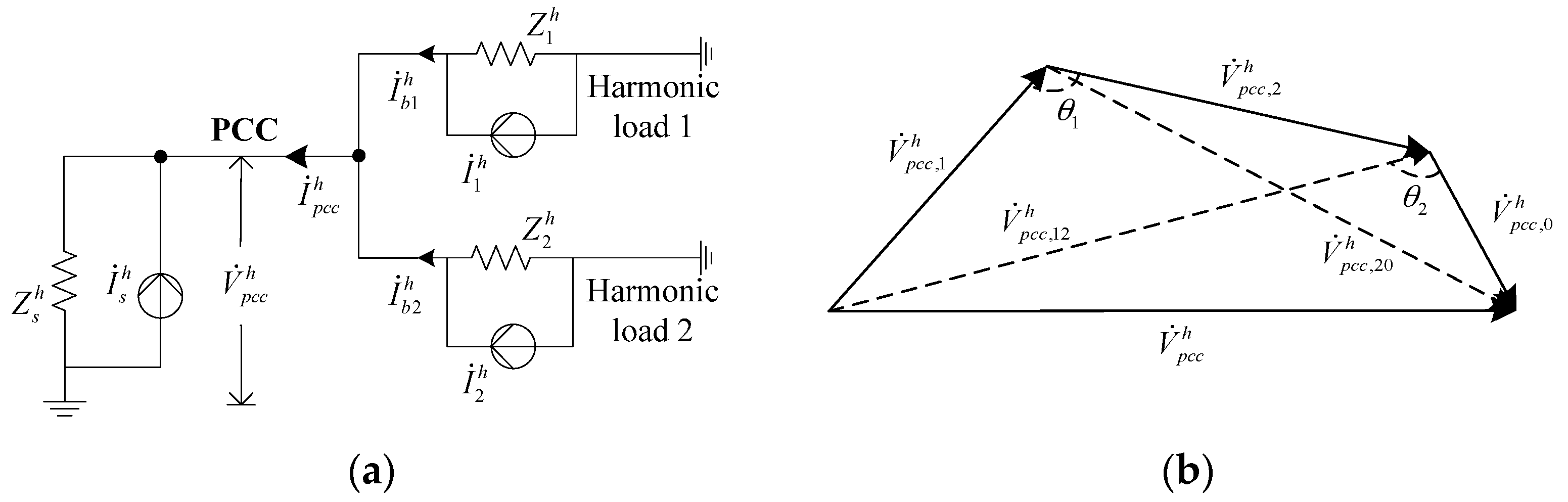
The Norton equivalent circuits can be applied for harmonic modelling of utility and loads [19,24]. Figure 1a shows a typical distribution system with two major harmonic loads, where h stands for the harmonic order; and are the equivalent harmonic impedance and injected current at the utility side, respectively, while and are the equivalent harmonic impedance and injected current of each nonlinear load; is the branch harmonic current; and are the h-th harmonic voltage and current at the PCC, respectively.
According to the superposition principle, the h-th harmonic voltage at the PCC is:
where dots represent the phasors of the voltages or currents, and denote the harmonic voltage at harmonic load 1 and 2 at the PCC, respectively; and are the equivalent harmonic impedance but harmonic load 1 or 2, respectively; is the harmonic voltage from the utility at the PCC, also known as the utility harmonic voltage. The phasor diagram of the h-th harmonic voltages is shown in Figure 1b.
The harmonic responsibility of harmonic load i (i = 1, 2) at the PCC can be calculated as:
where is the phase angle between and .
Linear regression is a common assessment method for harmonic responsibilities [12,13], which is based on monitoring the harmonic voltage and current at the PCC.
The normalized h-th harmonic voltage and current at the PCC are related by:
Figure 1 indicates the harmonic voltage at the PCC is:
Let , , and then can be expressed as:
It can be seen from Equations (3)–(5) that in the application of linear regression methods, the harmonic data should meet that the change of the utility harmonic voltage cannot influence the change of the harmonic current. Furthermore, if either the harmonic voltage, current or impedance changes, the accuracy of the regression analysis will be affected. Therefore, the variations of utility harmonics are the main error sources when the regression methods are employed.
3. Determination of the Change Time of Utility Harmonic Impedance Using Wavelet Packet Transform
In the distribution system, the changes of the operation mode, load or reactive compensation can all lead to changes of the utility harmonic impedance. To accurately calculate the harmonic responsibility, harmonic monitoring data must be properly segmented according to the identified utility harmonic impedance. In this article, the roughly estimates of utility harmonic impedance are used to segment the data.
Due to the complexity of the actual distribution system and the existence of transient processes, the actual utility harmonic impedance changes in a gradual manner. Therefore, it is necessary to choose an effective method to adaptively detect the change. In view of the good performance of wavelet package transform in signal singularity detection, this paper employs the wavelet package transform to detect the change points of the utility harmonic impedance.
In wavelet packet transform, the input signal can be decomposed into low frequency and high frequency components level by level to represent the approximations and details of signal respectively [25]. Figure 2 shows a wavelet packet transform tree with three decomposition levels. The wavelet packet coefficients at each level can be obtained by:
where and represent a low-pass filter and a high-pass filter, respectively; is the sampling point; is the displacement factor; represents the component at the level j − 1, and represent the low frequency and high frequency components at the level j, respectively.
The main idea of identifying the variation of utility harmonic impedance using wavelet packet transform is described in the following paragraphs. Since the boundary of the utility harmonic impedance change is not obvious, this paper transforms the identification of change point into the identification of change time window by adding windows, in order to reduce the identification error. The window length is denoted by L. According to Equation (3), if the values of the load harmonic impedances and injected harmonic currents can be considered as constants, the slope of the fitting curve is then a rough estimate of the utility harmonic impedance, and the slopes are approximately equal in this period. If mutation exists in the utility harmonic impedance, the slope of the fitting curve will change sharply compared with the adjacent window.
With regard to small samples, the window length L = 3 can be used to carry out the regression analysis. In the harmonic responsibility assessment, the data points in the time window, which correspond to the mutational utility harmonic impedance, are deleted. The sampling data points in the segments on both sides of the deleted time window can be considered as the data points under the same utility harmonic impedance.
For large samples, a long window length, such as L = 30, should be used to carry out the regression analysis, and the utility harmonic impedance change time can be directly determined through the wavelet packet decomposition curve.
Since high frequency components can reflect the mutational point of the signal, the high frequency band , and and obtained by wavelet packet transform are used. Set the threshold value , where M is the sampling number, is the standard deviation of the high frequency band signal, , represents the wavelet packet coefficients of a high frequency band and its mean is . The value below the threshold T is considered to be noise, and the value above T that is the mutation of the signal. Set A, B, and C as the sampling point sets of the change time window in the high frequency band , and respectively. According to the importance of the three high frequency components, in this article, the change time window of the utility harmonic impedance determined by:
4. The Piecewise Bound Constrained Optimization Model of Harmonic Responsibility Assessment and Its Solution Algorithms
In order to accurately calculate the single sampling point harmonic responsibility and the total harmonic responsibility of harmonic loads, upon the segmentation of the harmonic monitoring data, the harmonic responsibility is then assessed by the piecewise bound constrained optimization in this paper. According to the law of cosines [26], for the triangle XYZ:
where represents the angle contained between sides of lengths x and y and opposite the side of length z.
For simplicity, let , , , , , and . In order to estimate the independent variables , the absolute value of square error can be used as the objective function. The bound constrained optimization model is established as:
where ; T is the number of sample points; is the calculated value of harmonic voltage, , and are the measured values of harmonic voltage and currents respectively.
Once the estimated is obtained, according to Equation (2), the harmonic responsibility from two major harmonic loads, for each sampling point at ti can be calculated as:
Assuming that the monitoring data is divided into N segments and each segment corresponds to different utility harmonic impedance, the harmonic responsibility at each segment can be determined by:
where is the number of data points in the segment .
Total harmonic responsibility can be calculated by:
where is the harmonic responsibility of segment j; is the weight of each segment.
Numerous methods have been developed to figure out the bound constrained optimization problem. In this article, the interior-point (IP), the sequential quadratic programming (SQP) and the active set (AS) algorithm, which are all regarded as effective tools for solving nonlinear optimization problems, are selected.
A typical constrained programming problem can be expressed as:
The interior-point [27] for constrained optimization is mainly used to solve a variety of approximate optimization problem. For each the approximate model can be expressed as:
where denotes the slack variable. As decreases to 0, the minimum of approaches to the minimum of f.
The SQP [28] is a kind of approximate Newton’s method for solving constrained optimization problems. In each major iteration, the quasi-Newton updating method is firstly used to approach the Hessian of the Lagrangian function. The result is then employed to solve the QP (17) sub-problem:
where and .
For the constrained optimization problem, the following equation can be derived by Newton’s method:
where is the multiplier; denotes the Lagrangian expression for (17); and represents the Hessian of the Lagrangian.
The active set [29] solves the constrained optimization problem by determining the constraints that impact the results. Equation (15) can be rewritten as:
where A(γ) is a n-dimensional vector containing the evaluated values γ.
In the AS algorithm, the solutions of the Karush-Kuhn-Tucker (KKT) equations can be used to calculate the Lagrange multipliers (Li, i = 1, 2, ..., n). For Equation (19), the KKT equations can be expressed as:
Equation (20) demonstrates a cancelling of the gradients between the objective function and the active constraints at the solution point. Since the cancelling operation only involves active constraints, the Lagrange multipliers are therefore equal to 0.
5. The Proposed Harmonic Responsibility Assessment Approach
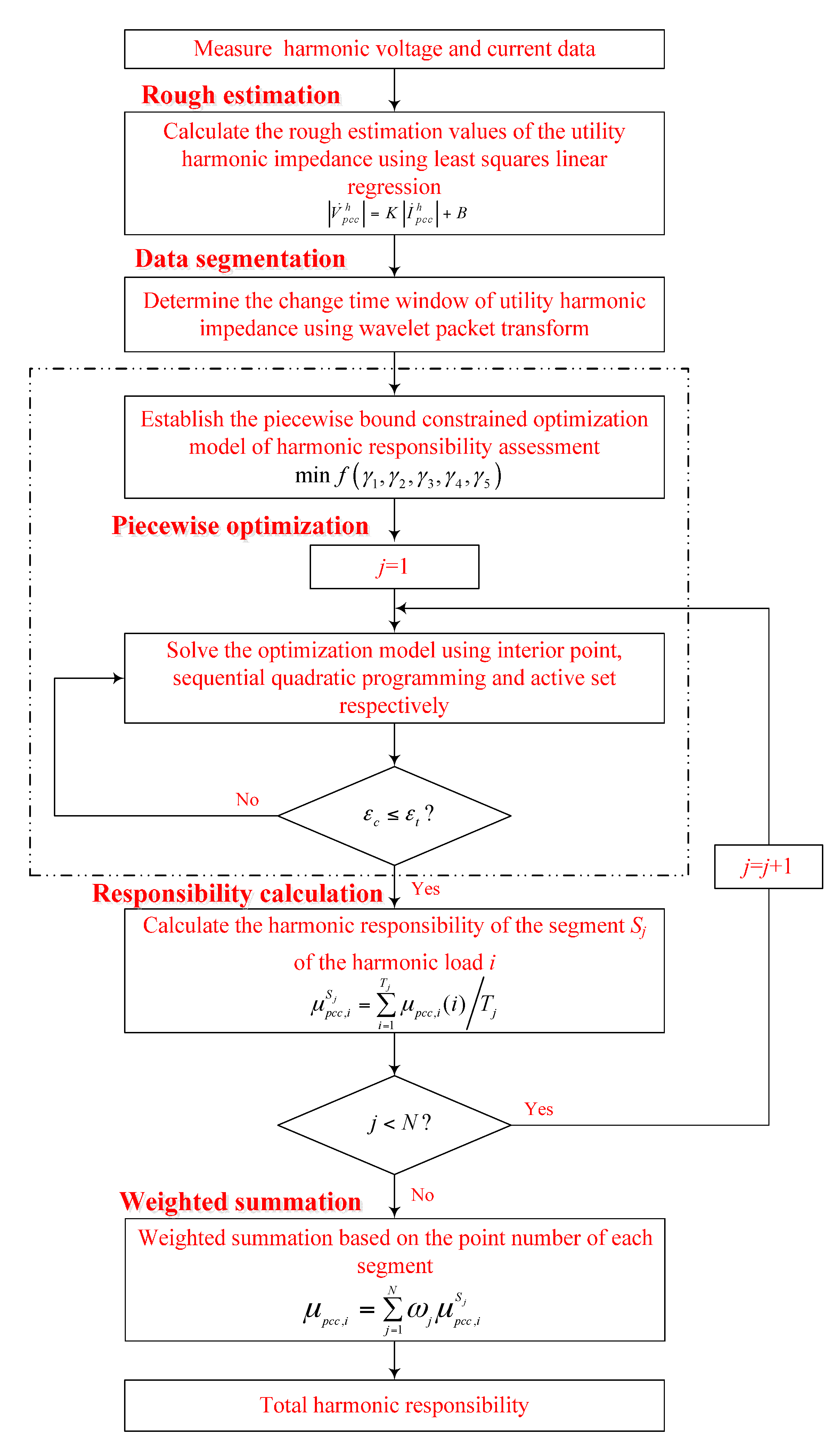
The working process of the proposed method for harmonic responsibility assessment is illustrated in Figure 3, where and represent the calculation error and the termination tolerance. Firstly, the utility harmonic impedance is roughly calculated by least squares linear regression. Second, the change time windows of the utility harmonic impedance are identified by the wavelet packet transform. Then, the harmonic responsibility of each segment is evaluated by the piecewise bound constrained optimization method. Finally, the total responsibilities of harmonic loads can be obtained by the weighted summation, based on the point numbers of segments.
6. Numerical Experiments
For the distribution system with two major harmonic loads as shown in Figure 1a, a Norton equivalent circuit model is established in MATLAB [30]. Taking the fifth harmonic as example, Table 1 presents the setting of parameter values. The harmonic impedance is modelled as the resistance R and reactance L in series. The system parameters and the injected harmonic currents are set and modified on the basis of [24]. In order to simulate practical engineering data, stochastic fluctuations are added to the harmonic data. For harmonic load 1 and 2, the means of the injected harmonic current data are 2.0788 + j0.1356 (A) and 3.8849 − j0.8549 (A) respectively, while the variances are 0.0018 and 0.0061 respectively. For the utility side, the mean of the injected utility harmonic current is 1.0243 − j0.3233 (A). The variances of all the harmonic impedances are 0.001. A total of 1440 harmonic sampling points of harmonic voltage and current data are generated. The change time of utility harmonic impedance are set as 501 and 1001.
For all the measured harmonic data, the least squares are used to carry out linear regression when the value of significance level is 0.05, and the regression coefficient is:
where are the estimated values of in Equation (5), that is, .
The 95% confidence intervals for the coefficient estimations are:
The R2 statistic, the F statistic and its p value can be calculated as R2 = 4.44781 × 10⁻⁴, F = 0.3219 and p = 0.7248, respectively. From the above results, the R2 statistic and the F statistic are insignificant, and p > 0.05. It is indicated that the regression should be rejected, and the harmonic responsibilities cannot be accurately calculated by the linear regression method under the changes of utility harmonic impedance. Thus, identifying the change times of the utility harmonic impedances is considered in this paper. It is solved by the wavelet packet decomposition method.
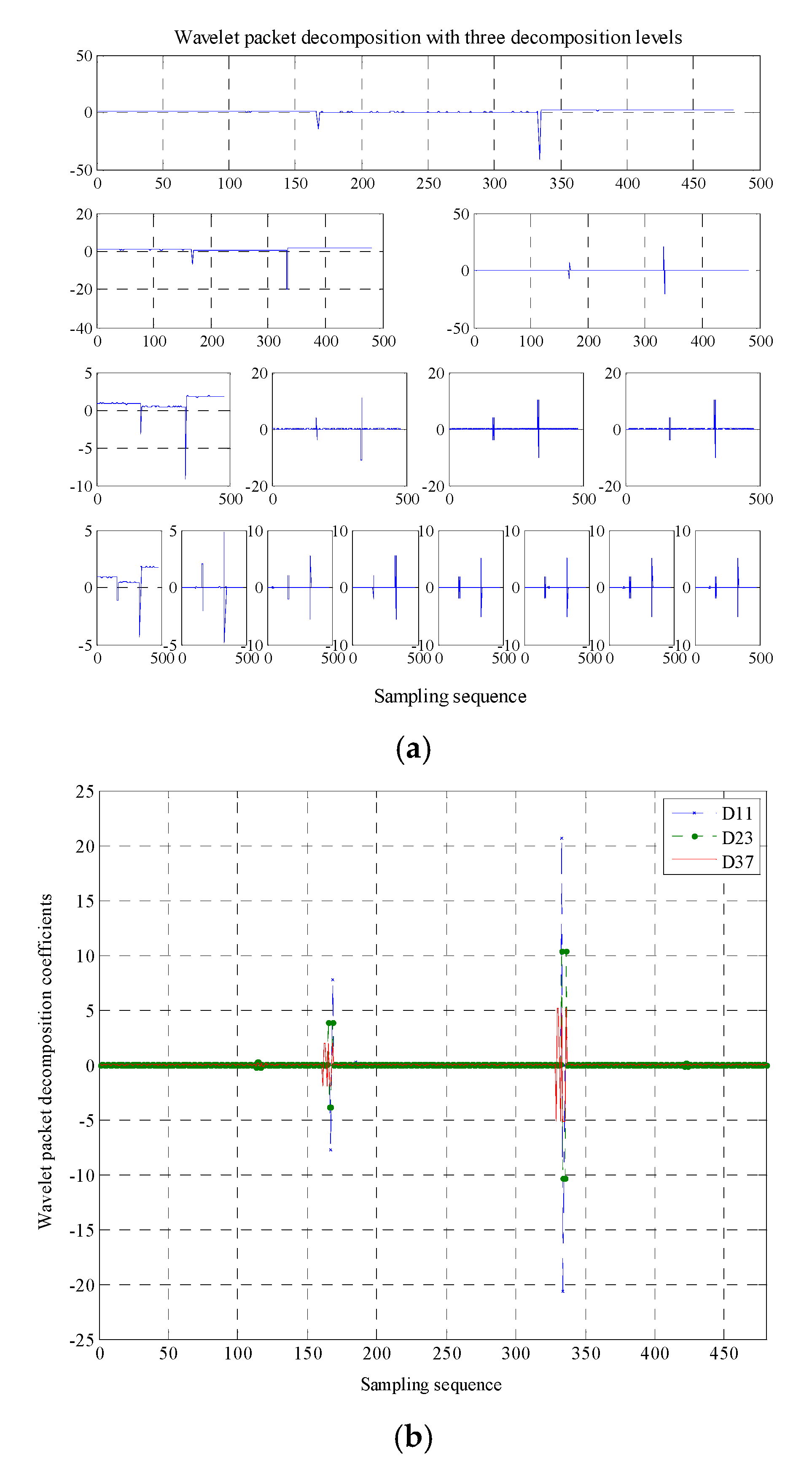
The wavelet packet decomposition results of the rough estimation of utility harmonic impedance using the Haar wavelet bases function are shown in Figure 4a,b. In order to select the appropriate wavelet basis, the Haar wavelet ‘haar (db1)’, Daubechies wavelet ‘db4’, Symlet wavelets ‘sym1’ and ‘sym4’, Coiflet wavelet ‘coif4’, and Demy wavelet ‘dmey’ [31] are used respectively to perform analysis and compared in this paper. The identification results of the change time window of utility harmonic impedance under different wavelet bases are shown in Table 2. As the sampling window length is 3, the sampling points of utility harmonic impedance changes set preciously (501 and 1001) are all included in the change time windows determined by wavelet packet transform. It can be seen from Table 2, the various wavelet basis functions can all deliver good performances in identifying the change time window, especially for haar (db1) and sym1 wavelet.
According to the change time window of the utility harmonic impedance [167, 168, 333, 334, 335, 336] determined by wavelet packet transform with haar wavelet, the sampling points (499–504) and (997–1008) are deleted. Then, the harmonic data are divided into three segments, that is (1–498), (505–996) and (1009–1440).
On the basis of data segmentation, the piecewise bound constrained optimization methods with three algorithms are used respectively to assess the harmonic responsibility. To accelerate convergence, the least square is adopted to solve the regression coefficients, which are taken as the initial values of the load harmonic impedances and . Then, the boundary constraints of the load harmonic impedances are set as and . The initial values for the cosine of phase angle value are set to be 0. Since in general, the initial values and the boundary constraint of are set to be and , which means the initial value of the independent variable is , and the boundary constraint values are and . The implementation of IP, SQP and AS are based on the ‘fmincon’ function in MATLAB. In order to ensure the fairness of algorithm comparison, the parameter settings of the three algorithms in Matlab are modified as follows. The maximum number of iterations is 1000, the maximum number of function evaluations is 5000, the termination tolerance is 1 × 10⁻¹⁰, and the values of other parameters are the default values of the ‘fmincon’ function [30].
For each segment, the theoretical harmonic responsibilities and calculated values obtained by the three algorithms, as well as the means and variances of the relative error between the calculated value and the theoretical value are presented in Table 3.
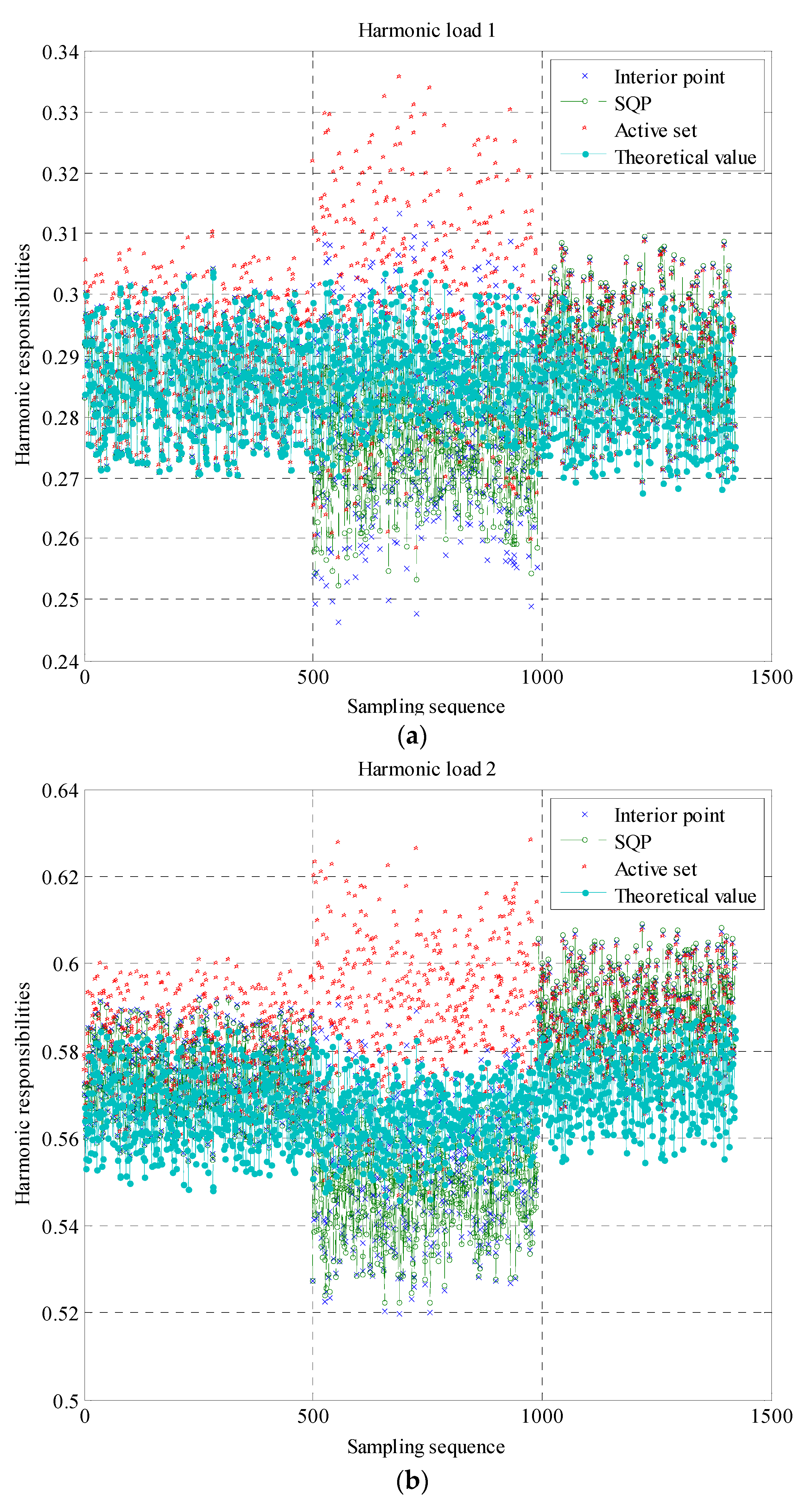
For the two harmonic loads, the harmonic responsibilities for each sample point obtained by the three algorithms are shown in Figure 5.
From the tables and figure above, the calculated values of harmonic responsibility are basically consistent with the theoretical values. For the three algorithms, the mean and the variance of the relative error are all below 0.05 and 4 × 10⁻⁴ respectively. It is evidenced that the piecewise bound constrained optimization model with the three algorithms can assess the harmonic responsibility of harmonic load accurately. In addition, compared with the AS algorithm, the results of IP and SQP algorithms are closer to the theoretical values.
In order to examine how the fluctuation of the harmonic data can affect the three algorithms, the harmonic responsibilities are evaluated while the variances of the load harmonic impedances are set within the range of 0.005 to 0.1. The calculated values of the harmonic responsibilities obtained by the three algorithms are shown in Table 4. In comparison, the SQP algorithm can provide the most accurate and stable results.
To compare the calculation times of the three optimization algorithms, the statistic results of calculated time including the maximum values, minimum values, mean values and standard deviations of 100 consecutive runs are shown in Table 5. The results show that the AS algorithm is the fastest, while the IP algorithm is the slowest. Since the harmonic responsibility is usually assessed over a period of time, such as 24 h, the computation times of all three algorithms are acceptable.
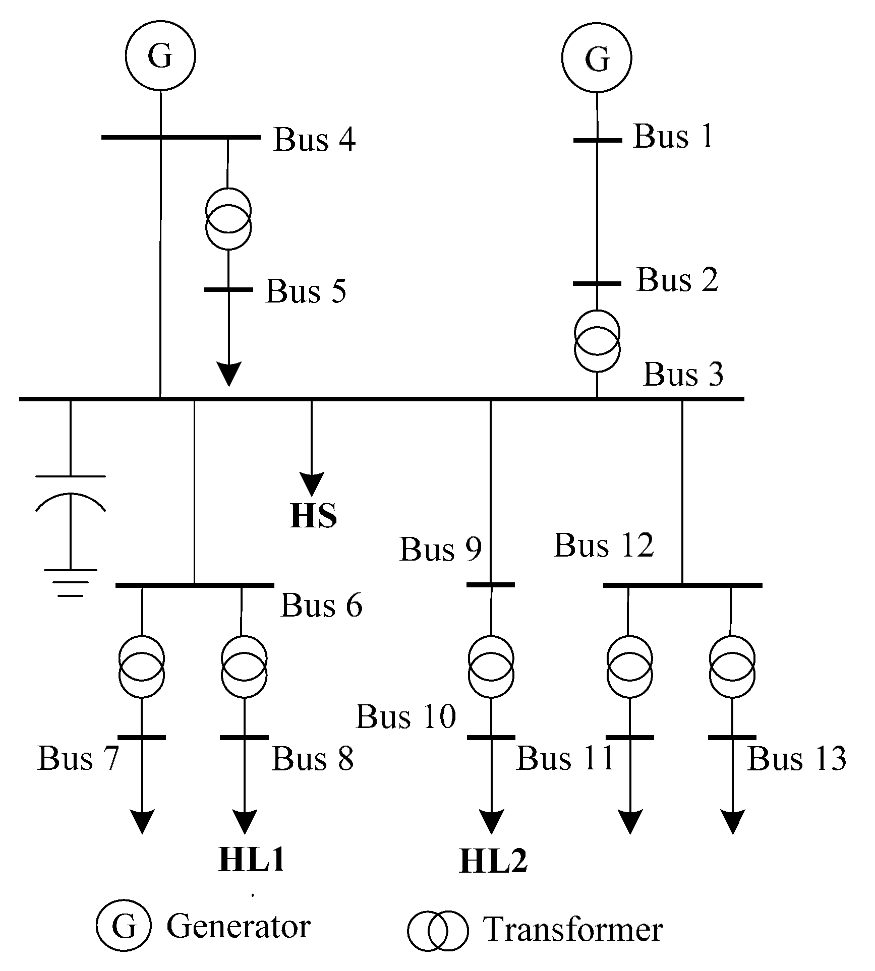
In order to further reflect the complexity of the actual distribution system, this article also carries out simulations on the IEEE 13-bus distribution system [19,32] as shown in Figure 6. The introduction of IEEE 13-bus distribution system can be seen in Appendix A.
The system parameters are referred to [32] and Table A1. In this work, the parameters of the IEEE 13-bus system are converted into the per unit values. In addition, all loads are modeled as the resistance R and reactance L in series. We take bus 3 as the bus of interest, and set load 8 and 10 as the harmonic load 1 (HL1) and harmonic load 2 (HL2), respectively. To simulate the harmonics at the utility side, the harmonic source (HS) is also injected into bus 3. In this work, the change of the reactive power compensation which can lead to the utility harmonic impedance change is analyzed.
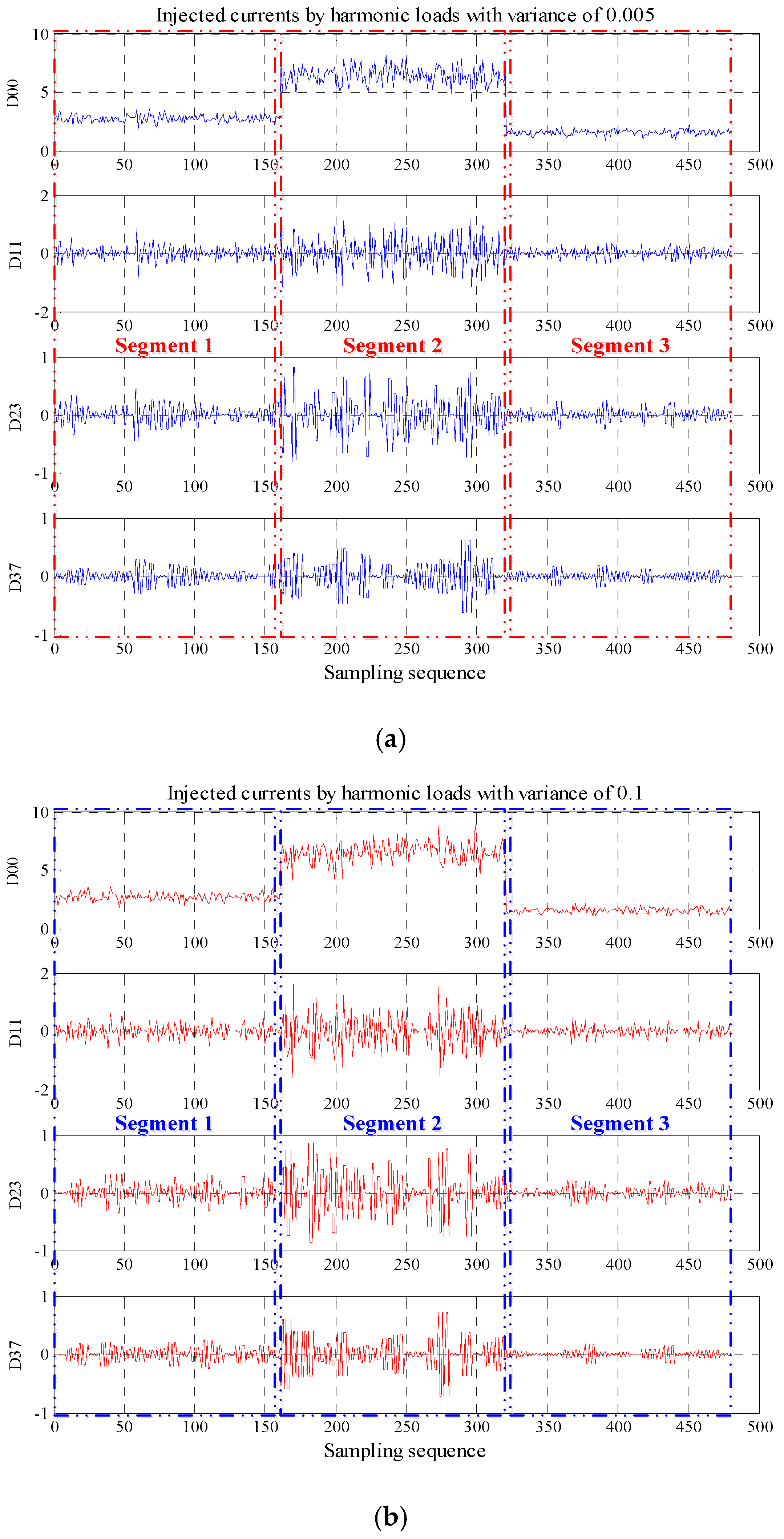
The reactive power compensation of the system is set as 4500 kvar, 5500 kvar, and 6500 kvar. As mentioned above, the variances of the injected harmonic currents are set to be 0.005 and 0.1 so as to evaluate how different data fluctuations influence the harmonic responsibility assessment. The injected harmonic currents of each bus for the two cases are shown in Table 6. The simulations of harmonic responsibility assessment are performed in MATLAB. In the simulation process, the harmonic loads are regarded as known PQ constant loads. The Newton-Raphson method [33] is used to calculate the fundamental power flow, and the injected harmonic currents are calculated according to the typical harmonic current frequency spectrum in [32]. The fifth harmonic is taken as the example for simulation.
A total of 14,400 sampling points are generated, and the reactive compensation quantity is changed for every 4800 points. The results of harmonic load flow are assumed as the measured harmonic data. In consideration of the data fluctuations in the actual system, the window length of wavelet packet transform is set to L = 30. Figure 7 presents the wavelet packet decomposition curves for the harmonic data of the two cases when a Haar wavelet is applied.
Referring to Figure 7, the change time window can be approximatively identified as 160 and 320. As the sampling window length is 30, the sampling time of the utility harmonic impedance changes is approximatively to 4800 and 9600, which is consistent with the settings of change times. Thus, the harmonic data are divided into three segments (1–4800), (4801–9600) and (9601–14,400). Then, the piecewise bound constrained optimization model, the three algorithms and the weighted summation are also utilized to compute the total harmonic responsibility for the two cases. The setting of parameters for the three algorithms, as well as the initial values and the boundary constraints have been described previously. Table 7 and Table 8 present the theoretical values and calculated values of the harmonic responsibilities obtained by the three algorithms for Case 1 and Case 2, as well as the corresponding means and variances of the relative error between the calculated value and the theoretical values.
For the segment 1 of Case 1, the convergence curves of the three algorithms are shown in Figure 8. It can be observed that the minimum objective function values obtained by IP and SQP algorithms are approximately 173, while the minimum objective function value obtained by AS algorithm is around 184. Compared to IP and SQP, the calculation error of AS algorithm is slightly larger due to the fact it is subject to the premature convergence.
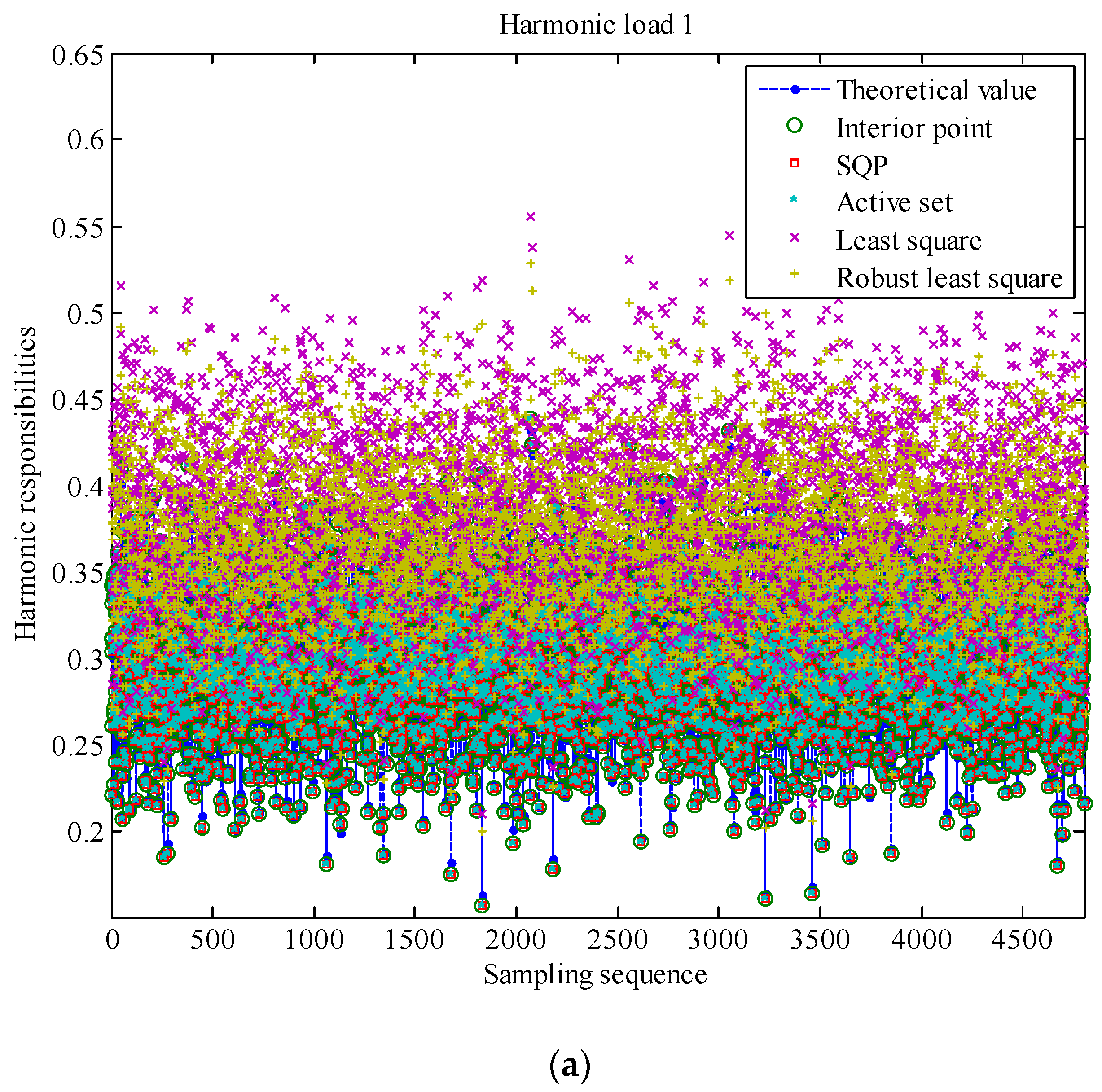
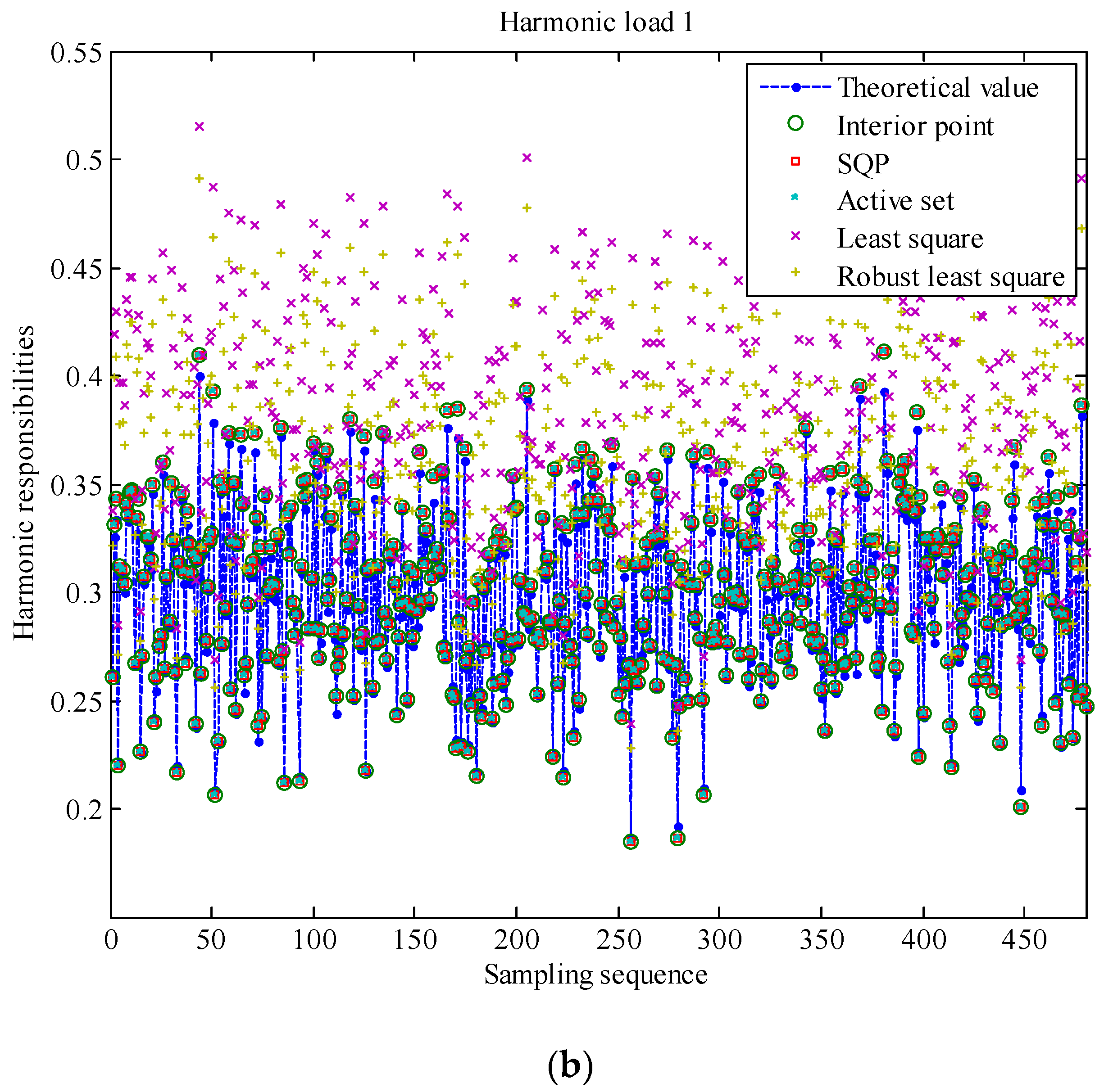
For the segment 1 of Case 2, the harmonic responsibilities for each sample point of harmonic load 1 obtained by the three algorithms are shown in Figure 9, where Figure 9a shows the results of all the 4800 sampling points, and Figure 9b shows the results of the first 480 sampling points. In order to compare with the conventional regression analysis methods, the harmonic responsibilities obtained by the least square method [12] and the robust least square method [24] are also shown in Figure 9. As shown in Figure 9, the computational accuracy of the proposed method is superior to that of least square method and robust least square method.
The results above illustrate that the proposed approach can get accurate and stable assessment results as the means and variances of the relative error are small. In addition, the calculated values obtained by the three algorithms in Case 2 are similar and close to the theoretical values, which indicate that the impacts of harmonic data fluctuation are insignificant to the three algorithms. In accordance with the test results, the IP and the SQP algorithm are recommended with the priority.
7. Conclusions
In existence of the utility harmonic impedance variations, the harmonic responsibility cannot be calculated directly using the linear regression method. Thus, this article proposes a technique for harmonic responsibility assessment by combining wavelet packet transform with piecewise bound constrained optimization approach on the condition of utility harmonic impedance changes. The first contribution lies in the determination of change times of the utility harmonic impedance by the wavelet packet transform, which aims to accurately segment the measured harmonic data according to different utility harmonic impedances. Secondly, the piecewise bound constrained optimization model is established to evaluate the harmonic responsibility of each data segment, which can provide accurate assessment results. Furthermore, the interior point, the sequential quadratic programming and the active set algorithms are utilized to solve this optimization model. Based on the results, the interior point and the sequential quadratic programming can deliver better performance compared with the active set. In the simulation process, the time variation characteristics of the harmonics have been considered. The proposed method has good robustness against the harmonic data fluctuation. Except for the measurement data of harmonic voltage and current, no additional data is required by the proposed method. The future works may focus on the adaptive modeling method for the piecewise bound constrained optimization model, which can conveniently calculate the harmonic responsibility of multiple harmonic loads.
Acknowledgments
The authors acknowledge the support by the National Natural Science Foundation for Distinguished Young Scholars of China under Grant 51525702, the National Natural Science Foundation of China under Grant 51407150, Innovative Think-tank Foundation for Young Scientists of China Association for Science and Technology under Grant DXB-ZKQN-2017-042, Open Project of Key Laboratory of electric Power Big Data of Guizhou Province and Guizhou Fengneng Science and Technology Development Co., Ltd.
Author Contributions
Tianlei Zang and Zhengyou He conceived and designed the experiments; Tianlei Zang and Yan Wang performed the experiments; Tianlei Zang and Ling Fu analyzed the data; Qingquan Qian contributed analysis tools; Tianlei Zang, Zhengyou He and Zhiyu Peng wrote the paper. All authors have read and approved the final manuscript.
Conflicts of Interest
The authors declare no conflict of interest.
Appendix A. The Introduction of IEEE 13-Bus Distribution System
The IEEE 13-bus system is a medium-sized industrial plant, which is extracted from a typical test system in the IEEE Color Book series. The system has been employed as a benchmark system to develop novel harmonic analysis approaches. The system is fed from a utility supply at 69 kV and the local distribution system operates at 13.8 kV. Because of the balanced nature of the test system, only the data of positive sequence is given. Capacitance of all cables and the short overhead lines are ignored. In addition, frequency dependence of model resistance and transformer magnetizing branch effects is ignored. The main parameters of the IEEE 13-bus distribution system are listed in Appendix Table A1.

Table A1.
The main parameters of IEEE 13-bus distribution system.
| Bus No. | Load | Bus No. | Line Impedance | Transformer Impedance | ||||
|---|---|---|---|---|---|---|---|---|
| P (p.u.) | Q (p.u.) | From | To | RL (p.u.) | XL (p.u.) | RT (p.u.) | XT (p.u.) | |
| 1 | 0.0000 | 0.0000 | 3 | 4 | 0.00122 | 0.00243 | 0.00000 | 0.00000 |
| 2 | 0.0000 | 0.0000 | 1 | 2 | 0.00139 | 0.00296 | 0.00000 | 0.00000 |
| 3 | 0.2240 | 0.2000 | 3 | 6 | 0.00075 | 0.00063 | 0.00000 | 0.00000 |
| 4 | 0.0000 | 0.0000 | 3 | 9 | 0.00157 | 0.00131 | 0.00000 | 0.00000 |
| 5 | 0.0600 | 0.0530 | 3 | 12 | 0.00109 | 0.00091 | 0.00000 | 0.00000 |
| 6 | 0.0000 | 0.0000 | 2 | 3 | 0.00000 | 0.00000 | 0.00313 | 0.05324 |
| 7 | 0.5150 | 0.8290 | 4 | 5 | 0.00000 | 0.00000 | 0.06395 | 0.37796 |
| 8 | 0.1310 | 0.1130 | 6 | 7 | 0.00000 | 0.00000 | 0.05918 | 0.35510 |
| 9 | 0.0000 | 0.0000 | 6 | 8 | 0.00000 | 0.00000 | 0.04314 | 0.34514 |
| 10 | 0.0810 | 0.0800 | 9 | 10 | 0.00000 | 0.00000 | 0.05829 | 0.37887 |
| 11 | 0.0370 | 0.0330 | 12 | 11 | 0.00000 | 0.00000 | 0.05575 | 0.36240 |
| 12 | 0.0000 | 0.0000 | 12 | 13 | 0.00000 | 0.00000 | 0.01218 | 0.14616 |
| 13 | 0.2800 | 0.2500 | ||||||
References
- Yang, N.C.; Le, M.D. Three-phase harmonic power flow by direct ZBUS method for unbalanced radial distribution systems with passive power filters. IET Gener. Transm. Distrib. 2016, 10, 3211–3219. [Google Scholar] [CrossRef]
- Zong, X.; Gray, P.A.; Lehn, P.W. New metric recommended for IEEE Standard 1547 to limit harmonics injected into distorted grids. IEEE Trans. Power Deliv. 2016, 31, 963–972. [Google Scholar] [CrossRef]
- Ye, G.; Nijhuis, M.; Cuk, V.; Cobben, J.S. Stochastic residential harmonic source modeling for grid impact studies. Energies 2017, 10, 372. [Google Scholar] [CrossRef]
- Sun, Z.M.; He, Z.Y.; Zang, T.L.; Liu, Y.L. Multi-interharmonic spectrum separation and measurement under asynchronous sampling condition. IEEE Trans. Instrum. Meas. 2016, 65, 1902–1912. [Google Scholar] [CrossRef]
- Teng, J.H.; Liao, S.H.; Leou, R.C. Three-phase harmonic analysis method for unbalanced distribution systems. Energies 2014, 7, 365–384. [Google Scholar] [CrossRef]
- Bagheri, P.B.; Xu, W.; Ding, T.Y. A distributed filtering scheme to mitigate harmonics in residential distribution systems. IEEE Trans. Power Deliv. 2016, 31, 648–656. [Google Scholar] [CrossRef]
- Pfajfar, T.; Blazic, B.; Papic, I. Harmonic contributions evaluation with the harmonic current vector method. IEEE Trans. Power Deliv. 2008, 23, 425–433. [Google Scholar] [CrossRef]
- Xu, W.; Liu, Y.L. A method for determining customer and utility harmonic contributions at the point of common coupling. IEEE Trans. Power Deliv. 2010, 15, 804–811. [Google Scholar]
- Zebardast, A.; Mokhtari, H. Technique for online tracking of a utility harmonic impedance using by synchronising the measured samples. IET Gener. Transm. Distrib. 2016, 10, 1240–1247. [Google Scholar] [CrossRef]
- Yang, H.; Pirotte, P.; Robert, A. Harmonic emission levels of industrial loads statistical assessment. In Proceedings of the International Conference on Large High Voltage Electric Systems, Paris, France, 21–26 August 1996; pp. 36–306. [Google Scholar]
- Song, K.L.; Yuan, X.D.; Chen, B.; Zhao, S. A method for assessing customer harmonic emission level based on improved fluctuation method. In Proceedings of the 2012 China International Conference on Electricity Distribution (CICED), Shanghai, China, 5–6 September 2012; pp. 1–5. [Google Scholar]
- Hui, J.; Freitas, W.; Vieira, J.C.M.; Yang, H.G.; Liu, Y.M. Utility harmonic impedance measurement based on data selection. IEEE Trans. Power Deliv. 2012, 27, 2193–2202. [Google Scholar] [CrossRef]
- Matos, E.O.D.; Soares, T.M.; Bezerra, U.H.; Tostes, M.E.D.L.; Manito, A.R.A.; Costa, B.C. Using linear and non-parametric regression models to describe the contribution of non-linear loads on the voltage harmonic distortions in the electrical grid. IET Gener. Transm. Distrib. 2016, 10, 1825–1832. [Google Scholar] [CrossRef]
- Wang, Y.; Mazin, H.E.; Xu, W.; Huang, B. Estimating harmonic impact of individual loads using multiple linear regression analysis. Int. Trans. Electr. Energy Syst. 2016, 26, 809–824. [Google Scholar] [CrossRef]
- Karimzadeh, F.; Esmaeili, S.; Hosseinian, S.H. Method for determining utility and consumer harmonic contributions based on complex independent component analysis. IET Gener. Transm. Distrib. 2016, 10, 526–534. [Google Scholar] [CrossRef]
- Zhao, X.; Yang, H.G. A new method to calculate the utility harmonic impedance based on FastICA. IEEE Trans. Power Deliv. 2016, 31, 381–388. [Google Scholar] [CrossRef]
- Hernandez, J.-C.; Ortega, M.-J.; Medina, A. Statistical characterisation of harmonic current emission for large photovoltaic plants. Int. Trans. Electr. Energy Syst. 2014, 24, 1134–1150. [Google Scholar] [CrossRef]
- Ruiz-Rodriguez, F.-J.; Hernandez, J.-C.; Jurado, F. Harmonic modelling of PV systems for probabilistic harmonic load flow studies. Int. J. Circuit Theory Appl. 2015, 43, 1541–1565. [Google Scholar] [CrossRef]
- Zang, T.L.; He, Z.Y.; Fu, L.; Wang, Y.; Qian, Q.Q. Adaptive method for harmonic contribution assessment based on hierarchical K-means clustering and Bayesian partial least squares regression. IET Gener. Transm. Distrib. 2016, 10, 3220–3227. [Google Scholar] [CrossRef]
- Shojaie, M.; Mokhtari, H. A method for determination of harmonics responsibilities at the point of common coupling using data correlation analysis. IET Gener. Transm. Distrib. 2014, 8, 142–150. [Google Scholar] [CrossRef]
- Kandev, N.P.; Chenard, S. Method for determining customer contribution to harmonic variations in a large power network. In Proceedings of the 14th International Conference on Harmonics and Quality of Power (ICHQP 2010), Bergamo, Italy, 26–29 September 2010. [Google Scholar]
- Mehrasa, M.; Pouresmaeil, E.; Akorede, M.F.; Jørgensen, B.N.; Catalão, J.P. Multilevel converter control approach of active power filter forharmonics elimination in electric grids. Energy 2015, 84, 722–731. [Google Scholar] [CrossRef]
- Godina, R.; Rodrigues, E.; Pouresmaeil, E.; Matias, J.C.O.; Catalão, J.P.S. Model predictive control technique for energy optimization in residential sector. In Proceedings of the 16th IEEE International Conference on Environment and Electrical Engineering (EEEIC 2016), Florence, Italy, 7–10 June 2016. [Google Scholar]
- Sun, Y.Y.; Li, J.Q.; Yin, Z.M. Quantifying harmonic impacts for concentrated multiple harmonic sources using actual data. Proc. Chin. Soc. Electr. Eng. 2014, 34, 2164–2171. [Google Scholar]
- Do, H.T.; Zhang, X.; Nguyen, N.V.; Li, S.S.; Chu, T. Passive-islanding detection method using the wavelet packet transform in grid-connected photovoltaic systems. IEEE Trans. Power Electr. 2015, 31, 6955–6967. [Google Scholar] [CrossRef]
- Hazewinkel, M. Encyclopaedia of Mathematics: Cosine Theorem; Springer: Berlin/Heidelberg, Germany, 2001. [Google Scholar]
- Morini, B.; Simoncini, V.; Tani, M. Spectral estimates for unreduced symmetric KKT systems arising from Interior Point methods. Numer. Linear Algebra Appl. 2016, 23, 776–800. [Google Scholar] [CrossRef]
- Izmailov, A.F.; Solodov, M.V.; Uskov, E.I. Globalizing stabilized sequential quadratic programming method by smooth primal-dual exact penalty function. J. Optim. Theory Appl. 2016, 169, 148–178. [Google Scholar] [CrossRef]
- Buerger, J.; Cannon, M.; Kouvaritakis, B. Active set solver for min-max robust control with state and input constraints. Int. J. Robust Nonlinear Control 2016, 26, 3209–3231. [Google Scholar] [CrossRef]
- Coleman, T.; Branch, M.; Grace, A. Optimization Toolbox for Use with MATLAB, User’s Guide; Version 3; MathWorks: Natick, MA, USA, 1999. [Google Scholar]
- Urban, K. Wavelets in Numerical Simulation: Wavelet Bases; Springer: Berlin/Heidelberg, Germany, 2002; pp. 1–81. [Google Scholar]
- Abu-Hashim, R.; Burch, R.; Chang, G.; Grady, M.; Gunther, E.; Halpin, M.; Harziadonin, C.; Liu, Y.; Marz, M.; Ortmeyer, T. Test systems for harmonics modeling and simulation. IEEE Trans. Power Deliv. 1999, 14, 579–587. [Google Scholar] [CrossRef]
- Costa, V.M.D.; Martins, N.; Pereira, J.L.R. Developments in the Newton Raphson power flow formulation based on current injections. IEEE Trans. Power Syst. 1999, 14, 1320–1326. [Google Scholar] [CrossRef]
Figure 1.
A typical distribution system with two major harmonic loads and its harmonic voltage phasors: (a) The Norton equivalent circuit; (b) Phasor diagram of the h-th harmonic voltages.
Figure 1.
A typical distribution system with two major harmonic loads and its harmonic voltage phasors: (a) The Norton equivalent circuit; (b) Phasor diagram of the h-th harmonic voltages.

Figure 2.
Wavelet packet decomposition tree with three decomposition levels.
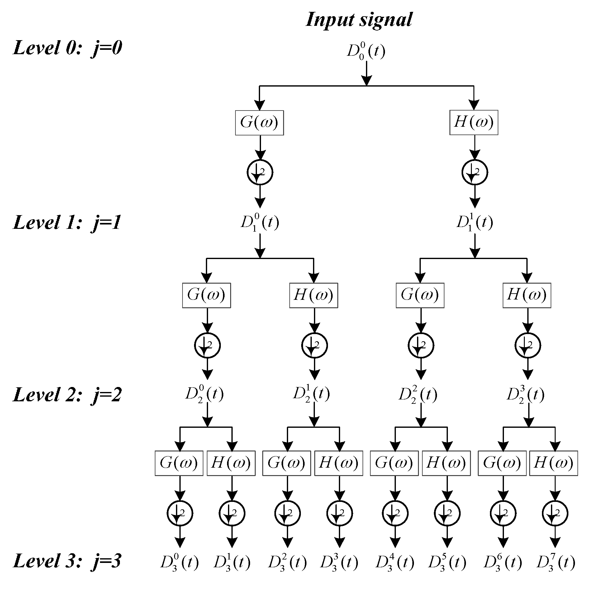
Figure 3.
The process of the proposed approach.

Figure 4.
Wavelet packet decomposition curves: (a) Wavelet packet decomposition curves of the utility harmonic impedance rough estimation values; (b) The three concerned high frequency components.
Figure 4.
Wavelet packet decomposition curves: (a) Wavelet packet decomposition curves of the utility harmonic impedance rough estimation values; (b) The three concerned high frequency components.

Figure 5.
The harmonic responsibilities for each sample point of harmonic loads: (a) The harmonic responsibilities of load 1; (b) The harmonic responsibilities of load 2.
Figure 5.
The harmonic responsibilities for each sample point of harmonic loads: (a) The harmonic responsibilities of load 1; (b) The harmonic responsibilities of load 2.

Figure 6.
IEEE 13-bus distribution system.

Figure 7.
The wavelet packet decomposition curves for the harmonic data of the two cases: (a) The Case 1; (b) The Case 2.
Figure 7.
The wavelet packet decomposition curves for the harmonic data of the two cases: (a) The Case 1; (b) The Case 2.

Figure 8.
The convergence curves of the three algorithms.
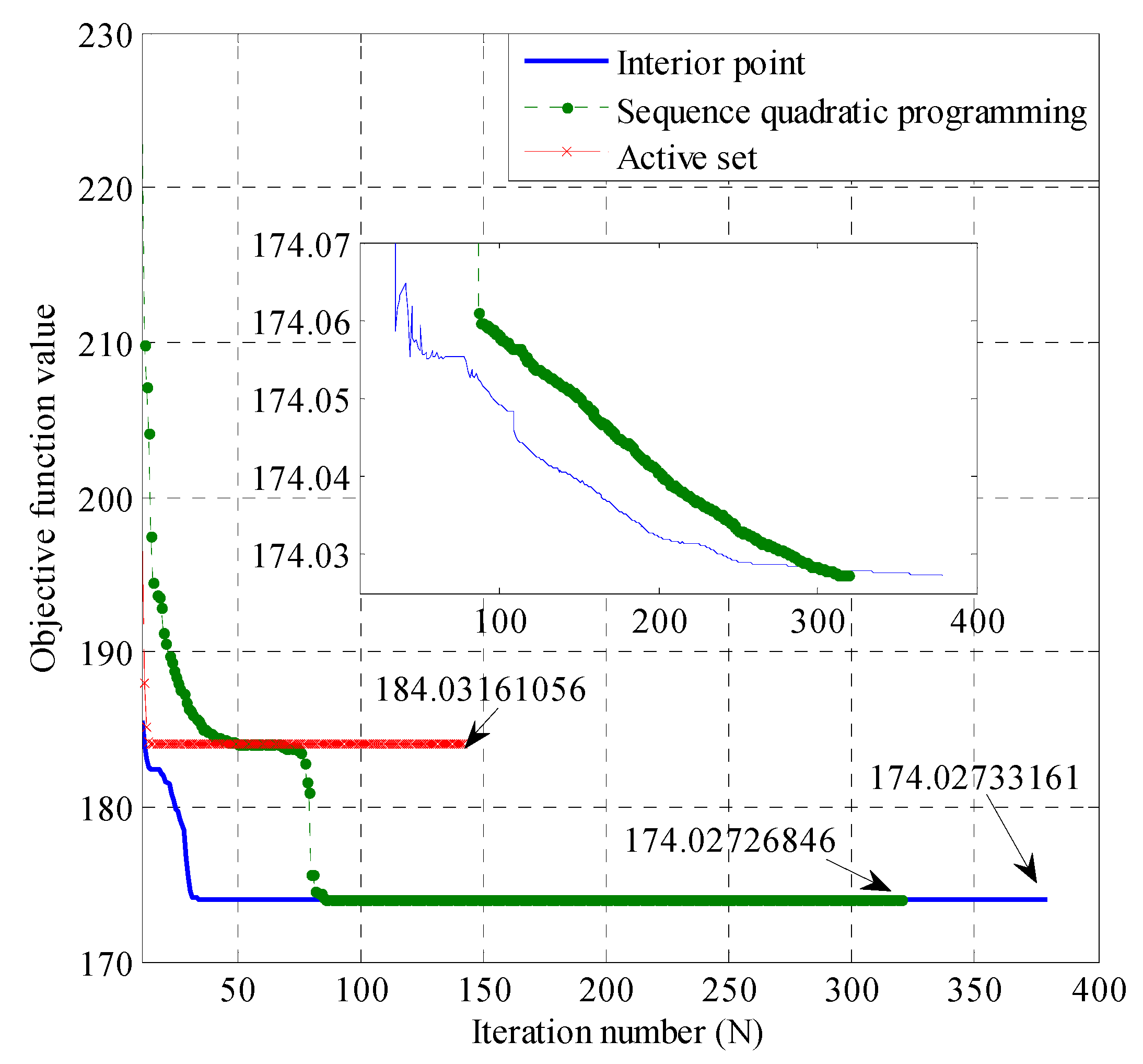
Figure 9.
The harmonic responsibilities for each sample point of harmonic load 1: (a) The results of all the 4800 sampling points; (b) The results of the first 480 sampling points.
Figure 9.
The harmonic responsibilities for each sample point of harmonic load 1: (a) The results of all the 4800 sampling points; (b) The results of the first 480 sampling points.


Table 1.
Parameter values of the distribution system Norton equivalent circuit.
| Parameters | Values (Ω) | The Numbers of Sampling Points |
|---|---|---|
| 500 | ||
| 500 | ||
| 1440 | ||
| 1440 | ||
| 1440 |
Table 2.
Identification results of the change time windows of utility harmonic impedance under different wavelet bases.
Table 2.
Identification results of the change time windows of utility harmonic impedance under different wavelet bases.
| Wavelet Basis | Identified Change Time Window | Actual Change Time Window |
|---|---|---|
| haar (db1), sym1 | 167 168 333 334 335 336 | 167 334 |
| db4 | 166 167 333 334 335 336 337 | |
| sym4 | 168 331 332 333 334 335 336 338 | |
| coif4 | 167 330 331 333 334 335 336 337 339 | |
| dmey | 167 331 333 334 335 337 |
Table 3.
The harmonic responsibilities obtained by the three algorithms and error statistics.
| Segment No. | Algorithm | Harmonic Responsibility of Load 1 | Harmonic Responsibility of Load 2 | ||||||
|---|---|---|---|---|---|---|---|---|---|
| Theoretical Value (%) | Calculated Value (%) | The mean of the Relative Error | The Variance of the Relative Error | Theoretical Value (%) | Calculated Value (%) | The Mean of the Relative Error | The Variance of the Relative Error | ||
| 1 | IP | 28.61 | 28.63 | 1.07 × 10⁻³ | 6.45 × 10⁻⁷ | 56.73 | 57.40 | 1.18 × 10⁻² | 9.21 × 10⁻⁷ |
| SQP | 28.61 | 9.12 × 10⁻⁴ | 4.20 × 10⁻⁷ | 57.36 | 1.11 × 10⁻² | 9.41 × 10⁻⁷ | |||
| AS | 28.96 | 1.22 × 10⁻² | 1.53 × 10⁻⁵ | 58.05 | 2.32 × 10⁻² | 3.32 × 10⁻⁶ | |||
| 2 | IP | 28.72 | 27.92 | 3.10 × 10⁻² | 3.90 × 10⁻⁴ | 56.44 | 55.51 | 1.75 × 10⁻² | 1.28 × 10⁻⁴ |
| SQP | 2760 | 3.91 × 10⁻² | 1.16 × 10⁻⁴ | 54.84 | 2.85 × 10⁻² | 3.90 × 10⁻⁵ | |||
| AS | 29.55 | 3.39 × 10⁻² | 5.63 × 10⁻⁴ | 58.75 | 4.06 × 10⁻² | 2.34 × 10⁻⁴ | |||
| 3 | IP | 28.37 | 28.88 | 1.78 × 10⁻² | 2.15 × 10⁻⁵ | 57.28 | 58.75 | 2.56 × 10⁻² | 3.91 × 10⁻⁶ |
| SQP | 28.91 | 1.89 × 10⁻² | 2.36 × 10⁻⁵ | 58.81 | 2.67 × 10⁻² | 4.33 × 10⁻⁶ | |||
| AS | 28.86 | 1.70 × 10⁻² | 1.89 × 10⁻⁵ | 58.70 | 2.47 × 10⁻² | 3.39 × 10⁻⁶ | |||
| Total | IP | 28.58 | 28.46 | 1.65 × 10⁻² | 2.98 × 10⁻⁴ | 56.80 | 57.16 | 1.80 × 10⁻² | 7.67 × 10⁻⁵ |
| SQP | 28.35 | 1.96 × 10⁻² | 3.01 × 10⁻⁴ | 56.93 | 2.19 × 10⁻² | 7.77 × 10⁻⁵ | |||
| AS | 29.13 | 2.12 × 10⁻² | 2.96 × 10⁻⁴ | 58.49 | 2.97 × 10⁻² | 1.46 × 10⁻⁴ | |||
Table 4.
The harmonic responsibilities under different variances of the load harmonic impedances.
| Variance of Load Harmonic Impedances | Algorithm | Harmonic Responsibility of Load 1 | Harmonic Responsibility of Load 1 | ||
|---|---|---|---|---|---|
| Calculated Value (%) | Theoretical Value (%) | Calculated Value (%) | Theoretical Value (%) | ||
| 0.005 | IP | 29.27 | 28.58 | 58.53 | 56.80 |
| SQP | 28.49 | 56.97 | |||
| AS | 29.24 | 58.47 | |||
| 0.010 | IP | 29.54 | 28.58 | 59.22 | 56.80 |
| SQP | 28.39 | 56.95 | |||
| AS | 29.40 | 58.93 | |||
| 0.050 | IP | 29.76 | 28.58 | 59.83 | 56.80 |
| SQP | 29.42 | 59.14 | |||
| AS | 29.39 | 59.08 | |||
| 0.100 | IP | 29.00 | 28.58 | 58.04 | 56.80 |
| SQP | 28.52 | 57.09 | |||
| AS | 28.94 | 57.93 | |||
Table 5.
The calculated time statistic results of the three optimization algorithms.
| Algorithms | Statistical Value of Calculation Times | |||
|---|---|---|---|---|
| Maximum Values (s) | Minimum Values (s) | Mean Values (s) | Standard Deviations | |
| IP | 38.6060 | 32.1420 | 33.9347 | 1.1632 |
| SQP | 4.3210 | 3.5920 | 3.8050 | 0.1344 |
| AS | 2.6990 | 2.2150 | 2.3595 | 0.0986 |
Table 6.
The injected harmonic current for the two cases.
| Case | Injected Bus | Injected Harmonic Current | |
|---|---|---|---|
| Mean (p.u.) | Variance | ||
| Case 1 | 3 | I3 = 0.6073 − j0.8896 | 0.005 |
| 8 | I8 = 1.1757 − j1.7222 | ||
| 10 | I10 = 2.2429 − j3.2855 | ||
| Case 2 | 3 | I3 = 0.6324 − j0.9263 | 0.100 |
| 8 | I8 = 1.1877 − j1.7398 | ||
| 10 | I10 = 2.2482 − j3.2932 | ||
Table 7.
The harmonic responsibilities and error statistics (Case 1).
| Segment No. | Algorithm | Harmonic Responsibility of Load 1 | Harmonic Responsibility of Load 2 | ||||||
|---|---|---|---|---|---|---|---|---|---|
| Theoretical Value (%) | Calculated Value (%) | The Mean of the Relative Error | The Variance of the Relative Error | Theoretical Value (%) | Calculated Value (%) | The Mean of the Relative Error | The Variance of the Relative Error | ||
| 1 | IP | 29.84 | 30.78 | 3.12 × 10⁻² | 2.03 × 10⁻⁴ | 55.51 | 55.71 | 7.09 × 10⁻³ | 2.85 × 10⁻⁵ |
| SQP | 30.77 | 3.11 × 10⁻² | 2.04 × 10⁻⁴ | 55.70 | 7.06 × 10⁻³ | 2.83 × 10⁻⁵ | |||
| AS | 33.48 | 1.22 × 10⁻¹ | 1.02 × 10⁻⁴ | 66.50 | 1.98 × 10⁻¹ | 2.95 × 10⁻⁵ | |||
| 2 | IP | 29.86 | 30.12 | 8.77 × 10⁻³ | 2.44 × 10⁻⁶ | 55.52 | 56.19 | 1.21 × 10⁻² | 2.51 × 10⁻⁶ |
| SQP | 29.95 | 3.17 × 10⁻³ | 2.48 × 10⁻⁶ | 55.87 | 6.43 × 10⁻³ | 2.64 × 10⁻⁶ | |||
| AS | 30.31 | 1.53 × 10⁻¹ | 2.26 × 10⁻⁶ | 56.55 | 1.86 × 10⁻² | 2.27 × 10⁻⁶ | |||
| 3 | IP | 29.83 | 30.26 | 1.43 × 10⁻² | 2.99 × 10⁻⁶ | 55.53 | 55.17 | 6.42 × 10⁻³ | 2.87 × 10⁻⁶ |
| SQP | 30.24 | 1.36 × 10⁻² | 3.02 × 10⁻⁶ | 55.13 | 7.12 × 10⁻³ | 2.90 × 10⁻⁶ | |||
| AS | 30.24 | 1.36 × 10⁻² | 3.02 × 10⁻⁶ | 55.13 | 7.12 × 10⁻³ | 2.90 × 10⁻⁶ | |||
| Total | IP | 29.84 | 30.38 | 1.81 × 10⁻² | 1.61 × 10⁻⁴ | 55.52 | 55.69 | 8.53 × 10⁻³ | 1.77 × 10⁻⁵ |
| SQP | 30.32 | 1.59 × 10⁻² | 2.02 × 10⁻⁴ | 55.57 | 6.87 × 10⁻³ | 1.14 × 10⁻⁵ | |||
| AS | 31.34 | 5.02 × 10⁻² | 2.59 × 10⁻³ | 59.39 | 7.45 × 10⁻² | 7.63 × 10⁻³ | |||
Table 8.
The harmonic responsibilities and error statistics (Case 2).
| Segment No. | Algorithm | Harmonic Responsibility of Load 1 | Harmonic Responsibility of Load 2 | ||||||
|---|---|---|---|---|---|---|---|---|---|
| Theoretical Value (%) | Calculated Value (%) | The Mean of the Relative Error | The Variance of the Relative Error | Theoretical Value (%) | Calculated Value (%) | The Mean of the Relative Error | The Variance of the Relative Error | ||
| 1 | IP | 29.822026 | 30.082117 | 1.13 × 10⁻² | 7.12 × 10⁻⁵ | 55.184464 | 55.330464 | 6.04 × 10⁻³ | 3.65 × 10⁻⁵ |
| SQP | 30.081910 | 1.12 × 10⁻² | 7.11 × 10⁻⁵ | 55.330081 | 6.04 × 10⁻³ | 3.65 × 10⁻⁵ | |||
| AS | 30.081926 | 1.12 × 10⁻² | 7.11 × 10⁻⁵ | 55.330075 | 6.04 × 10⁻³ | 3.65 × 10⁻⁵ | |||
| 2 | IP | 29.792924 | 32.418823 | 8.72 × 10⁻² | 1.20 × 10⁻⁴ | 55.226745 | 59.116948 | 7.40 × 10⁻³ | 5.48 × 10⁻⁵ |
| SQP | 32.418871 | 8.72 × 10⁻² | 1.20 × 10⁻⁴ | 59.117040 | 7.40 × 10⁻³ | 5.48 × 10⁻⁵ | |||
| AS | 32.418872 | 8.72 × 10⁻² | 1.20 × 10⁻⁴ | 59.117016 | 7.40 × 10⁻³ | 5.48 × 10⁻⁵ | |||
| 3 | IP | 29.828965 | 30.810225 | 3.32 × 10⁻² | 4.03 × 10⁻⁵ | 55.172325 | 57.453403 | 6.40 × 10⁻³ | 4.10 × 10⁻⁵ |
| SQP | 30.814266 | 3.34 × 10⁻² | 4.03 × 10⁻⁵ | 57.460951 | 6.40 × 10⁻³ | 4.09 × 10⁻⁵ | |||
| AS | 30.814327 | 3.34 × 10⁻² | 4.03 × 10⁻⁵ | 57.461059 | 6.40 × 10⁻³ | 4.09 × 10⁻⁵ | |||
| Total | IP | 29.814638 | 31.103722 | 4.39 × 10⁻² | 1.09 × 10⁻³ | 55.194512 | 57.300272 | 3.98 × 10⁻² | 7.03 × 10⁻⁴ |
| SQP | 31.105015 | 4.39 × 10⁻² | 1.09 × 10⁻³ | 57.302691 | 3.98 × 10⁻² | 7.03 × 10⁻⁴ | |||
| AS | 31.105042 | 4.39 × 10⁻² | 1.09 × 10⁻³ | 57.302717 | 3.98 × 10⁻² | 7.03 × 10⁻⁴ | |||
© 2017 by the authors. Licensee MDPI, Basel, Switzerland. This article is an open access article distributed under the terms and conditions of the Creative Commons Attribution (CC BY) license (http://creativecommons.org/licenses/by/4.0/).
Share and Cite
MDPI and ACS Style
Zang, T.; He, Z.; Wang, Y.; Fu, L.; Peng, Z.; Qian, Q. A Piecewise Bound Constrained Optimization for Harmonic Responsibilities Assessment under Utility Harmonic Impedance Changes. Energies 2017, 10, 936. https://doi.org/10.3390/en10070936
AMA Style
Zang T, He Z, Wang Y, Fu L, Peng Z, Qian Q. A Piecewise Bound Constrained Optimization for Harmonic Responsibilities Assessment under Utility Harmonic Impedance Changes. Energies. 2017; 10(7):936. https://doi.org/10.3390/en10070936
Chicago/Turabian StyleZang, Tianlei, Zhengyou He, Yan Wang, Ling Fu, Zhiyu Peng, and Qingquan Qian. 2017. "A Piecewise Bound Constrained Optimization for Harmonic Responsibilities Assessment under Utility Harmonic Impedance Changes" Energies 10, no. 7: 936. https://doi.org/10.3390/en10070936
Note that from the first issue of 2016, this journal uses article numbers instead of page numbers. See further details here.