1. Introduction
A major challenge in Smart Cities (SC) [
1] is the dynamic optimization of routes under different criteria. The objective is to manage a flood of electrical vehicles (EV) efficiently and in a sustainable way. This also implies finding the correct position of charging stations and the optimization of routes to recharge the electric vehicles.
The problem can be solved using different strategies. A popular method found in the literature is the vehicle routing problem (VRP) [
2]. This problem was introduced by Dantzig and Ramser in 1959. There, the authors found a mathematical solution to the problem of gas distribution among different gas stations [
3]. However, the limited battery capacities of EVs required a new approach. In 2011 Conrad and Figliozzi presented a new variant; the problem of vehicle routing recharge (RVRP), which includes the management of charging and discharging times. Combining the problem with a multi-agent architecture is shown to provide good results [
4]. In [
5,
6] the authors present different types of hybrid heuristics to solve the electric vehicle-routing problem with time windows and charging stations. However, none of these works considers the problem of finding a charging station in case of partial information. In this setting, we can find a damaged recharge station, a new recharge station which has not been added to the system, or a station which uses a different type of plug, that is not suitable for the type of the vehicle. Some problems related to the environment can also occur, such as traffic congestion or sudden interruptions on the road. A solution to this problem can be found in [
7]. In these cases, we cannot rely on this information and we have to explore the environment in order to find new recharge stations.
The main difficulty in this case is to avoid traveling over the same paths. As we show in this paper this problem can be solved by implementing a mechanism that leaves bread crumbs (e.g., messages) on the path. This behavior has been termed as implicit/indirect communication in previous works. Implicit communication—also known as stigmergy—is based on the context and its most typical applications can be found in [
8,
9,
10,
11]. In this regard, the pioneer work of Pierre-Paul Grasse in termite colonies revealed the communication mechanisms of these insects by means of chemical signaling and in particular by pheromones [
12]. These observations resulted in an ant-based exploration algorithm [
13]. Here, each ant leaves a pheromone trail in its foraging activity. This trail persists for some time and it is followed by other ants in the search of food resources.
Also, the pheromone approach has been widely adapted to several artificial intelligence problems in its converse flavor (i.e., anti-pheromones) [
14,
15,
16]. In particular, some researchers have used anti-pheromone (APH) proxies to optimize robot exploration [
17]. The main advantage is that each unit accesses a different region fostering the diversity of the solutions by means of indirect and decentralized communication.
On the other hand, the efficient exploration and target localization in urban environments is gaining more and more attention [
18,
19]. However, bio-inspired algorithms tailored to optimize robot exploration and dynamic route generation in SC are somewhat separate research fields.
Moreover, RVRP solutions only work if the locations of the charging stations is known beforehand. Therefore, it is necessary to come up with a new solution for cases where the position of the charging stations cannot be known or if it is inaccurate. This solution should also enable us to find target locations in the shortest time possible. In this work, we propose an APH-based strategy aimed at optimizing these routing times in presence of uncertainty. A simple Markov model will also provide insight into the local rules that produce the observed behaviour at a large time scale.
This paper is organized as follows. In
Section 2.1 we present the APH-based algorithm. We explore numerically this strategy in a synthetic lattice in
Section 2.2 and we validate the approach through an experiment campaign with prototypes in
Section 2.3. In
Section 2.4, we introduce the perturbed Markov chain model. Finally, in
Section 2.5 we apply the algorithm to real urban environments. The main outcomes from this study are summarized in
Section 3 and we conclude in
Section 4.
2. Materials and Methods
To test the feasibility of the presented algorithm we will use a setting in which an EV has to find a recharge station. The EV has a map with partial information, with which it can get to know the topology of the environment but not the position of the recharge station. The map is static; the configuration of the routes and the positions of the recharge stations cannot change during the experiment. Also, we do not consider the traffic jam problem or other environment constraints.
The use of EVs makes it necessary to consider the capacity of the batteries. Usually, this aspect is modeled with the discharge rate of the battery or the maximum time limit. In our case, we do not consider this aspect explicitly, however, we do use a secondary parameter, called “arrival time”. The goal is to avoid the battery form discharging completely, we can deduce that in this problem it is necessary to minimize the time it takes to find a recharge station. In this way, we only need to use one parameter to model the problem.
In order to validate our approach the first step is to simulate the APH algorithm in a grid. The simulation consists of an EV traveling through a square lattice which tries to find a charging station in the shortest time possible. This type of map adds a restriction in which the EVs can only circulate through the grid lines and not in whichever direction. This corresponds to the reality, in which an EV can only circulate on the roads. Here we conduct a statistical analysis of the parameters involved in order to reduce the time of finding the charging station. In the next phase we test the results obtained in the simulation in a real EV. The experimental set-up consists of a robot prototype designed in the electronics laboratory of the University of Salamanca navigating over a printed poster grid. We measured the empirical travel times to the target and then we compared the results with our simulations.
From the analysis of both the simulation and the experiment datasets we built a theoretical model that enables us to explain the observed behavior. This is a modification of a lattice Markov Chain process where a subset of perturbing sources creates an asymmetry in the random walk transition probabilities as we discuss below.
Finally, we conducted numerical simulations using the bicycle paths of four Spanish cities; Gijon, Castellon, Barcelona and Madrid. We verify that the large scale behavior is the same as in the synthetic environment used in the laboratory experiments. In the following we provide a more detailed description of our approach.
2.1. An Anti-Pheromone Navigation Based Algorithm
The navigation algorithm we present in this work (pseudocode in Algorithm 1) is an adaptation of the classical two-dimensional APH gradient [
18] to a 1D gridded world. This world consists of a set of parallel and perpendicular lines arranged in a way that mimics urban topologies with a Manhattan distance.
| Algorithm 1 Anti-pheromone navigation algorithm. |
- 1:
procedure APH - 2:
while current_location ≠ target do - 3:
if current_location = intersection then - 4:
[paths] ← getPaths( ) - 5:
angle ← getRandomPath([paths]) - 6:
turn ( angle ) - 7:
go on - 8:
else if current_location = dead_end then - 9:
turn ( ) - 10:
else - 11:
drop anti-pheromone - 12:
go on
|
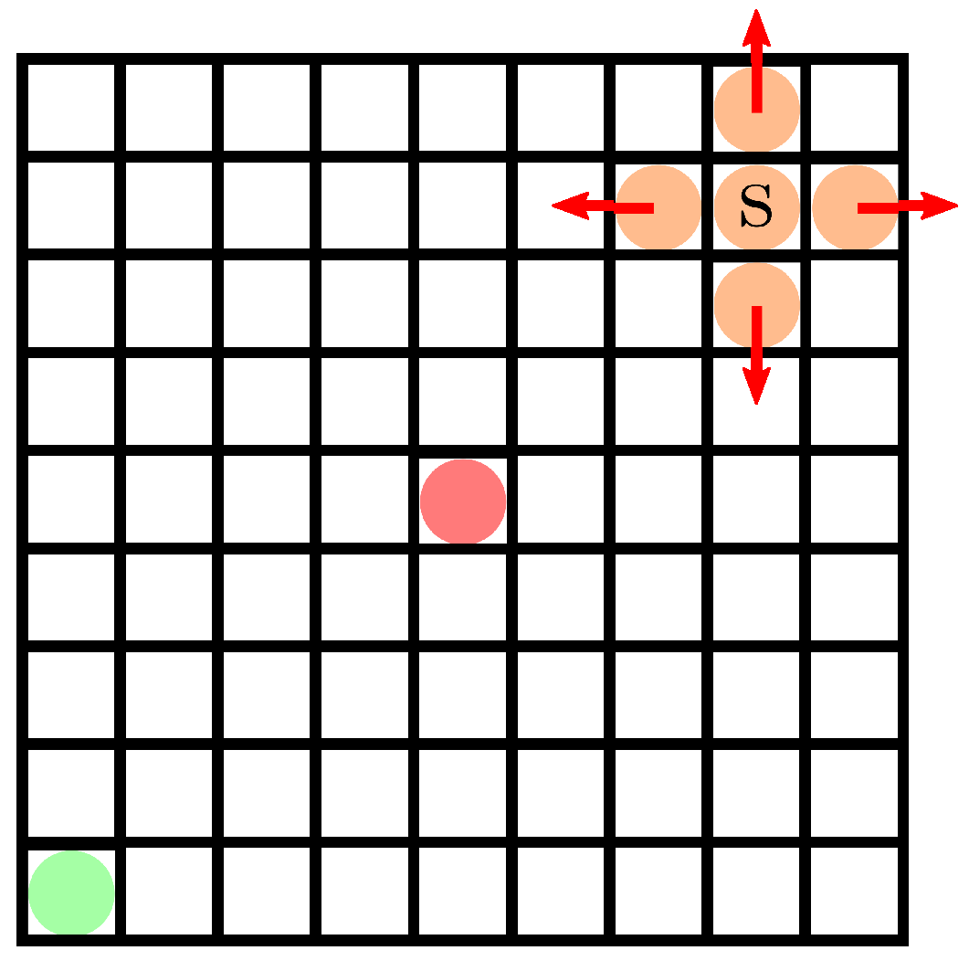
Our electric vehicle is designed to mimic the behaviour of an insect. The EV moves along a path until it reaches an intersection. At every step it leaves a unit of anti-pheromone. At the intersection the EV decides which path must be followed. The selected path is that with the lowest amount of anti-pheromones (see getPaths() in Algorithm 1). In cases where two or more paths have the same number of anti-pheromones, one of the paths is chosen at random (see getRandomPath() in Algorithm 1). This way we use a greedy strategy for every local routing decision. The execution of the algorithm finishes when the vehicle finds a recharge station, this way avoiding the exploration of the entire environment.
This algorithm enables us to explore the map in a pseudorandomized way. Whenever possible, traveling over the same path is avoided. It is also avoided that the EV gets trapped in a local minimum; as the number of anti-pheromones increases, repulsion also increases and the tendency is to dive into unexplored regions. We considered a local minimum as a loop in the map.
This approach can be easily extended for the case of multiple electric vehicles. In this case, each EV would explore a different area of the map and would prevent the other vehicles from exploring these areas. Once a position is found, this information is then broadcast to the rest of the vehicles. It can also be adapted to a random number of available recharge stations from where a target subset can be chosen.
In the following section we apply this strategy to different scenarios.
2.2. Numerical Simulations with a Synthetic Grid Map
Our tests consists of an gridded world. In this setting we define the following parameters:
n: number of EVs
: proportion of path units with respect to the total number of cells. This provides a measure for the spatial complexity of the map. In this case we obtained a complexity of .
: pheromone evaporation time (i.e., number of time units a pheromone takes to evaporate). At every time step the EVs leave a pheromone unit.
For the simulation we ran a parameter sweep with , and with . Every combination of parameters has been repeated 500 times for the statistical analysis. The target and initial position are located the closest possible to the center of the map and to the southwest corner respectively. At each run we obtained the arrival times to the target t.
2.3. Experiment with Robot Prototypes
In this phase we conduct empirical experiments with a real EV. To this end we built real robot prototypes to monitor the APH navigation strategy in the laboratory. The reason for using real robots is that these prototypes—as electric vehicles—are subjected to incidents which can be extrapolated to the incidents that are commonly found in real EV scenarios. The use of robots entails an intrinsic need to handle some errors, such as failures in communications, running off track, acceleration and turning time errors, loss of power when the battery levels drop, etc. The errors that we notice in small vehicles can be extrapolated to failures in real EVs as can be seen in
Table 1. In this work we assume that the difference between the errors made by the robot and those made by EVs is acceptable in the experimentation phase in a laboratory.
In particular, position measurement errors and communication inaccuracies found in real environments also occur in the prototypes. Moreover, the lab tests allow us to explore the robustness of our approach, which is a major concern in real robotic implementations.
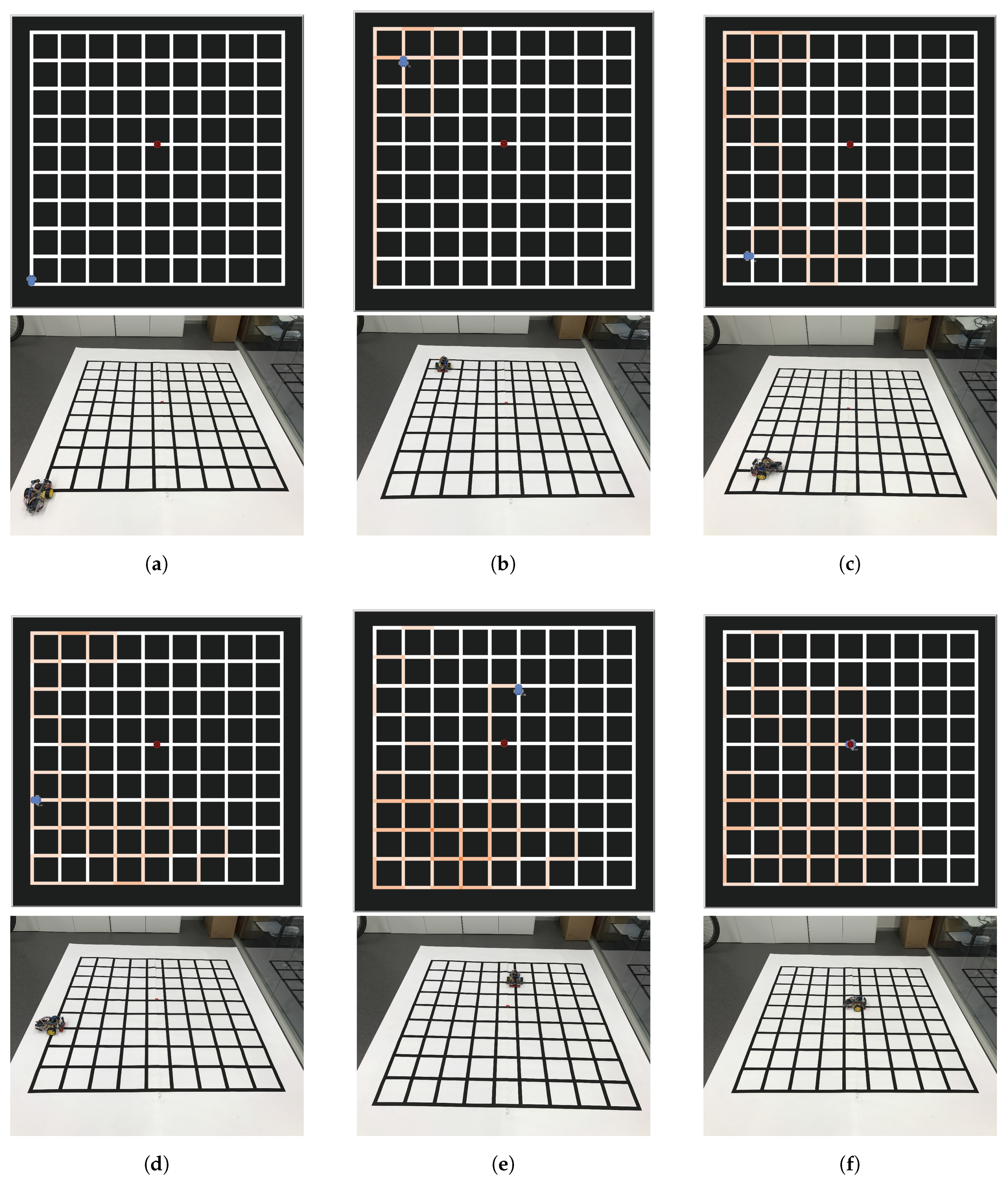
The map consist of straight black lines printed on a 2 m × 2 m white surface. The map was scaled so that each 2 cm × 2 cm corresponds to a cell unit in the simulated environment. The robot uses the Message Queue Telemetry Transport (MQTT) protocol for the communication between the robot and the software.
During the exploration the robot sends an MQTT message through Wi-Fi, for every 2 cm traveled. The robot stops when it reaches an intersection. There, it sends another MQTT message and waits for a response to determine its next move. An agent-based software receives all these messages and updates the pheromone information. Then, the software counts the current APH level of all the possible paths and it choses the path with the lowest APH level. Finally it sends back an MQTT message to the robot.
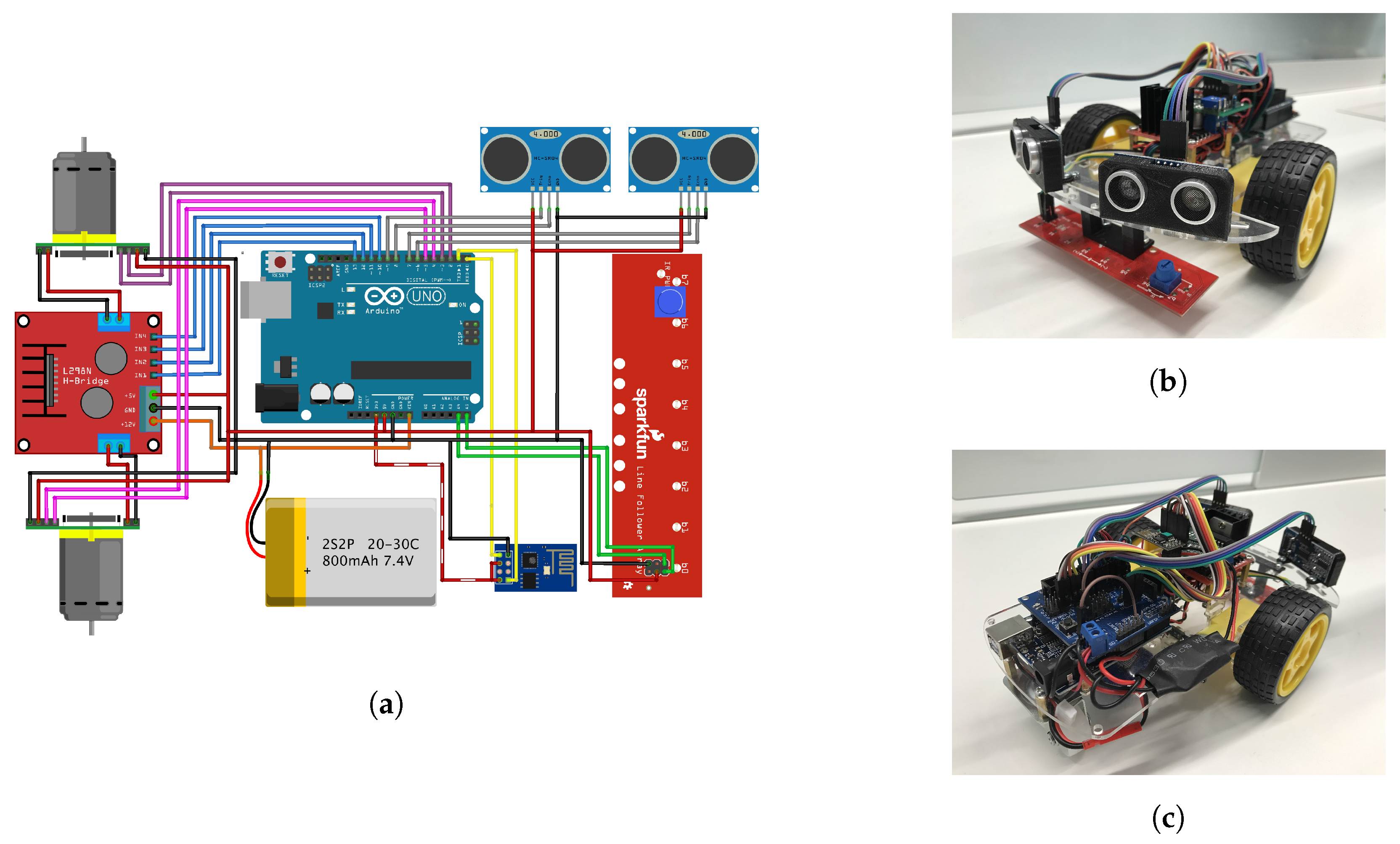
The prototype -Pyxis- has been constructed and tested by the electronics section of the BISITE research group at the University of Salamanca (
Figure 1). An Arduino UNO board is used as a microcontroller. The motors’ control is enhanced through a driver based on the chip L298n. Wi-Fi communication is enabled through an ESP8266 board. The robot holds a 2 cell Lithium 800 mAh based battery.
The sensing system of the robot consists of the following three parts:
An I2C line follower array; a long board of eight infrared sensors configured to be read as digital bits.
Two ultrasound sensors which help to avoid obstacles (not used in this experiment).
Motor encoders for measuring the distance travelled.
To calibrate the simulation with real vehicles, each time tick corresponds to the electric vehicles’ movement over one cell. This overcomes the measurement inaccuracies due to the intrinsic accelerations of the electric vehicle.
Since every experimental point was very expensive in time we limited our tests to
and
. Each test has been repeated 15 times and both the target and starting positions are the same as in phase 2. During the experiment, we also captured snapshots at every 200 time units (
Figure 2).
2.4. Perturbed Markov Lattice Model
The anti-pheromone traces break the spatial symmetry of the lattice at different times. Hence, the signaled spots act as repelling sources modifying the exploration trends over time. This could represent real-time open data messages warning for charging point unavailability or other reasons in urban environments. In this section we propose a simplified mathematical model aimed at understanding this effect. The idea is to perturb a random walk on the lattice with a field ranging over different strength values. The problem can be tackled trough a Markov chain on a bounded lattice. The state space is the simplex: . The labeling of states is simplified through the usual back and forth transformations between the grid coordinates and its corresponding integer index n.
Every state
n has
neighbours that depend on whether
n is an interior (4), border (3), or corner (2) point. We introduce a subset
of
perturbation sources. Each source
s creates a perturbation in its neighbourhood
by modifying the local interactions of each neighbour
with its neighbours
. The idea is that the interaction between
q and each of its neighbours is different depending on whether the target neighbour is a source or not (see
Figure 3).
Also, both types of interaction are balanced so that they cancel out locally. This way we induce an asymmetry in the problem. The transition matrix elements are defined as follows:
Here
is the homogeneous random walk term and
represents the asymmetric perturbation with strength
.
is the indicator function,
is the neighborhood—von Neumann—of state
n and
is the Kronecker delta function. Based on the stochasticity of
and
the constraint for
is:
From this we propose the following interaction field:
The factor in both terms accounts for the local interaction in the neighbour states. In the extra factor , where , reduces the interactions to those states reached by the perturbation sources.
If we denote by the number of sources in , each source s contributes for the interaction with the same amount . For the non-source states in the balancing term contributes with a ratio of .
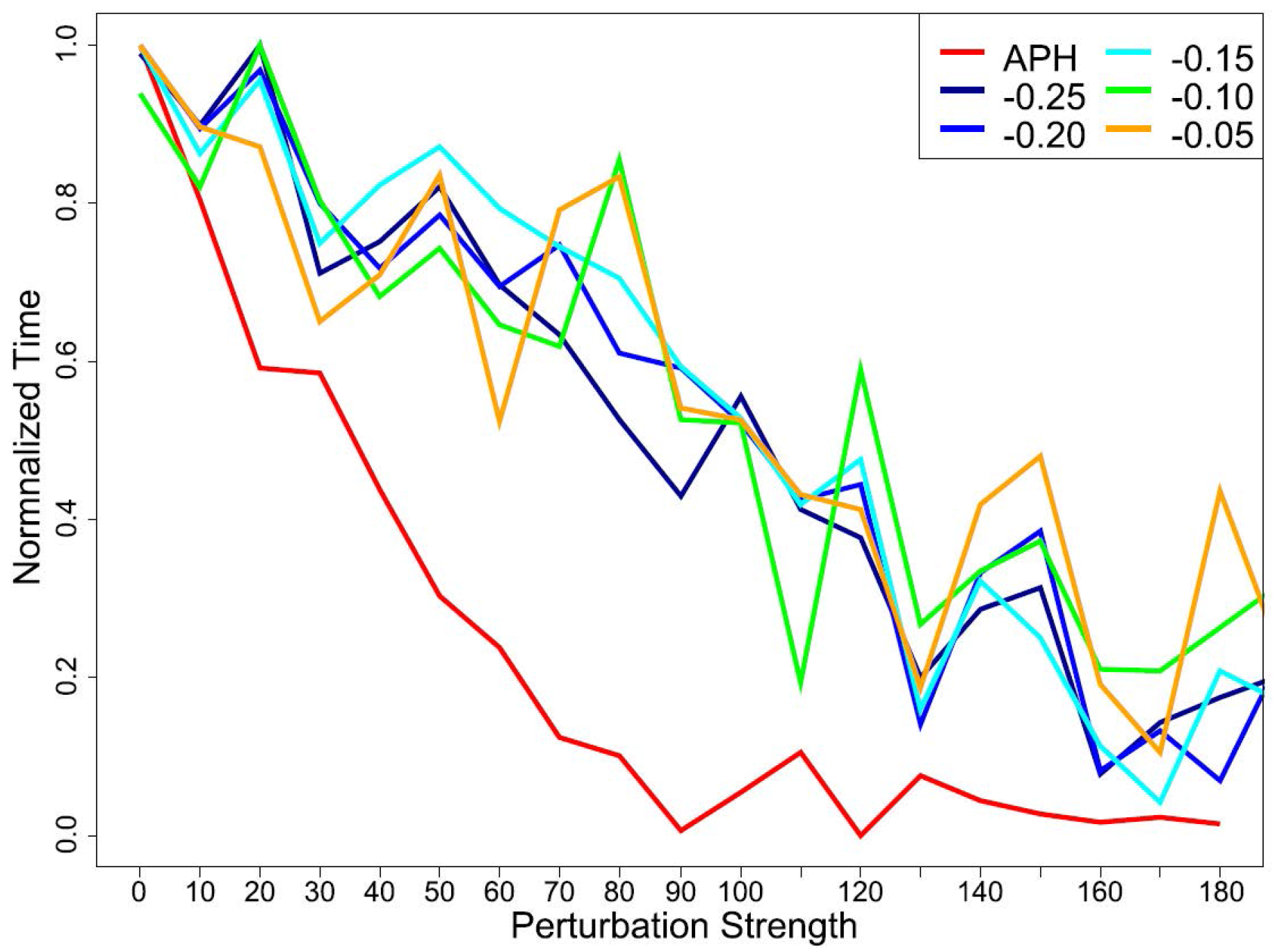
Despite the simplicity of this model it is still able to capture the dynamics of the APH based navigation. In
Figure 4 we compare the APH simulations with the perturbed Markov model in a 9 × 9 grid for different perturbation strengths. The times have been normalized between 0 and 1 to make both analyses comparable. Each
x value corresponds to the number of sources in the upper part of the grid (starting from the left top corner) for the Markovian models. For the APH simulation, each
x step corresponds to an increment of the APH persistence in 10 units. Each data point is the mean of the time arrivals obtained from 1000 simulations, each run consisting on 3000 step transitions in the lattice. The arrival times are computed by filtering the target states from the Markov chain generated with the transition matrix of Equation (
1).
From
Figure 4 it is noticed that at least statistically the APH effect can be qualitatively reproduced by means of perturbed Markov model. On the other hand, our current model is unable to produce a better agreement since ranging over different
values does not improve the fit. In a future work we will elaborate more on the model by allowing the transition matrix to carry a non-homogeneous term to better fit the APH dynamics.
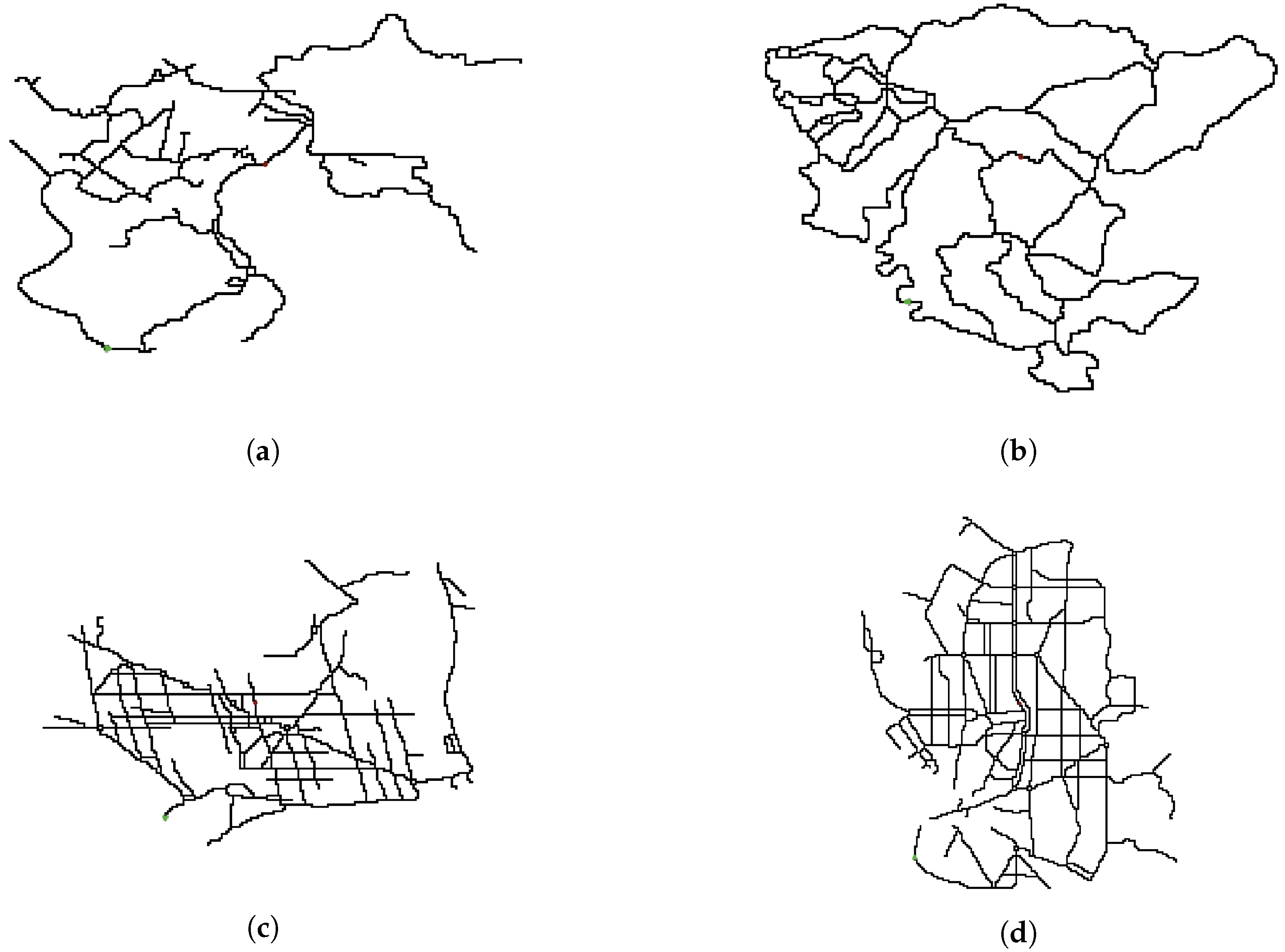
2.5. Experiments with Urban Topologies
In the last phase, we used real EV maps from the four Spanish cities commented above (see
Figure 5).
The reason for choosing these four cities is because they have a very different morphology. As stressed, every topology is parametrized by its spatial complexity R. The resulting complexities for Gijón, Castellón, Barcelona and Madrid are , , and respectively.
As in the synthetic grid experiment, the positions of the target and start are the closest possible to the center of the map and the southwest corner.
The simulation was carried out by using the same parameters of the synthetic map. For each topology—now with size—, we ran a parameter sweep with and . As before, each parameter combination was repeated 500 times.
3. Results and Discussion
In this work we proposed an algorithm to optimise the arrival times to a target with unknown location for different topologies. The experiment was repeated 500 times for the simulations and 15 times for real experiments in order to derive statistical measures. Then, for each anti-pheromone value
, we average the arrival times. Also, a scale factor was applied
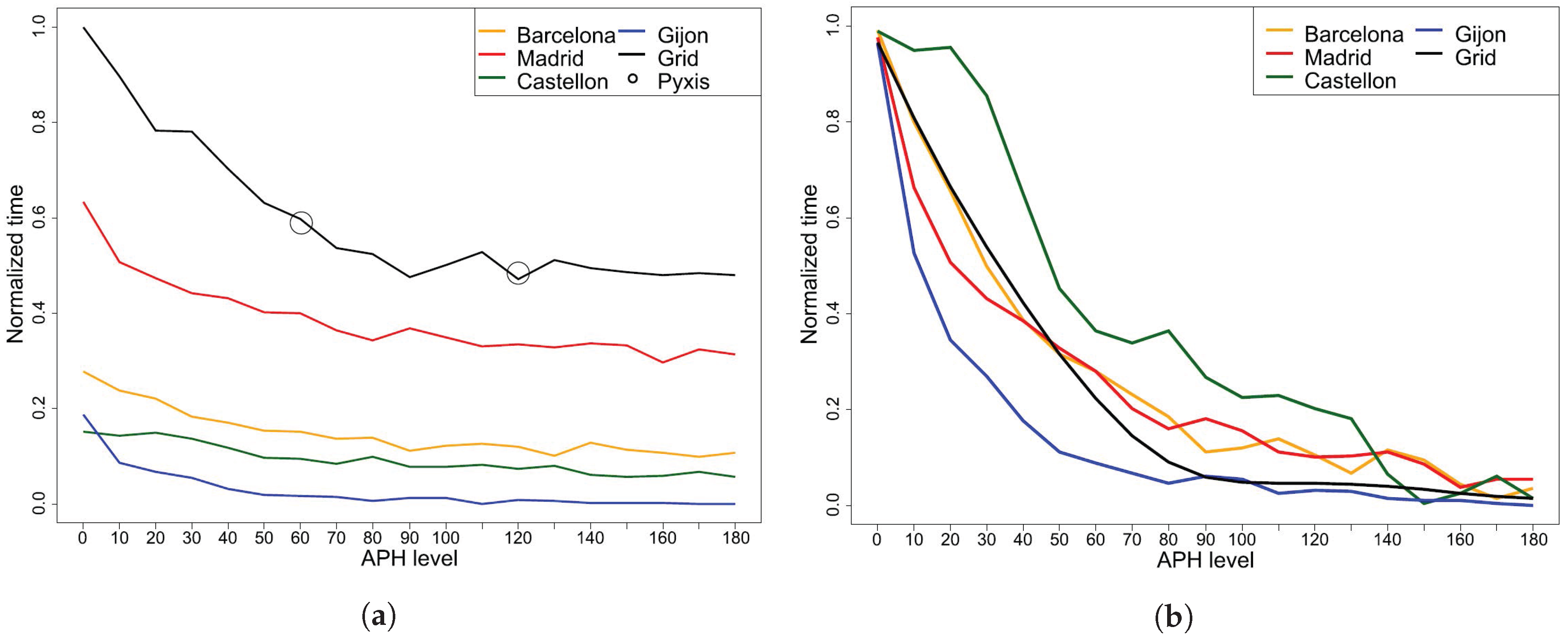
to match the different dimensions of the maps. In
Figure 6 we show the averaged times for different values of
. Here we normalized the values with the maximum and minimum arrival times for all the topologies. The black line represents the results of the numerical simulation on the grid. The two circles represent the two experiments carried out with the Pyxis robot. Finally, the color lines correspond to the cities of: Gijón, Castellón, Barcelona and Madrid. In
Figure 6b the plots have been normalized with the maximum and minimum times from each topology.
It is noticed that the general trend is that arrival times decrease as anti-pheromone evaporation increases. After the transient behavior there is a point where the times stabilize. Approximately at . The existence of an asymptotic value of allows to derive relevant bounds for the amount of information that an EV will need to optimize its exploration.
We validated the simulation with an experiment using a robot prototype. The two experiments reproduce the pattern obtained in the simulation. Hence, we can conclude that the APH algorithm for real electric vehicles performs consistently with the simulated environment that we have established.
Since time is scaled according to the map area, we can compare the times by their complexities. We notice that, as expected, increasing the map complexity increases arrival times too. The maps of Gijón (
), Castellón (
) and Barcelona (
) have a similar complexity and hence their arrival times are comparable (
Figure 6). On the other hand, the Madrid map has a larger complexity
and the arrival times are larger than those corresponding to the former cities. Finally, the arrival times obtained from the synthetic map (
) are the largest, since in this case
R is approximately three times larger than the averaged spatial complexity of the cities.
The proposed stochastic model allows to explore the local rules producing the macro-behaviour obtained with the APH algorithm. In particular we notice that it is possible to have a deterministic behaviour at large time scale despite the fact that local rules are probabilistic. As stresses, in a future work we will improve our Markovian model with a non-homogeneous component to better reproduce the observed pattern (a time-dependent component).
4. Conclusions
Energy consumption is a major concern for effective electric vehicle deployment in smart cities. In the case that an EV runs out of battery, it must be towed to the closest charging station. Therefore avoiding unnecessary cycles in an EV routing can make a substantial difference for the whole SC performance. This is particularly helpful if the charging station location is not known beforehand.
To solve this problem we have adapted a classical anti-pheromone ant foraging algorithm to the problem of finding a target with different topologies. We have validated our approach with both numerical simulations and real laboratory tests.
Firstly, we simulated the algorithm on a grid and then we validated the observed behavior in a real environment. In both cases the EV arrival times increase with the anti-pheromone evaporation times.
To gain insight into the underlying dynamics of the process we proposed a Markovian which is able to capture the main pattern observed. The number of repelling sources can be understood as a proxy of the APH level. On the other hand, the strength of the local perturbation of the transition probabilities seems to be irrelevant for the arrival time reduction. However, in a future work we will explore the possibilities of this model by considering non-homogeneous terms.
Lastly, we analysed the case of four Spanish cities; Gijón, Castellón, Barcelona and Madrid. The numerical simulations allowed us to conclude that the behavior in this case is similar to that obtained in the previous experiments and qualitatively comparable to the results of the theoretical model.
The approach presented in this work can be valuable to solve the problem of finding charging stations with unknown location. As a first step we considered a hypothetical situation in which there is only one charging point. However, in a future work we will tackle the problem of various charging stations distributed over the map. This will render the current approach into a more realistic setting.
Another strategy to improve this algorithm is to enable swarm behavior by Using a swarm of electric vehicles. In this case regardless of the number of charging points the exploration elapsed times could be significantly reduced. In a future work we will also explore this aggregated behaviour.
Finally, the modeling of potential conflicts at intersections is a logical step in this development. In a future project we will consider this problem through the same multi-agent approach that we have used in this work.


 ,
, 


