Article

Non-Convex Economic Dispatch of a Virtual Power Plant via a Distributed Randomized Gradient-Free Algorithm

1
College of Automation, Nanjing University of Posts and Telecommunications, Nanjing 210023, China
2
College of Energy and Electrical Engineering, Hohai University, Nanjing 211100, China
*
Author to whom correspondence should be addressed.
Energies 2017, 10(7), 1051; https://doi.org/10.3390/en10071051
Submission received: 26 June 2017 / Revised: 18 July 2017 / Accepted: 19 July 2017 / Published: 21 July 2017
(This article belongs to the Section F: Electrical Engineering)

Abstract

:
The economic dispatch problem of a virtual power plant (VPP) is becoming non-convex for distributed generators’ characteristics of valve-point loading effects, prohibited operating zones, and multiple fuel options. In this paper, the economic dispatch model of VPP is established and then solved by a distributed randomized gradient-free algorithm. To deal with the non-smooth objective function, its Gauss approximation is used to construct distributed randomized gradient-free oracles in optimization iterations. A projection operator is also introduced to solve the discontinuous variable space problem. An example simulation is implemented on a modified IEEE-34 bus test system, and the results demonstrate the effectiveness and applicability of the proposed algorithm.

1. Introduction

Distributed energy resources (DERs) include distributed generators (DGs), renewable energies (REs), and energy storage systems (ESs) [1]. Optimizing the output of DERs can greatly improve the efficiency of their energy utilization. The centralized dispatch methods adopt lambda iterative algorithms [2] and interior point lambda iterative algorithms [3], both of which need the objective functions to be smooth and derivable. Actually, the cost functions of DGs are non-convex because of their features of valve-point loading effects, prohibited operating zones, and multiple fuel options [4]. The charging and discharging of ESs also aggravates the complexity of economic dispatch problems [5]. Based on advanced management concepts and software technologies, the virtual power plant (VPP) [6,7] has been developed to be a new DERs management tool. Additionally, it is necessary to solve the non-convex economic dispatch of VPPs in order to realize the optimal scheduling of DERs. Intelligent optimization algorithms can solve non-convex optimization problems effectively, including the genetic algorithm (GA) [8], particle swarm optimization (PSO) [9], and differential evolution [10,11]. However, these algorithms rely on the dispatch center or controller to collect and process DERs’ information, which may lead to a higher communication cost; they also need a centralized communication structure with high bandwidth, which has poor system reliability and is more vulnerable to a single point of failure [12].
At present, the optimization decision process of VPPs is changing from centralized ways to distributed ones [13]. According to the local communication mechanism, the operation information of the DERs is collected through communication lines built among DER units and their adjacent units, and then the real-time scheduling process can be carried out. The distributed consensus algorithm employed in the distributed scheduling of [14] can greatly reduce communication costs and communication delays. Compared with centralized solutions, the distributed gradient algorithm in [15] can not only obtain comparable optimums but also respond in a timely manner when the operation conditions of the system change. To solve the problem of the objective function of ESs being not smooth, the sub-gradient is calculated as an alternative of the gradient [16,17]. The economic dispatch of a VPP is a non-convex optimization problem for the consideration of valve-point loading effects, prohibited operating zones, and multiple fuel options. The algorithms mentioned in [14,15,16,17] cannot be applied to the non-convex optimization problem because it is difficult to estimate the gradient or sub-gradient. The distributed auction-based algorithm designed in [12] can realize the optimal power output by sharing units’ bidding and then determining the auction results in the process of consensus. However, it introduces too many intermediate variables, which will make the iteration format more complex.
This paper adopts a distributed randomized gradient free algorithm (DRGF) [18] to solve a VPP's non-convex economic dispatch problem considering DGs’ valve-point loading effects, prohibited operating zones, and multiple fuel options. The algorithm is established on a distributed communication structure that has a higher operation reliability and lower communication cost [12]. In addition, the DRGF approach calculates randomized gradient-free oracles, instead of gradients or sub-gradients, to implement the distributed optimization, which makes the iteration formula simple and easily solved. The modified IEEE-34 bus system is employed to verify the effectiveness of the proposed method. The simulation results show that the DRGF algorithm can formulate an economical scheme for a VPP’s non-convex economic dispatch.
This paper is organized as follows. In Section 2, a VPP’s non-convex economic dispatch with constraints of valve-point loading effects, prohibited operating zones, and multiple fuel options is discussed. Section 3 introduces the DRGF algorithm, and the simulation results presented in Section 4 show its effectiveness. Finally, the paper is summarized in Section 5.

2. VPPs’ Non-Convex Economic Dispatch

2.1. The Operation Models of the DER’s Units

In traditional economic dispatch, the cost function of a DG is a standard quadratic function [19]. If valve-point loading effects, simulated by sinusoidal terms, and multiple fuel options are taken into account, the cost function can be described as [4,12]:
C ( P i ) = { a i 1 P i 2 + b i 1 P i + c i 1 + | d i 1 sin ( e i 1 P i e i 1 P i min ) | , P i min P i P 1 i       i = 1 , , n g . a i q P i 2 + b i q P i + c i q + | d i q sin ( e i q P i e i q P i min ) | , P ( q 1 ) , i P i P i max ,
where ng is the total number of DGs and the power output of DGi is Pi, yielding to the upper limit P i max and lower limit P i min . When Pi exceeds the value of P(q-1),i, unit i chooses the fuel q and its cost function C(Pi) uses coefficients of a i q , b i q , c i q , d i q , e i q .
Because the power output is usually concentrated in some areas, the operational efficiency can be greatly promoted by prohibiting units from running in low productivity areas. The power output constraints considering DGs’ prohibited operating zones can be expressed as [4,12]:
{ P i min P i L m i , m i = 1 U ( m 1 ) i P i L m i , m i = 2 , , M i . U m i P i P i max , m i = M i ,
where unit i has Mi prohibited operating zones, the mith of which subjects to the upper boundary Umi and lower boundary Lmi.
ESs can work in charging or discharging modes, and their cost functions and operation constraints are as follows [20,21]:
C ( P e i ) = 0.5 E i | P e i |   ,   e i = 1 , , n e . ,
P c h max P e i P d c h max ,
{ S u p < S O C S max , d c h S d o w n S O C S u p , d c h   o r   c h   S min S O C < S d o w n , c h ,
where ne is the total number of ESs, and the power output of ESi is Pei. C (Pei) represents the charging (ch)/discharging (dch) cost, and Ei is the charging/discharging efficiency. The maximum charging and discharging power of ESi is P c h max , P d c h max . Additionally, the minimum of both is 0. For the value of the state-of-charge (SOC), Smax, Smin, Sup, Sdown are the maximum, minimum, upper, and lower values, respectively [20].
Compared with operating at maximum power, REs will be more flexible in a schedulable mode. However, this will also cause some profit losses, that is, the schedulable cost C (Pri) [21]:
C ( P r i ) = ρ V   ( o r   ρ W )   [ P r i max P r i ]   ,   r i = 1 , , n r .
s . t .   0 P r i P r i max
where nr is the total number of REs, and the power output of REi is Pri. The ρ V (photovoltaic systems) and ρ W (wind turbine) are the grid-connected prices, including electricity prices and generation compensations. The maximum available power of REi is P r i max , and it can be either the maximum photovoltaic system tracking power PV [22] or the maximum wind power PW [23]:
P V = P V max G C G C max [ 1 + K ( T c T r ) ] ,
P W = { 0 v < v c i , v v c o v v c i v r v c i P r v c i < v < v r P r v r v v c o ,
where PVmax represents the maximum output under standard test conditions. GC means the actual light intensity; GCmax is the reference intensity under standard test conditions. The conversion coefficient of temperature to power is depicted by K. Tc and Tr are the environment temperature and the reference temperature under standard test conditions, respectively. Pr is the rated power output of the wind generators (WGs). v, vci, vco, and vr are the wind speeds, cut-in wind speeds, cut-out wind speeds, and the rated wind speeds, respectively.

2.2. Dispatch Objectives and Constraints

According to the operation mode of a VPP, the economic dispatch objective function and the system constraints can be defined as [16,21]:
max F V P P = ρ d P D + ρ s P S C V P P ,
C V P P = i = 1 n g C ( P i ) + i = 1 n e C ( P e i ) + i = 1 n r C ( P r i ) ,
i = 1 n g P i + i = 1 n e P e i + i = 1 n r P r i = P D + P S ,
P V P P max P D γ 1 P D + γ 2 P V + γ 3 P W ,
where FVPP denotes the total income of the VPP, and CVPP represents its total generation cost. The maximum generation capacity of the VPP is P V P P max , that is, the sum of the maximum power output of each DER unit. The total load demand is PD and PS is the interface power at the point of common coupling (PCC). If PS is negative, the power will flow from the VPP into the main grid. ρd is the bidding of the VPP and ρS is the electricity price of the main grid. γ1, γ2, and γ3 are the reserved capacity coefficients of the load demand, photovoltaic systems, and wind turbines, respectively.

3. Distributed Randomized Gradient-Free (DRGF) Algorithm

The DERs’ power output vector P = [ P 1 , P 2 , P n g , P e 1 , P e 2 , P n e , P r 1 , P r 2 , P n r ] T can be denoted as a variable vector x = [ x 1 , x 2 , x n ] T , and there exists n = n g + n e + n r . Accordingly, the upper and lower bounds of the variables are represented by x i max , x i min . Thus, the active power balance constraint of the original VPP economic dispatch problem can be denoted as:
P S = i = 1 n x i P D ,
Substituting formula (14) into formula (10), one can obtain:
max F V P P = ( ρ d ρ s ) P D i = 1 n [ C ( x i ) ρ s x i ] ,
It can be seen that the FVPP is only dependent on variables xi when the values of ρd, ρS, and PD are constant. If we set f i ( x i ) = C ( x i ) ρ s x i , the original objective function can be equivalent to a minimization problem:
min x X f ( x ) = i = 1 n f i ( x i ) ,
where f(x) denotes the objective function, and X is the feasible space of x, that is, xX may represent the power output constraints of DERs.
Based on a distributed optimization framework, the DERs can collect neighboring units’ information and the information at the PCC, and then this information will be calculated by weighted mean values [14,18]
x i ¯ [ k ] = j = 1 n W i j [ k ] x j [ k ] + ε i P S ,
where εi is the power regulation factor, and x i ¯ is the weighted mean value of xi. Unit j is connected to unit i with the communication weight Wij [k], and its calculation format is shown in [12].
This paper employs a DRGF algorithm [18] to solve the problems of a discontinuous solution space and the non-convex objective function. Although the objective function of a VPP is not smooth, it is Lipschitz continuous in the variable space [24], and its smooth form can be written as:
min x X f μ ( x ) = i = 1 n f i μ i ( x i ) ,
where μi is the smoothing coefficient of the objective function, and f i μ i ( x i ) is its smooth form, calculated by:
f i μ i ( x i ) = 1 γ X f i ( x i + μ i τ i ) e 0.5 τ 2 d τ i ,
where the conversion coefficient denotes as γ = ( 2 π ) n , and the random sequence τi meets the Gaussian distribution. The theory of Gauss approximation is shown in the Appendix A.
Now, distributed randomized gradient-free oracles can be constructed to implement the optimal iteration:
g μ i ( x i [ k ] ) = f i μ i ( x i [ k ] + μ i τ i [ k ] ) f i μ i ( x i [ k ] ) μ i τ i [ k ] ,
where g μ i ( x i [ k ] ) represents the distributed randomized gradient-free oracle of xi at the kth iteration.
By the above steps, the iterative form of the optimization variables can be derived as:
x i [ k + 1 ] = P X [ x i ¯ [ k ] α [ k ] g μ i ( x i [ k ] ) ] ,
where the projection operator PX is defined as in [25]. The iteration step-size satisfies the following conditions:
α [ k ] > 0 , k = 0 α [ k ] = , k = 0 ( α [ k ] ) 2 < ,
The implementation process of a VPP’s non-convex economic dispatch via the DRGF algorithm is shown in Figure 1, and the specific procedures are as follows:
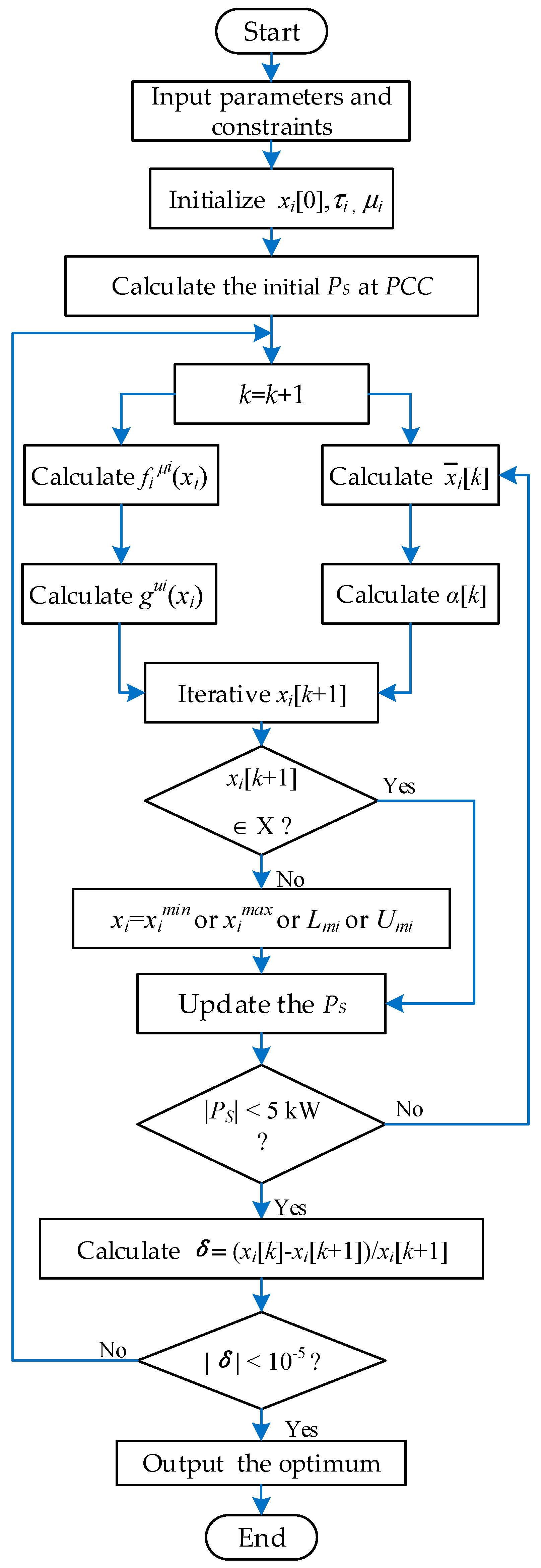
  • The input data includes the coefficients of cost functions, various limits of the DERs’ power output, the total load demand, etc. The maximum available power output of the REs is calculated by formula (8) and (9).
  • The optimization variable xi [0] is initialized according to references [8,10,15]. Then, set up the smoothing coefficient of the objective function and generate the random sequence.
  • According to formula (14), calculate the initial PS at PCC.
  • Correct the iteration step by k = k + 1, where the initial number of iteration steps is k = 1.
  • According to formula (17), calculate the weighted mean values; and according to formula (19), calculate the Gauss approximation. When DGs have multiple fuel options, as shown in equation (2), select the cost function curves on the basis of the DG’s actual power output.
  • According to formula (20), calculate distributed randomized gradient-free oracles; according to formula (22), calculate the current iteration step by α [ k ] = 1 / k + 1 .
  • According to formula (21), implement the optimal iteration of the power output variables.
  • Determine whether the current variables are within the available space. If they satisfy, proceed to the next step; otherwise, the variables take the upper ( x i [ k + 1 ] x i max ) or lower ( x i [ k + 1 ] x i min ) limits of the constraints. When variable xi falls into prohibited zone mi during the decreasing process, such as xi [k] > xi [k + 1], its value will be set at the upper boundary Umi. Additionally, when xi falls into prohibited zone mi during the increasing process, such as xi [k] < xi [k + 1], the value will be set at the lower boundary Lm.
  • According to formula (14), update the initial PS at PCC.
  • Determine whether the current power imbalance satisfies the allowable value. If it satisfies, proceed to the next step; otherwise, return to step (5) to recalculate the weighted mean values.
  • Calculate the iteration error.
  • Determine whether the iteration error satisfies the allowable value. If it satisfies, proceed to the next step; otherwise, return to step (4) for the next iteration.
  • Output the optimal solution vector.

4. Numerical Examples

Based on a modified IEEE 34 bus system, a VPP system is built to verify the effectiveness of the proposed algorithm. It mainly investigates DGs’ valve-point loading effects, prohibited operating zones, and multiple fuel options. The reference [18] shows that the convergence coefficient has little effect on the convergence of the algorithm, so the smoothing coefficient of the cost function is set to 0.0005 in this example. The communication topology is shown in Figure 2. The operation parameters are listed in Table 1 and Table 2. The total load demand is 650 kW, and the initial power outputs of the DGs, REs, and ESs are 75, 75, and 0 kW, respectively. For solving non-convex economic dispatch problems, a PSO solution used in [9] has achieved the lowest cost among numerous centralized algorithms. As contrast, we will also adopt the PSO [9] (one of the centralized dispatch method) to deal with the VPP’s economic dispatch model. Table 3 provides the optimization results when one of the centralized dispatch method (PSO) is adopted, and Table 4 shows the VPP’s average profits made by PSO and DRGF. This section sets up three simulation scenarios as follows: (A) the VPP’s distributed economic dispatch with valve-point loading effects; (B) the VPP’s distributed economic dispatch with prohibited operating zones; (C) the VPP’s distributed economic dispatch with multiple fuel options.

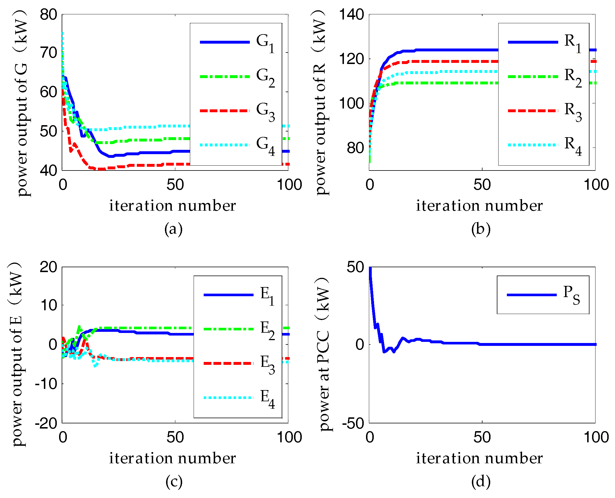
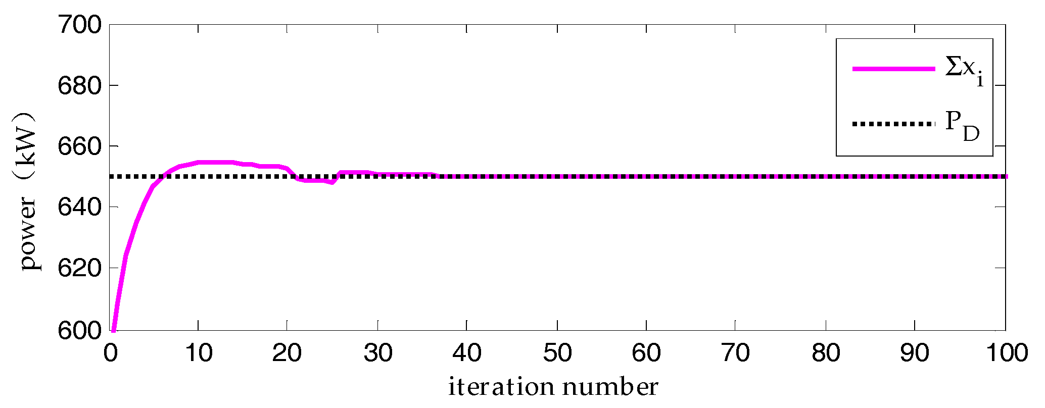
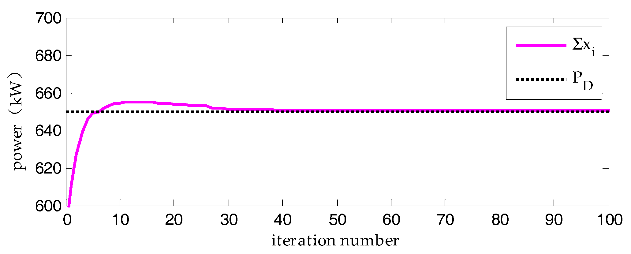
4.1. Scenario A: The VPP’s Distributed Economic Dispatch with Valve-Point Loading Effects

The characteristic of valve-point loading effects makes the DGs’ cost function have many non-differentiable points. The operation coefficients of DGs are shown in Table 1 and Table 2. Figure 3 and Figure 4 provide the optimal scheduling process of this scenario. It can be seen that the DGs’ power output will have a great fluctuation during the initial stage of optimization, and then the ESs will change their power output to reduce the impact of valve-point loading effects on the system’s active power balance. In addition, the VPP also exchanges power with the main grid through the PCC to stabilize the supply-demand balance. After a certain number of iterations, the DERs’ optimization curves tend to be stable, and the DRGF algorithm finally achieves the same results as centralized algorithms (shown in Table 3 and Table 4). However, if considering the communication cost and operability, the distributed dispatch will be more economical and practical.

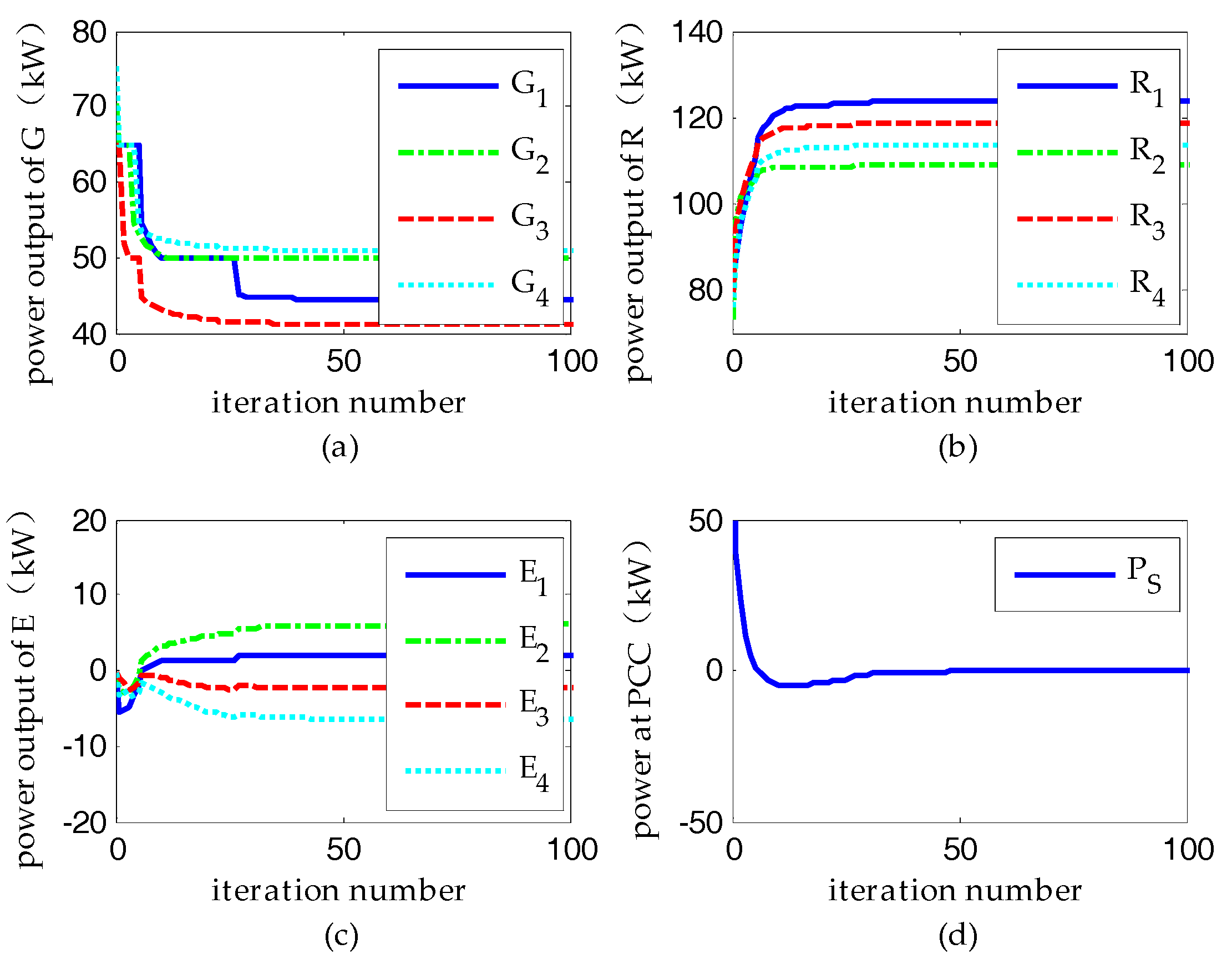
4.2. Scenario B: The VPP’s Distributed Economic Dispatch with Prohibited Operating Zones

The DGs’ power output is discontinuous for some prohibited operating zones. Figure 5 and Figure 6 show the simulation results under this scenario. In Figure 5a, the platforms in the curve indicate the situation where DGs fall into prohibited operating zones. When DGs jump out of these areas, they will resume normal operation. ESs can flexibly charge and discharge, greatly reducing the impact of prohibited operating zones on the active power balance. As can be seen from Table 3, the DRGF algorithm can get the same results as the centralized algorithms, which demonstrates that the DRGF algorithm can effectively deal with DGs’ prohibited operating zones.

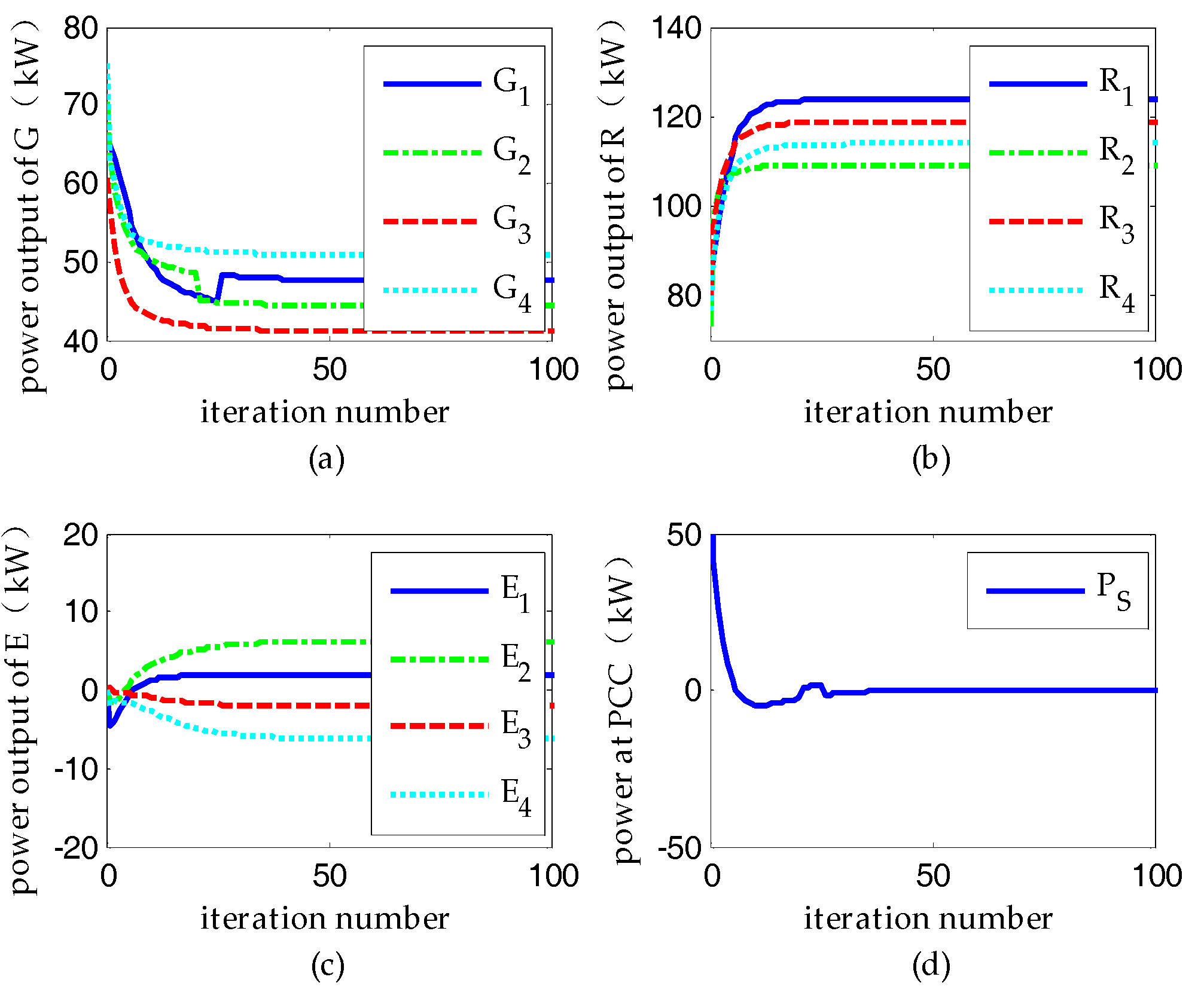
4.3. Scenario C: the VPP’s Distributed Economic Dispatch with Multiple Fuel Options

According to actual power output, DGs will choose the most economical fuel selection with different cost coefficients, leading to some non-differentiable points. Figure 7 and Figure 8 provide this scenario’s simulation results. In Figure 7a and Table 1, when the power output is within 40–55 kW, DGs select the No. 1 fuel; if the power output is within 55–80 kW, DGs will select the No. 2 fuel. Then, the allocation of DERs should be re-optimized. The VPP’s total power output may have a large fluctuation when the fuel changes, and the system will recover the active power balance quickly by absorbing some power from the main grid. The distributed dispatch can get the same result as the centralized one, which shows the DRGF algorithm’s effectiveness in solving DGs’ multiple fuel options.

5. Summary

A technology of a VPP is adopted to manage DERs by modeling its non-convex economic dispatch considering DGs’ characteristics of valve-point loading effects, prohibited operating zones, and multiple fuel options. A DRGF algorithm is introduced to solve this nonlinear and non-differentiable optimization problem. The objective function is converted to its Gauss approximation, and then used to construct distributed randomized gradient-free oracles instead of gradients or sub-gradients. A projection operator is also employed to deal with the discontinuous variable space. Three typical simulation scenarios are implemented on a modified IEEE 34 bus system. The results indicate that the proposed DRGF algorithm can effectively cope with a VPP’s non-convex economic dispatch, and shows a good applicability.

Acknowledgment

This study is supported by the Major State Basic Research Development Program of China (Grant No. 2016YFB0901100) and the National Science Foundation of China (Grant No. 51577051).

Author Contributions

All of the authors contributed to this work. Jun Xie provided critical guidance to this research and checked the overall logic of this work. Chi Cao designed the study, developed the mathematical model, and performed the analysis and simulations.

Conflicts of Interest

The authors declare no conflict of interest.

Appendix A

According to [24] (theorem 1 and 4, Formula (11) and (22)), the following lemma is introduced to provide some important properties of the function f i μ i ( x i ) and the random gradient-free oracle g μ i ( x i [ k ] ) .
Lemma A1. 
For each i, there has:
(a) 
f i μ i ( x i ) is convex and differentiable, and it satisfies:
f i ( x i ) f i μ i ( x i ) f i ( x i ) + n μ i G 0 ( f i ) ,
(b) 
The gradient f i μ i ( x i ) satisfies:
Ε [ g μ i ( x i [ k ] ) ] = f i μ i ( x i ) ,
(c) 
The random gradient-free oracle satisfies:
Ε [ g μ i ( x i [ k ] ) 2 ] ( n + 4 ) 2 G 0 ( f i ) 2 ,
where G0(fi) is Lipschitz constant; E[x] denotes the expected value of a random variable x. The further principle description and proof can be found in [18,24].

References

  1. Safdarian, A.; Firuzabad, M.F.; Lehtonen, M.; Aminifar, F. Optimal electricity procurement in smart grids with autonomous distributed energy resources. IEEE Trans. Smart Grid 2015, 6, 2975–2984. [Google Scholar] [CrossRef]
  2. Lin, C.E.; Viviani, G.L. Hierarchical economic dispatch for piecewise quadratic cost functions. IEEE Trans. Power Appl. Syst. 1984, 103, 1170–1175. [Google Scholar] [CrossRef]
  3. Lin, W.M.; Chen, S.J. Bid-based dynamic economic dispatch with an efficient interior point algorithm. Int. J. Electr. Power Energy Syst. 2002, 24, 51–57. [Google Scholar] [CrossRef]
  4. Pattanaik, J.K.; Basu, M.; Dash, D.P. Review on application and comparison of metaheuristic techniques to multi-area economic dispatch problem. Prot. Control Mod. Power Syst. 2017, 2, 2–11. [Google Scholar] [CrossRef]
  5. Teng, J.H.; Luan, S.W.; Lee, D.J.; Huang, Y.Q. Optimal charging/discharging scheduling of battery storage systems for distribution systems interconnected with sizeable PV generation systems. IEEE Trans. Power Syst. 2013, 28, 1425–1433. [Google Scholar] [CrossRef]
  6. Pudjianto, D.; Ramsay, C.; Strbac, G. Virtual power plant and system integration of distributed energy resources. IET Renew. Power Gener. 2007, 1, 10–16. [Google Scholar] [CrossRef]
  7. Ai, Q.; Fan, S.L.; Piao, L.J. Optimal scheduling strategy for virtual power plants based on credibility theory. Prot. Control Mod. Power Syst. 2016, 1, 1–8. [Google Scholar] [CrossRef]
  8. Chiang, C. L. Improved genetic algorithm for power economic dispatch of units with valve-point effects and multiple fuels. IEEE Trans. Power Syst. 2005, 20, 1690–1699. [Google Scholar] [CrossRef]
  9. Selvakumar, A.I.; Thanushkodi, K. A new particle swarm optimization solution to nonconvex economic dispatch problems. IEEE Trans. Power Syst. 2007, 22, 42–51. [Google Scholar] [CrossRef]
  10. Bhattacharya, A.; Chattopadhyay, P.K. Hybrid differential evolution with biogeography based optimization for solution of economic load dispatch. IEEE Trans. Power Syst. 2010, 25, 1955–1964. [Google Scholar] [CrossRef]
  11. Pattanaik, J.K.; Basu, M.; Dash, D.P. Opposition-based differential evolution for hydrothermal power system. Prot. Control Mod. Power Syst. 2017, 1, 1–17. [Google Scholar] [CrossRef]
  12. Binetti, G.; Davoudi, A.; Naso, D.; Turchiano, B.; Lewis, F.L. A distributed auction-based algorithm for the non-convex economic dispatch problem. IEEE Trans. Ind. Inf. 2014, 10, 1124–1132. [Google Scholar] [CrossRef]
  13. Yang, Q.; Barria, J.A.; Green, T.C. Communication infrastructures for distributed control of power distribution networks. IEEE Trans. Ind. Inf. 2011, 7, 316–327. [Google Scholar] [CrossRef]
  14. Rahbari-Asr, N.; Unnati, O.; Zhang, Z.; Chow, M.Y. Incremental welfare consensus algorithm for cooperative distributed generation/demand response in smart grid. IEEE Trans. Smart Grid 2014, 5, 2836–2845. [Google Scholar] [CrossRef]
  15. Zhang, W.; Liu, W.; Wang, X. Online optimal generation control based on constrained distributed gradient algorithm. IEEE Trans. Power Syst. 2015, 30, 35–45. [Google Scholar] [CrossRef]
  16. Yang, H.M.; Yi, D.X.; Zhao, J.H.; Dong, Z.Y. Distributed optimal dispatch of virtual power plant via limited communication. IEEE Trans. Power Syst. 2013, 28, 3511–3512. [Google Scholar] [CrossRef]
  17. Cao, C.; Xie, J.; Yue, D.; Huang, C.X.; Wang, J.X.; Xu, S.Y.; Chen, X.Y. Distributed Economic Dispatch of Virtual Power Plant under Non-ideal Communication Network. Energies 2017, 10, 235. [Google Scholar] [CrossRef]
  18. Yuan, D.M.; Ho Daniel, W.C. Randomized gradient-free method for multi agent optimization over time-varying networks. IEEE Trans. Neural Learn. Syst. 2015, 26, 1342–1347. [Google Scholar] [CrossRef] [PubMed]
  19. Yang, Z.Q.; Xiang, J.; Li, Y.J. Distributed consensus based supply–demand balance algorithm for economic dispatch problem in a smart grid with switching graph. IEEE Trans. Ind. Electron. 2017, 64, 1600–1610. [Google Scholar] [CrossRef]
  20. Lu, X.N.; Sun, K.; Guerrero, J.M.; Vasquez, J.C.; Huang, L.P. State-of-charge balance using adaptive droop control for distributed energy storage systems in DC micro-grid applications. IEEE Trans. Ind. Electron. 2014, 61, 2804–2815. [Google Scholar] [CrossRef]
  21. Wang, Y.; Ai, X.; Tan, Z.F.; Yan, L.; Liu, S.T. Interactive Dispatch Modes and Bidding Strategy of Multiple Virtual Power Plants Based on Demand Response and Game Theory. IEEE Trans. Smart Grid 2016, 7, 510–519. [Google Scholar] [CrossRef]
  22. Gavanidou, E.S.; Bakirtzis, A.G. Design of a stand alone system with renewable energy sources using trade off methods. IEEE Trans. Energy Convers. 1992, 7, 42–48. [Google Scholar] [CrossRef]
  23. John, H.; David, C.Y.; Kalu, B. An economic dispatch model incorporating wind Power. IEEE Trans. Energy Convers. 2008, 23, 603–611. [Google Scholar]
  24. Nesterov, Y.; Spokoiny, V. Random gradient-free minimization of convex functions. Found. Comput. Math. 2017, 17, 527–566. [Google Scholar] [CrossRef]
  25. Nedic, A.; Ozdaglar, A.; Parrilo, P.A. Constrained consensus and optimization in multi-agent networks. IEEE Trans. Autom. Control 2010, 55, 922–938. [Google Scholar] [CrossRef]
Figure 1. The flowchart for a virtual power plant’s (VPP’s) non-convex economic dispatch via the distributed randomized gradient free algorithm (DRGF) algorithm.
Energies 10 01051 g001
Figure 2. The communication topology based on a modified IEEE 34 bus system.
Energies 10 01051 g002
Figure 3. The optimized scheduling scheme of scenario A: (a) Optimization results of distributed generators (DGs); (b) Optimization result of renewable energies (REs); (c) Optimization results of energy storage systems (ESs); (d) The power PS at the point of common coupling (PCC).
Energies 10 01051 g003
Figure 4. The active power balance of scenario A.
Energies 10 01051 g004
Figure 5. The optimized scheduling scheme of scenario B: (a) Optimization results of DGs; (b) Optimization result of REs; (c) Optimization results of ESs; (d) The power PS at PCC.
Energies 10 01051 g005
Figure 6. The active power balance of scenario B.
Energies 10 01051 g006
Figure 7. The optimized scheduling scheme of scenario C: (a) Optimization results of DGs; (b) Optimization result of REs; (c) Optimization results of ESs; (d) The power PS at PCC.
Energies 10 01051 g007
Figure 8. The active power balance of scenario C.
Energies 10 01051 g008
Table 1. Coefficients of the distributed generators’ (DGs’) production cost. DER, Distributed Energy Resources.
DERs UnitsFuel Type a i q P i 2 + b i q P i + c i q + | d i q sin ( e i q P i e i q P i min ) | ($/kWh)Operation Range (kW)
aibicidiei
DG 110.075125.734996.573100.05340–55
20.057821.462996.572950.04855–80
DG 210.081421.2151002.12250.06240–55
20.058119.8931002.12180.06155–80
DG 310.085722.1881058.34360.04240–55
20.059622.0951058.34020.04155–80
DG 410.070428.026978.522890.04640–55
20.067227.684978.522750.03955–80
Table 2. The virtual power plant’s (VPP’s) other operation parameters.
Operation ParametersValues
γ1, γ2, γ30.05, 0.2, 0.15
SOC(min, down, up, max)0.05, 0.20, 0.80, 0.95
[L1, U1], [L2, U2][45, 50], [55, 65] (kW)
ρrV, ρrW, ρd, ρS0.0839, 0.0721, 0.0780, 0.0736 ($/kWh)
Ei; EC; Pmax(ch, dch)85%; 100 (kWh); 20, 20 (kW)
Pr; v, vci, vco, vr120 (kW); 12, 3.0, 25, 15 (m/s)
PVmax; GCmax, GC; K; Tr, Tc180 (kW); 1, 0.9 (kw/m2); −0.45%; 25, 18 (°C)
Table 3. Optimization results under one of the centralized dispatch method (PSO).
Distributed Energy Resources(DERs) UnitsThe Optimization Results (kW)
Scenarios AScenarios BScenarios C
Distributed Generator (DG) 144.636444.412847.6625
Distributed Generator (DG) 247.885050.000044.4135
Distributed Generator (DG) 341.385541.163741.1637
Distributed Generator (DG) 451.134550.913350.9136
Renewable Energy (RE) 1123.7492123.5162123.7500
Renewable Energy (RE) 2109.0612108.8276109.0614
Renewable Energy (RE) 3118.8540118.6203118.8541
Renewable Energy (RE) 4113.9585113.7249113.9587
Energy Storage (ES) 12.67561.84962.0834
Energy Storage (ES) 24.25156.01706.2511
Energy Storage (ES) 3−3.4227−2.3173−2.0838
Energy Storage (ES) 4−4.4134−6.4850−6.2517
Table 4. The VPP’s average profits obtained by two dispatch strategies (PSO and DRGF).
AlgorithmThe PSO [8]The DRGF
Scenarios a0.0642 ($/kWh)0.0642 ($/kWh)
Scenarios b0.0645 ($/kWh)0.0645 ($/kWh)
Scenarios c0.0649 ($/kWh)0.0649 ($/kWh)

