Energy Modelling and Automated Calibrations of Ancient Building Simulations: A Case Study of a School in the Northwest of Spain

Abstract

In the present paper, the energy performance of buildings forming a school centre in the northwest of Spain was analyzed using a transient simulation of the energy model of the school, which was developed with TRNSYS, a software of proven reliability in the field of thermal simulations. A deterministic calibration approach was applied to the initial building model to adjust the predictions to the actual performance of the school, data acquired during the temperature measurement campaign. The buildings under study were in deteriorated conditions due to poor maintenance over the years, presenting a big challenge for modelling and simulating it in a reliable way. The results showed that the proposed methodology is successful for obtaining calibrated thermal models of these types of damaged buildings, as the metrics employed to verify the final error showed a reduced normalized mean bias error (NMBE) of 2.73%. It was verified that a decrease of approximately 60% in NMBE and 17% in the coefficient of variation of the root mean square error (CV(RMSE)) was achieved due to the calibration process. Subsequent steps were performed with the aid of new software, which was developed under a European project that enabled the automated calibration of the simulations.

1. Introduction

In recent decades, energy efficiency in buildings has taken a significant role in energy savings, both at the national and European level. In fact, energy certification of buildings is currently a requirement derived from European directives [1,2] regarding the energy efficiency of buildings in which their objective is to promote energy audits to facilitate the implementation of energy-saving measures. It is known that more than 40% of the total energy consumption in the European Union (EU) is due to buildings [1]. Regarding old buildings, whose facilities have deteriorated over time, these buildings pose an especially high energy cost. Currently, approximately 35% of the EU's buildings are over 50 years old [3]. In Spain, most educational centres are considered old buildings because they were built at the beginning of the 20th century with a similar typology [4]. The school sector in Europe accounts for approximately 20% of all of the non-residential buildings [5]. These educational buildings consume an average of 13% of total energy in the USA, 4% in Spain and 10% in the UK [6]. For these reasons, it is particularly important to perform a survey of their energy situation through which it is possible to propose energy saving measures in a reliable way [7,8]. This is a subject that is gaining interest in recent years, since many authors are studying the possibility of energy savings in schools [9,10,11].

Under these circumstances, building energy performance simulation (BEPS) software programs have lately become essential tools because they provide an evaluation of the behavior of a building with a high degree of accuracy. BEPS tools, such as Energy Plus, DOE-2, TRNSYS or ESP-r, are being widely used currently by other authors [12,13], and more specifically TRNSYS [14] has been verified to achieve results with a high accuracy [15,16,17,18].

While it is true that BEPS software has the ability to provide simulations according to the actual installation, the modeller (while developing the model) has to make assumptions based on his previous experience, which sometimes causes a high degree of uncertainty [19]. This is when calibration becomes important, particularly for ancient buildings [20]. Through a calibration process, the model simulated is fine-tuned to yield predicted results that are more adjusted to the observed data that was registered from the actual system (namely, energy demand or inside air conditions, such as temperature or humidity). There are currently different calibration methodologies, and there is still no agreement on which is the most appropriate for each problem [21], although most of these calibration efforts are built upon the recommendations provided by ASHRAE Guideline 14 [22], which provides metrics and acceptable tolerances to establish whether the computer model of an entire building can be considered calibrated. This paper introduces a procedure to model, simulate and calibrate the thermal behavior of buildings so a high degree of reliability and accuracy can be obtained when validating the results of the simulation with the data obtained by monitoring the real system.

The simulating engine employed was TRNSYS, while the calibration was executed with GenOpt, which is an optimization tool that is an effective calibration software for buildings, according to prior studies [23]. The methodology is applied to the case study of an elementary school, which is considered a particularly complex case, because despite the plethora of information coming from an audit performed in the school centre, it is an old building with poor maintenance. This work has been conducted with BCORE, a ground-breaking tool developed under the European project ENGINENCY [24], that simplifies the automated implementation of the methodology with which to obtain accurate thermally calibrated simulations of buildings, thus decreasing the costs of deployment to the expert simulator.

2. Description of the Experimental System

This work has been developed in an elementary school located in Galicia in the northwest of Spain. The school is considered as a representative public building because it is one of more than 30 schools of the same typology built throughout Galicia around the 1970s, and this design constitutes the majority of the public schools in the region.

The research presented in this article was performed together with an exhaustive energy audit. Because that audit is beyond the scope of this article, only the data required for modelling the school and the subsequent calibration that were obtained from the audit is described below.

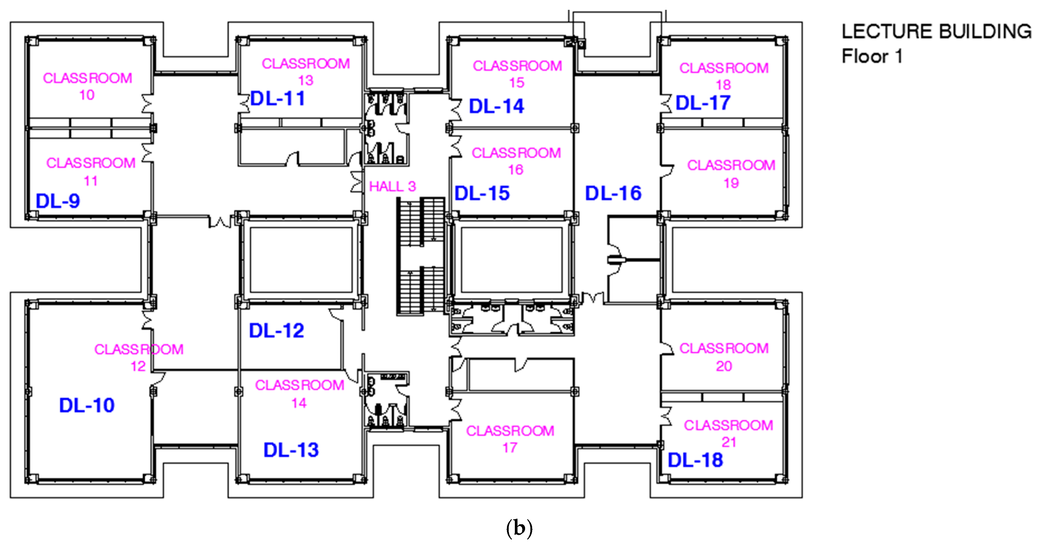
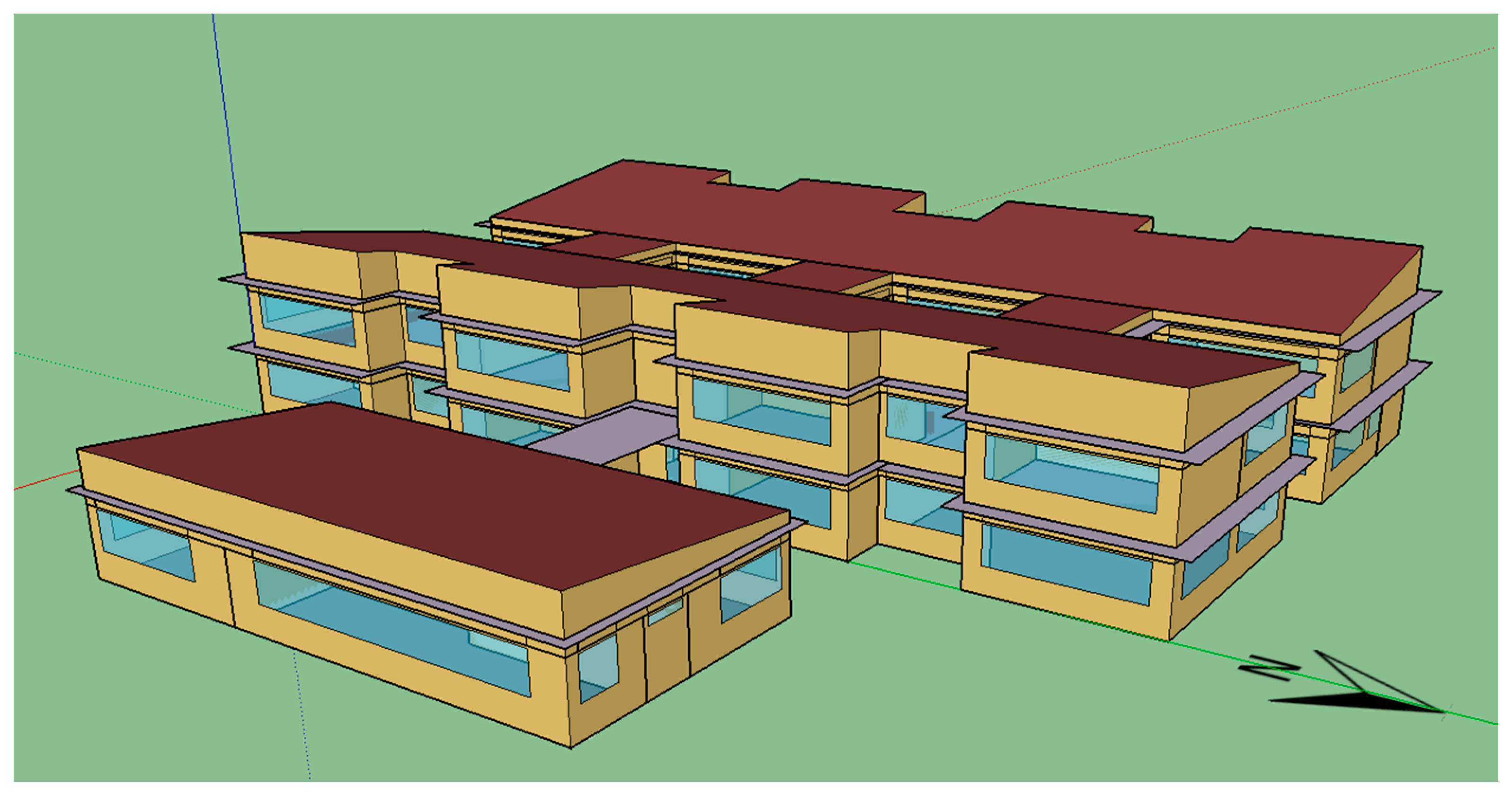
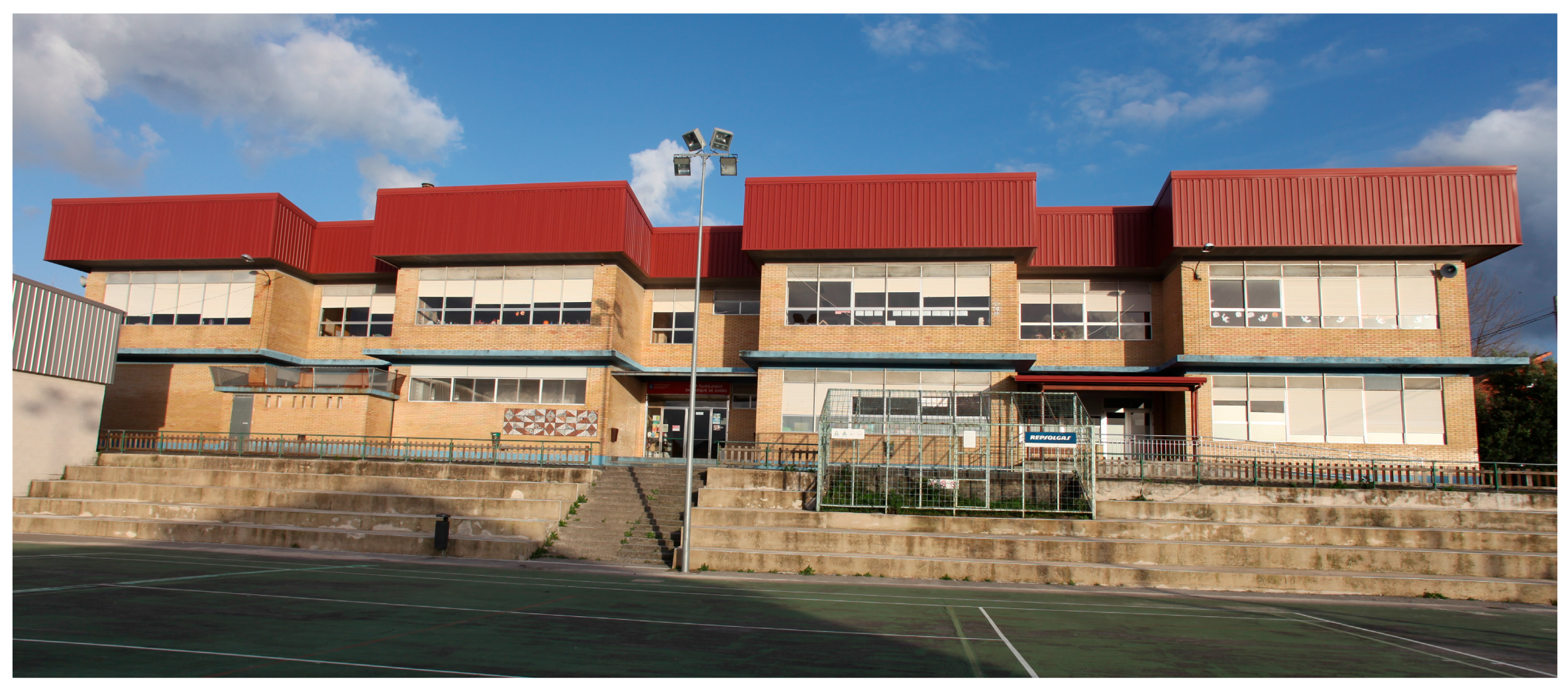
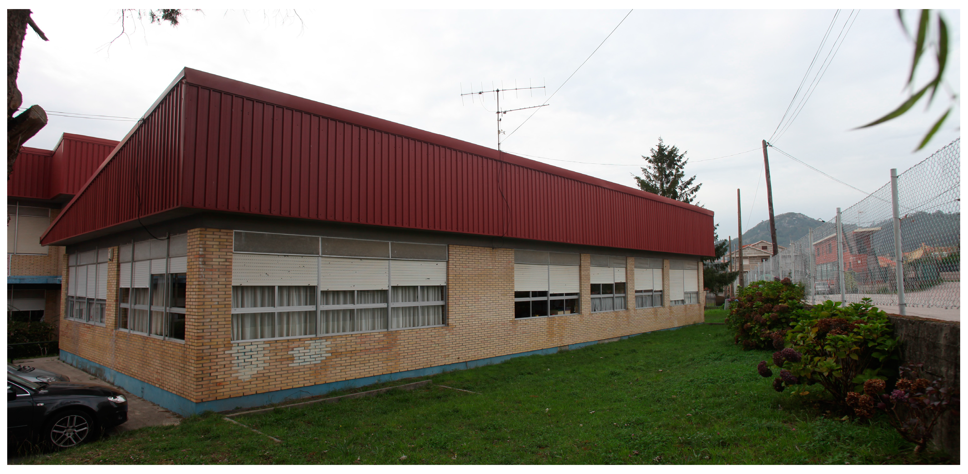
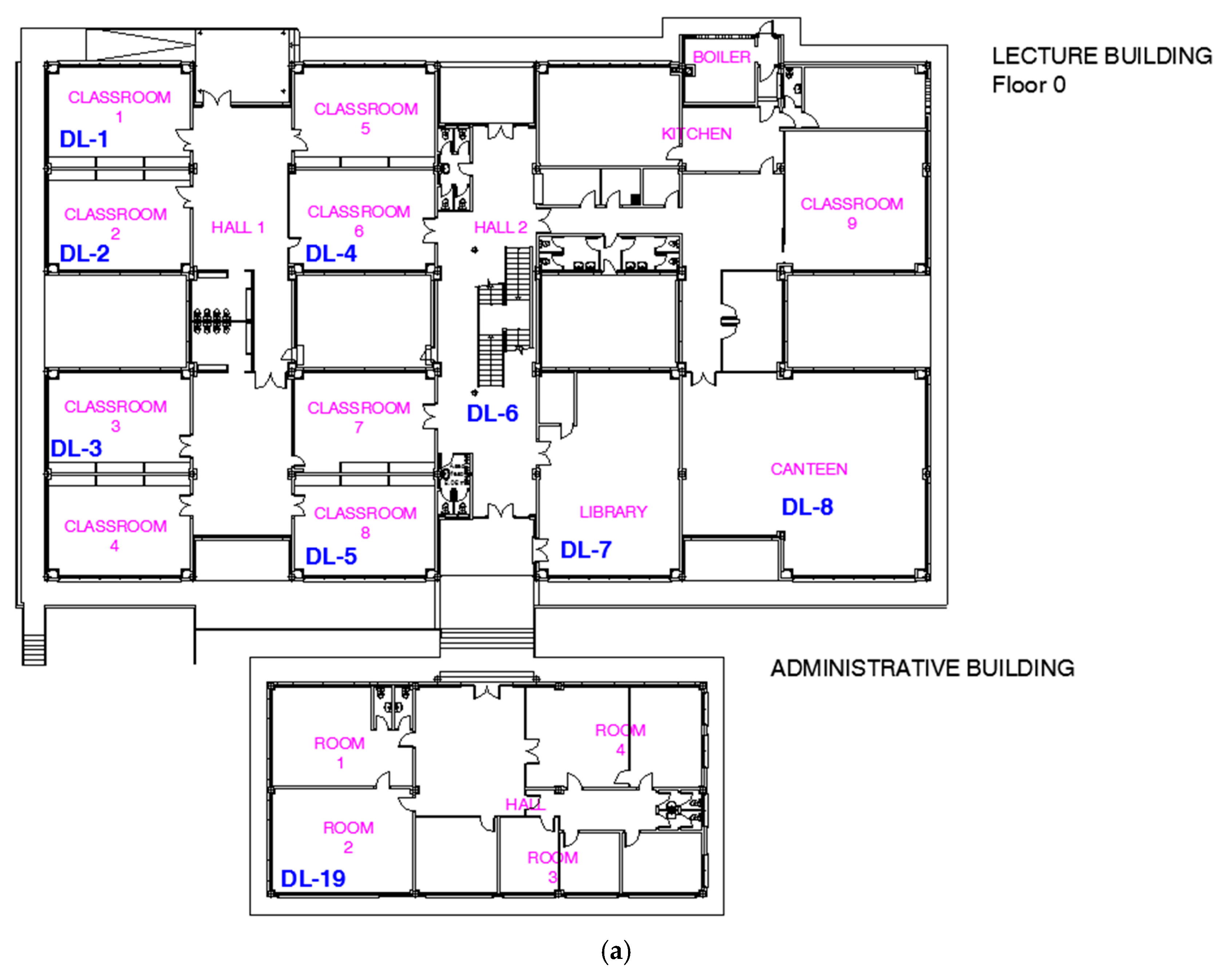
2.1. Building Description

The educational centre is composed of two principal buildings: the Lecture Building and the Administrative Building. In addition to these, there are other auxiliary buildings—sports centre, gymnasium and concierge—which were not considered in this study, since their thermal consumption is considered to be negligible.

The Lecture Building, which is shown in Figure 1, is composed of a ground and first floor laid out in a comb-shaped plan with two bodies communicated by three corridors that delimit two interior courtyards. The ground floor (inside area of 1209.06 m²) is intended for children's education (southern half) and common services (northern half), such as the dining room, kitchen, library, boiler room, etc. The upper floor (inside area of 1189.61 m²) is entirely dedicated to primary education.

In Figure 2, the Administrative Building is depicted. It faces the east façade of the Lecture Building. The inside area of this building is 292.84 m². It houses offices that are predominantly individually used as well as rooms for multiple use. It is primarily used in the mornings, according to the schedule of the centre.

The heating system common to both buildings is a fuel boiler, model Roca NTD 165, which is located in the Lecture Building, and steel plate radiators. The regular use of the centre, which receives 400 students, takes place in the morning, between 9:25 and 14:25. It has a canteen service from 14:30 to 15:30 and extracurricular activities from 16:00 to 17:00.

Both the Lecture and Administrative buildings are considerably old. They were built during the 1970s, as mentioned previously, and despite the fact that some specific reforms have been undertaken during this time, they are generally in a very deteriorated condition. The most serious problems that affect the majority of the energy consumption are due to poor insulation of both the windows, which have simple metal woodwork without thermal breaks, and blind boxes.

2.2. Temperature Monitoring

During the energy audit conducted during the 2014–2015 academic term, the buildings under study were monitored every ten minutes, with special prevalence during the cold season. For comfort requirements as well as the number of users, the Lecture Building analysis was prioritized. Thermohygrometers were used for recording indoor temperature and humidity data of the thermal zones, and the thermohygrometer characteristics are given in

Table 1. Thermohygrometer characteristics.

Characteristics	Temperature Sensor	Humidity Sensor
Resolution	0.1 °C	0.1% RH (relative humidity)
Accuracy	±0.5 °C	±2.5% RH (+5% to +95% RH)
Manufacturer: Testo; Model: 625

.

Initially, a first assessment of the interior conditions was made with point measurements in classrooms and other rooms. The selection of monitoring locations was made based on the conclusions obtained from the analysis of the point measurements and with the aim of covering the greatest typological diversity of spaces. That is why classrooms with a variety of position and window orientations, different floors and locations in the building were chosen. Likewise, characteristic spaces with special regimes of use, such as the canteen or the library, were studied. Conditions were analyzed in more open spaces, such as distributors, and sensors were placed in unheated areas, such as in false ceilings and below deck.

During the first month of the audit, between 15 October and 13 November, 19 registration points were taken, 18 of them in the classroom and one in the administrative building. From 13 November to 17 December, 10 points were monitored from those in the Lecture building. The planes in Figure 3 show the spaces where the data loggers (DL) were installed, which were placed centred in each room and close to the ceiling.

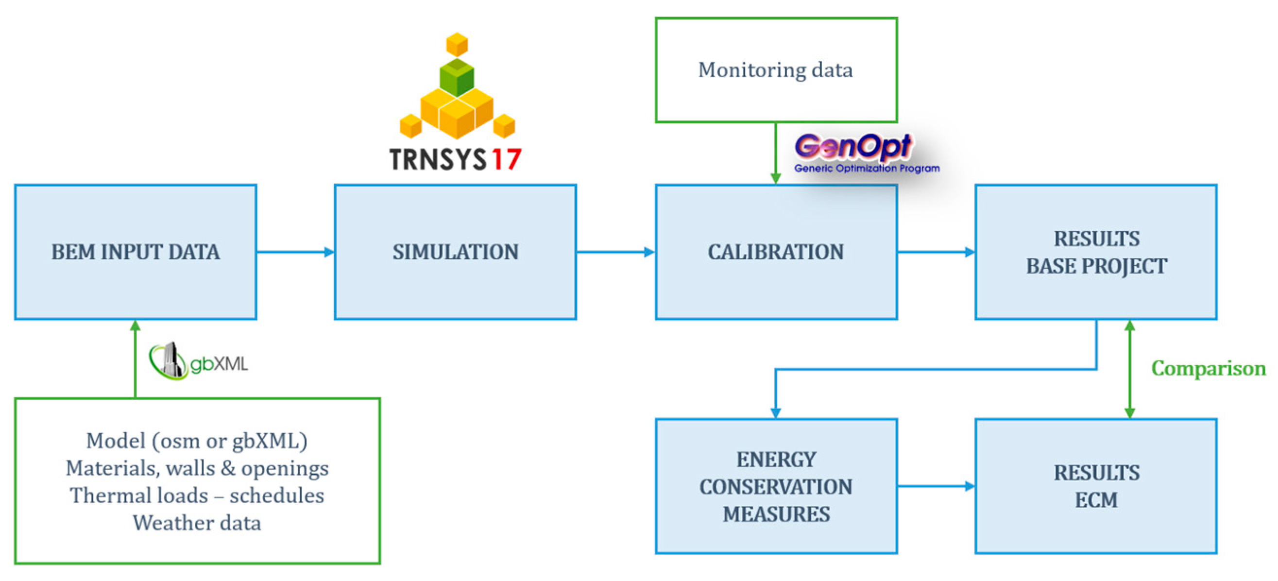
3. Simulation Methodology

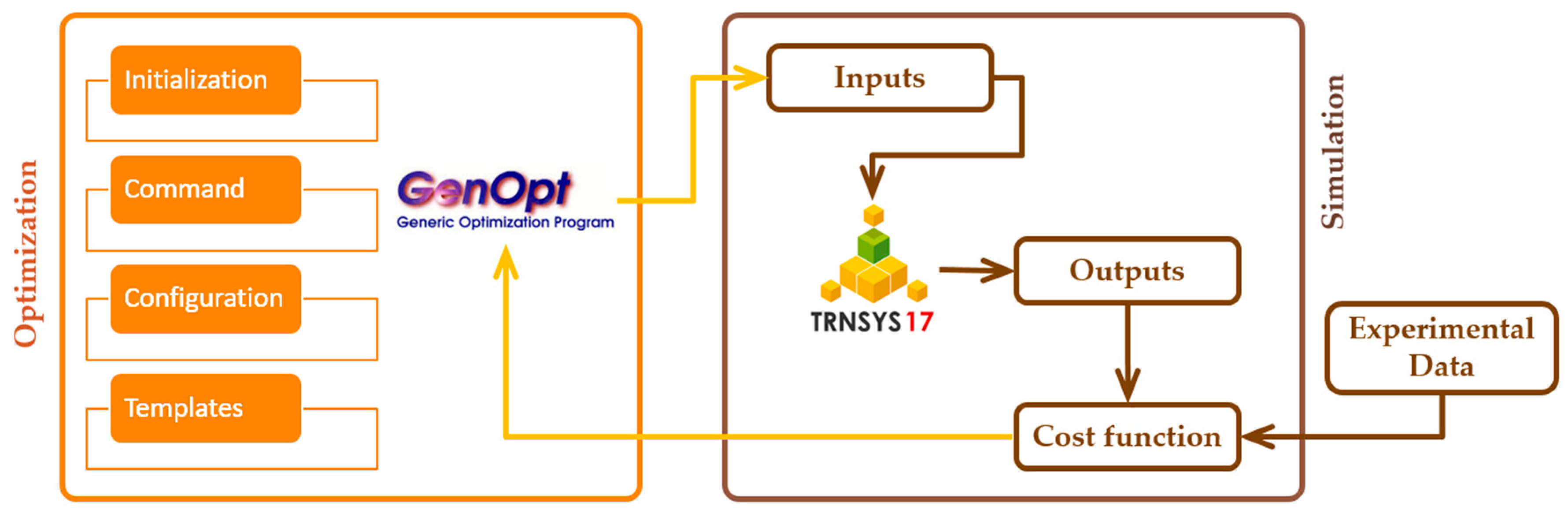
3.1. Simulation Software

The simulation software employed in this work was BCORE, a BEPS tool that was self-developed. It is an advanced technological solution that enables the automated calibration of simulations. The new tool is powerful and facilitates the introduction of data and the fulfilment of the building model, decreasing the costs of deployment for the modeller. Using a holistic approach, this software integrates into a single tool multiple utilities and applications that were previously not commercially combined: modelling, simulation, calibration, and the implementation of energy conservation measures (ECMs) in buildings. In addition, BCORE has a friendly framework that is easily usable by any end-user who may not necessarily be an information technologies expert.

The calculation engine chosen with which BCORE works is TRNSYS, which was developed by the University of Wisconsin, Madison, WI, USA. The software operation is based on introducing a building model, its geometry and enclosures, as well as its thermal loads, as discussed in the following section. These building data as well as weather data are necessary to run the simulation. However, the first simulations do not usually generate realistic results. At this point, this software provides its main contribution, which is the ability to calibrate the simulation to obtain a solution that is as close to reality as possible. Monitoring data are necessary to implement this calibration. Another strength of the program is the capability to define different ECMs and to compare them with the base project. The BCORE operational diagram is shown in Figure 4.

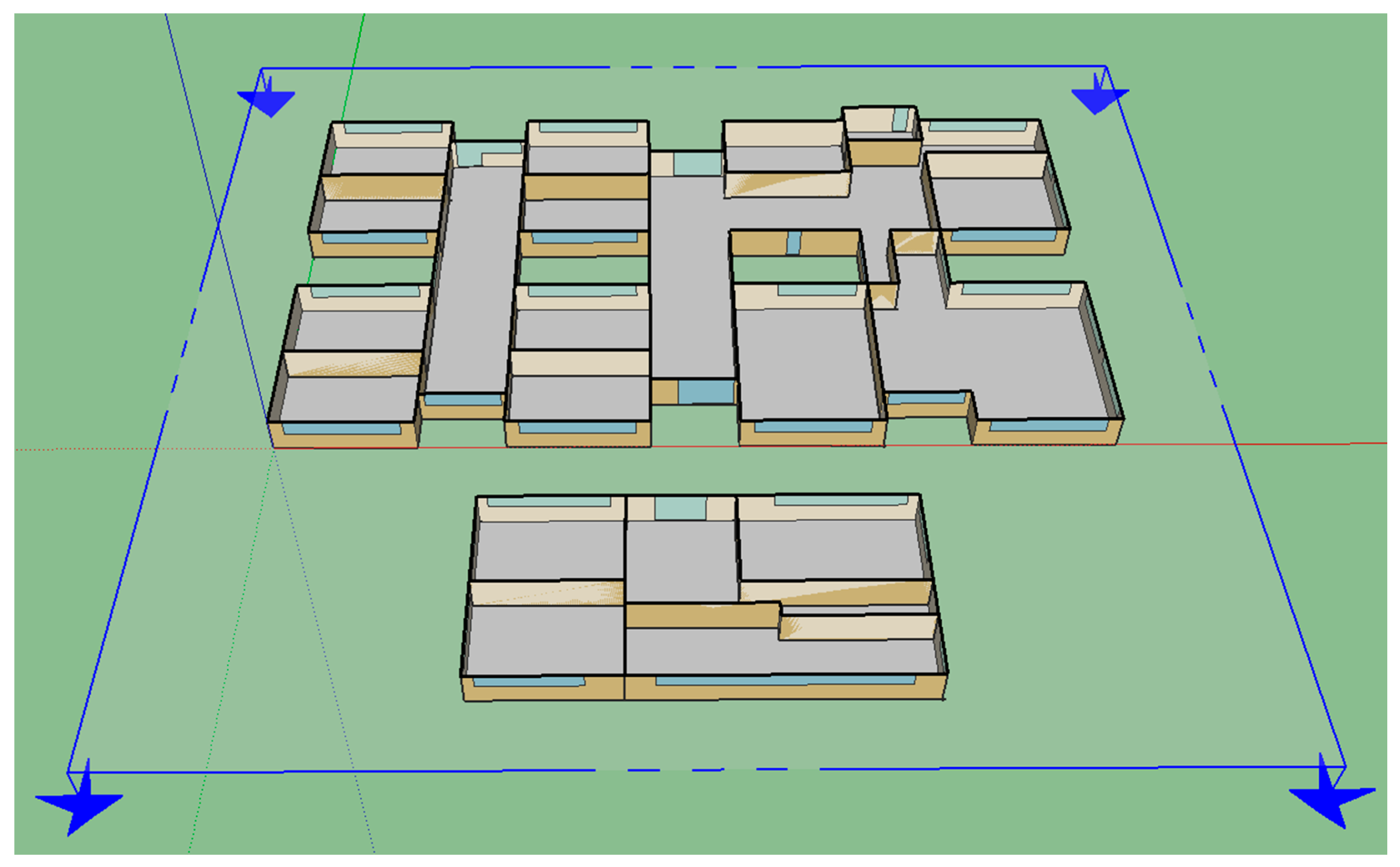
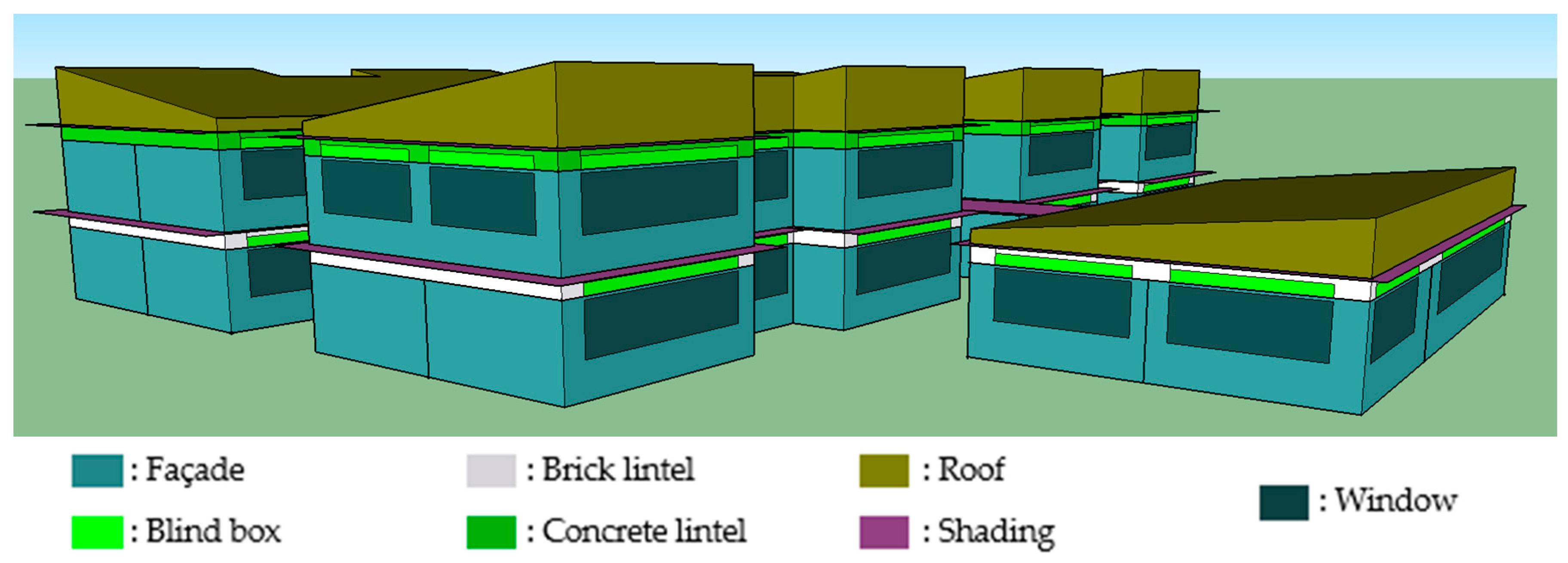
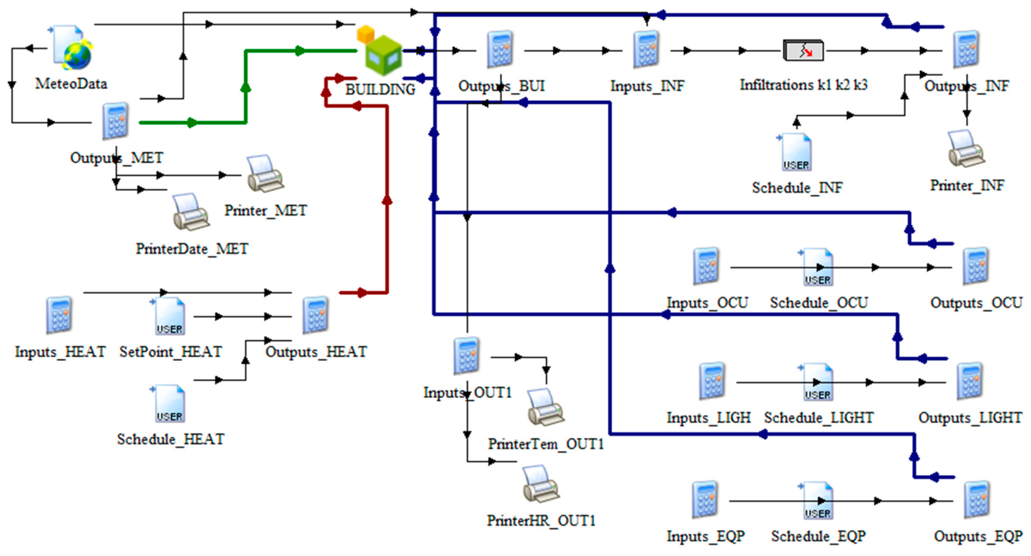
3.2. Model Description

The model of the school was created using the SketchUp software, in conjunction with the OpenStudio-Plugin, which allows the generation of a building geometry from scratch as well as the introduction of extra information that is used later in the simulation. An osm file with the generated geometry was produced and then imported into BCORE, which, once the construction and operational properties have been entered, will be transformed into the format necessary for TRNSYS to execute the dynamic simulation. Figure 5 shows the developed thermal model. As shown, the administrative building is facing east, and the overhanging roof and cornices were designed as solar shadings.

To simplify the model without impairing the precision required for the thermal simulation, similar rooms and classrooms were combined to minimize the number of thermal zones, neglecting the thermal inertia of the interior walls between combined spaces. Likewise, the spaces between the upper floor and the roof, despite being non-inhabited areas, were considered as additional non-conditioned thermal zones. Thus, the total number of thermal zones is 38 zones: 31 in the Lecture Building and 7 in the Administrative Building. In the model presented in Figure 6, a section of the ground floor is shown, where the thermal zones defined can be distinguished.

To define a constructive model of the school, visual inspections of the buildings were conducted and measurements of thermal transmittance were taken in those elements where it was possible. The thermal transmittance measures were made during the audit, using specialized equipment: a multifunction meter—model testo 435—together with a temperature probe for U-value calculation—model testo 635. The different constructive elements of the building were defined in the BCORE tool from the layer composition of each construction type to the thermal characteristics of each layer, i.e., heat capacity (J/kg·K), conductivity (W/m·K) and density (kg/m³) of the material. In Figure 7, these constructions can be differentiated, and their properties are summarised in

Table 2. Constructive characteristics of the building.

Construction	Total Thickness [m]	Total U-Value [W/m2·K]	Material	Thickness [m]	Conductivity [W/m·K]	Thermal Resistance [m2·K/W]
Façade	0.21	3.18	Brick fired clay ½ foot	0.10	0.667	-
			Air chamber	-	-	0.035
			Brick fired clay ½ foot	0.10	0.667	-
Blind box	0.04	4.45	Plywood	0.04	0.178	-
Brick lintel	0.22	3.03	Brick fired clay ½ foot	0.22	0.667	-
Concrete lintel	0.62	3.71	Reinforced concrete	0.62	2.300	-
Roof	0.08	6.73	Asbestos cement board	0.01	0.470	-
			Metal sheet	0.07	0.55	-
Horizontal partition	0.28	2.87	Mortar light aggregate	0.03	0.410	-
			Unidirectional slab ceramic	0.25	0.908	-
Vertical partition	0.10	6.67	Brick fired clay ½ foot	0.10	0.667	-
Slab	0.28	2.87	Mortar light aggregate	0.03	0.410	-
			Unidirectional slab ceramic	0.25	0.908	-

for the walls and in

Table 3. Characteristics of the openings of the building.

Buildings	Layers (-)	U-Value (W/m2·K)	g-Value (%)	Area Frame/Window (%)
Window glass	Simple (6 mm)	5.96	0.850	-
Window frame	-	5.70	-	15

for the openings.

3.3. Weather File

The weather data used in this study were taken from the MeteoGalicia [25] database for the location of the educational centre and were adjusted by interpolation of meteorological stations near the school with data from the last 10 years, so it was possible to generate a representative typical meteorological year (TMY). The data were converted to the energy plus weather (EPW) data format required by the meteorological data processor of TRNSYS. Previously, for the calibration phase, actual data from the meteorological stations of MeteoGalicia were used for the days in which the measurements of indoor humidity and temperature was performed, since actual meteorological data was required to validate the simulation.

3.4. Simulation

Figure 8 shows a diagram of the model simulation in the graphical interface of TRNYS. The main part of the diagram is the type 56 (BUILDING in the figure), which represents the building geometry and construction elements. It also includes the components that process the meteorological data (Type 15, MeteoData), and all of the internal loads that must be taken into account in the simulation: occupancy, lighting, infiltrations, etc. The building was simulated for an entire year (2014), since that was when the measurement campaign was undertaken, and there was a simulation step of 1 h.

Considering that BCORE automatically generates this simulation scheme, the program’s user does not need to generate it or work with it later because, as mentioned, the advantage of the software is that it allows the use of a powerful calculation engine, such as TRNSYS, without the necessity of an expert user.

Operational Conditions

As mentioned previously, there is some information that was introduced automatically into the BCORE software with external files, such as the geometry or the weather data. However, there is much information that was introduced internally in the software using its interface, such as the constructions previously exposed and the thermal loads and, in particular, the infiltrations, occupancy, lighting and equipment.

To determine the occupancy loads, according to ISO 7730:2005 [26], the activities of the people at the centre was considered for the teachers standing and light work activity, corresponding to a metabolic rate level of 90 W/person of sensible heat and 95 W/person of latent heat. For students, it was considered to be light activity with sitting and writing, corresponding to a metabolic rate of 65 W/person of sensible heat and 55 W/person of latent heat. Several authors studied thermal comfort parameters for children in classrooms [27,28,29], coming to the conclusion that the metabolic rate for children must be adjusted from that determined for adults. Children’s age is very important for the metabolic rate, as it depends on the children’s body surface area. Havenith [30] analyzed that area in children aged between 9 and 18, ranging from 1.23 m² to 1.96 m², with the body surface area for adults being 1.7 m². Since the studied buildings are a primary and elementary school, where the students are 6–12 year old children, in this work a reduction coefficient of 0.5 was applied for children´s metabolic rate [31].

The overall schedule of the centre is from 9:00 a.m. to 5:00 p.m. from Monday to Friday. Lessons are delivered according to the school calendar all year except on Christmas, Easter and during summer holidays (from mid-June to mid-September).

Practically, the entire centre is lighted with the same type of fluorescent luminaires, both in the form of conventional tubes and in the form of compact equipment. In this work, it was considered that 40% of the lamp power of the fluorescent tubes corresponded to the convective part and 60% corresponded to the radiant part.

For an estimation of the thermal load due to existing equipment, an average of approximately 1500 W was considered in each classroom during school days. Thus, 300 W of continuous load was taken during 5 h of lessons. In some classrooms, the power from an additional 1700 W heater was added for the winter months.

The infiltration values of the thermal zones were calculated in accordance with the empirical method proposed by the ASHRAE [32] K₁, K₂, K₃ model, which imply an accurate method for obtaining quick infiltration computations. Hence, the infiltration calculation—air changes per hour (ACH)—in each thermal zone was performed for each simulation step according to the Equation (1):

$$ACH=K_1+K_2·\left(T_{Zone}-T_{ambient}\right)+K_3·W_{\mathrm{s}},$$

(1)

where K₁ is the constant coefficient, K₂ is the temperature coefficient, K₃ is the wind speed coefficient and W_s is the wind speed. These coefficients were determined based on the construction level of the zone where the infiltration was calculated. Taking into account the previously mentioned poor insulation conditions of both buildings, the coefficients employed in this work were those recommended by ASHRAE for “Evidence of poor construction on older buildings where joints have separated”. In addition, to consider the entrance and exit of air due to the aperture of doors during the use of the school centre, a schedule from 9:00 to 17:00 hours was applied to the calculated infiltrations, which matches to the daytime hours when the buildings are inhabited. The calculated values for the infiltrations ranged from 0.19 ACH (obtained in classroom 6), to 0.83 ACH (obtained in the canteen).

Since the objective of this work is focused on the process of simulation and calibration of a building, (mainly its thermal envelope and operating conditions, and not so much the energy production and distribution facilities), to calculate the heating demands, an ideal heating system was established that ensures compliance with the internal comfort conditions for the users, i.e., students and teachers. An ideal system was defined that maintains the indoor temperature at 20 °C in the classrooms and at 18 °C in the corridors, halls and administrative areas during school hours, starting from 8:00 a.m. and ending at 12:00 a.m. This was established for the period between 1 November and 31 March, except for the Christmas holidays.

3.5. Calibration

Although the calculation engine has been proved to give successful results for building simulations, the model must be adjusted in accordance with the actual behavior of the building. With this aim, a calibration of the simulation was performed to achieve the requirements established by ASHRAE Guideline 14 [22] to consider the buildings calibrated. The methodology employed during this process is described in this section.

A deterministic methodology was applied in the calibration process. This method works by changing a number of parameters, which can be continuous or discrete, and by searching for the minimization of an objective function that measures the differences between the model predictions and the measured data. The cost function, which was considered to be minimized in this work, was the coefficient of variation of the root mean square error, CV(RMSE), as defined in Equation (2). Later, in regard to the validation of the obtained results, another metric proposed by ASHRAE Guideline 14 was used, which is the normalized mean bias error (NMBE), as defined in Equation (3):

$$\mathrm{CV}\left(\mathrm{RMSE}\right)=\frac{\sqrt{{{\displaystyle \sum }}_{i=1}^n{\left(T_{sim}-T_{real}\right)}^2}/n}{\overline{T_{real}}},$$

(2)

$$\mathrm{NMBE}=\frac{{{\displaystyle \sum }}_{i=1}^n\left(T_{sim}-T_{real}\right)/n}{\overline{T_{real}}}$$

(3)

where:

• $T_{sim}$ is the simulated indoor air temperature of the zone;
• $T_{real}$ is the registered real temperature;
• $\overline{T_{real}}$ is the average registered real temperature;
• n is the number of data.

As explained in Section 2.2, measurement campaigns were performed. Temperature data from 15 October to 24 December were used in this work to calibrate the model by comparing this experimental data (T_real in Equation (2)) with the indoor temperature predicted by the simulation software, or T_sim, in the same thermal zone. The registered data were acquired in ten-minute intervals, and the simulation step was one hour; hence, the temperature data were previously pre-processed so that they could be properly compared. The temperature data used correspond to data-loggers positioned in 19 different zones in the buildings, as shown in Figure 3. The cost function was calculated as the mean CV(RMSE) value, as defined above, in each zone, as shown in Equation (4). Similarly, the NMBE total for the building was calculated according to Equation (5):

$$\mathrm{CV}{\left(\mathrm{RMSE}\right)}_{\mathrm{total}}=\frac{{{\displaystyle \sum }}_{\mathrm{k}=1}^{{\mathrm{n}}_{\mathrm{z}}}\mathrm{CV}{\left(\mathrm{RMSE}\right)}_{{\mathrm{Z}}_{\mathrm{k}}}}{n_Z}$$

(4)

$${\mathrm{NMBE}}_{\mathrm{total}}=\frac{{{\displaystyle \sum }}_{\mathrm{k}=1}^{{\mathrm{n}}_{\mathrm{z}}}{\mathrm{NMBE}}_{{\mathrm{Z}}_{\mathrm{k}}}}{n_z}$$

(5)

The optimization software selected to perform the calibration was GenOpt 3.0.1. [33], which executes the Hooke-Jeeves implementation of the generalized pattern search (GPS) algorithm, a hybrid algorithm for global optimization. Using this algorithm, the parameters that are calibrated are varied within pre-set limits, during a series of iterations.

Thus, the developed software is an innovation in the field of energy simulation because it allows for the automated calibration of the model. Because of the BCORE tool, this calibration software is executed in a simple and semi-automated way. The first steps are performed manually since the user needs to define which parameters should be calibrated (parameters selected for this work will be discussed below) and provide the program with the available monitoring data, which are either the thermal demand or hygrometric conditions (temperature or humidity) within the thermal zones. Once these parameters have been defined, BCORE autonomously and automatically executes the two programs involved in the calibration process. For each GenOpt iteration, TRNSYS performs a new simulation with the set values for each variable. Then, the objective function is calculated to check if it decreased in comparison with the previous step. The optimum result is considered to have been achieved when equal values are found during five consecutive iterations. Figure 9 shows the interaction diagram between TRNSYS and GenOpt during the calibration process.

As previously stated, the buildings are in poorly maintained conditions, with defective insulation at both the window frames and blind boxes. This makes infiltrations an important focus of thermal energy loss, which are difficult to quantify. Hence, the parameters that were taken into account for calibration were those corresponding to the infiltrations, which were the part of the model that was defined with less precision, since the audit that was performed provided much information on the construction and operation characteristics of the buildings. Thus, the parameters proposed for calibration are those indicated in

Table 4. Calibration parameters.

Parameter	Description
Infiltration 1	Infiltrations below deck in both buildings
Infiltration 2	Infiltrations in the false ceilings
Infiltration 3	Infiltrations in the classrooms
Infiltration 4	Infiltrations in zones in the Administrative Building
Infiltration 5	Infiltrations in the halls of both buildings

which are dimensionless multipliers applied to the infiltrations calculated according to Equation (1) at each simulation step. The 38 thermal zones were put into 5 different infiltrations groups, so 5 infiltration multipliers (one common for each group) needed to be calibrated, as shown in Table 4, decreasing the need for computations by reducing the degrees of freedom without significantly decreasing the optimization capacity.

To calibrate these parameters, it is necessary to delimit the ranges between which they can be varied. Since the parameters are multipliers of the instantaneous infiltration values, the initial value for each parameter is 1, and the lower and upper limits for all of them are 0.2 and 10, respectively.

4. Results and Discussion

The results obtained during the study described in this paper are introduced in this section. First, the outcomes of the calibration process and the accuracy of the model are presented, and then the behavior of the model is shown in graphs that compare the calibrated and uncalibrated simulations.

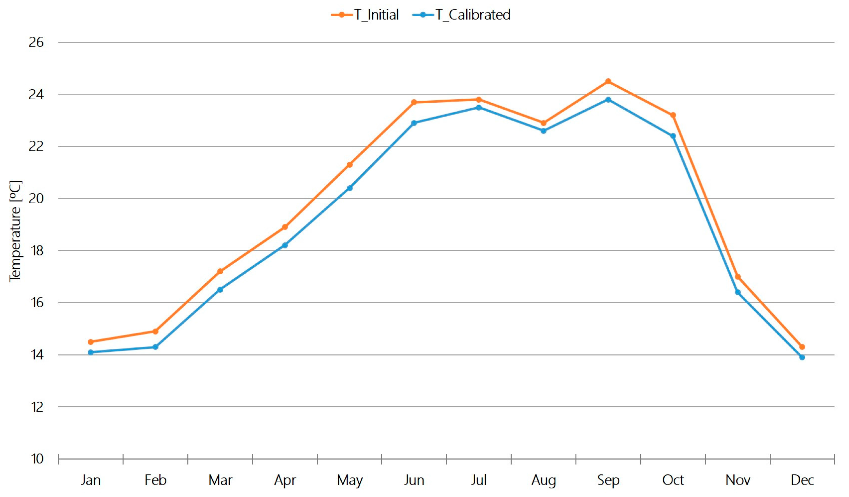
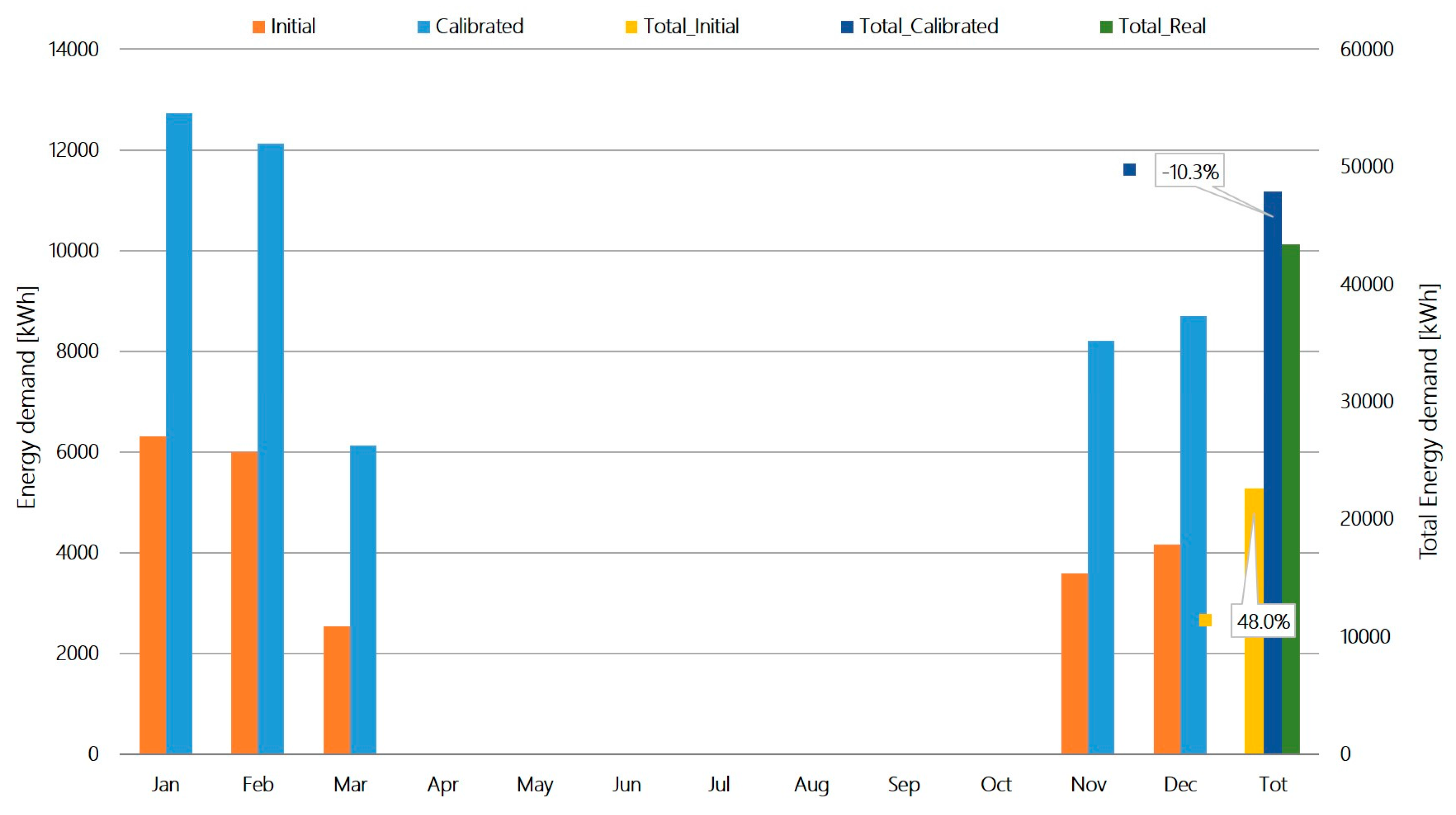
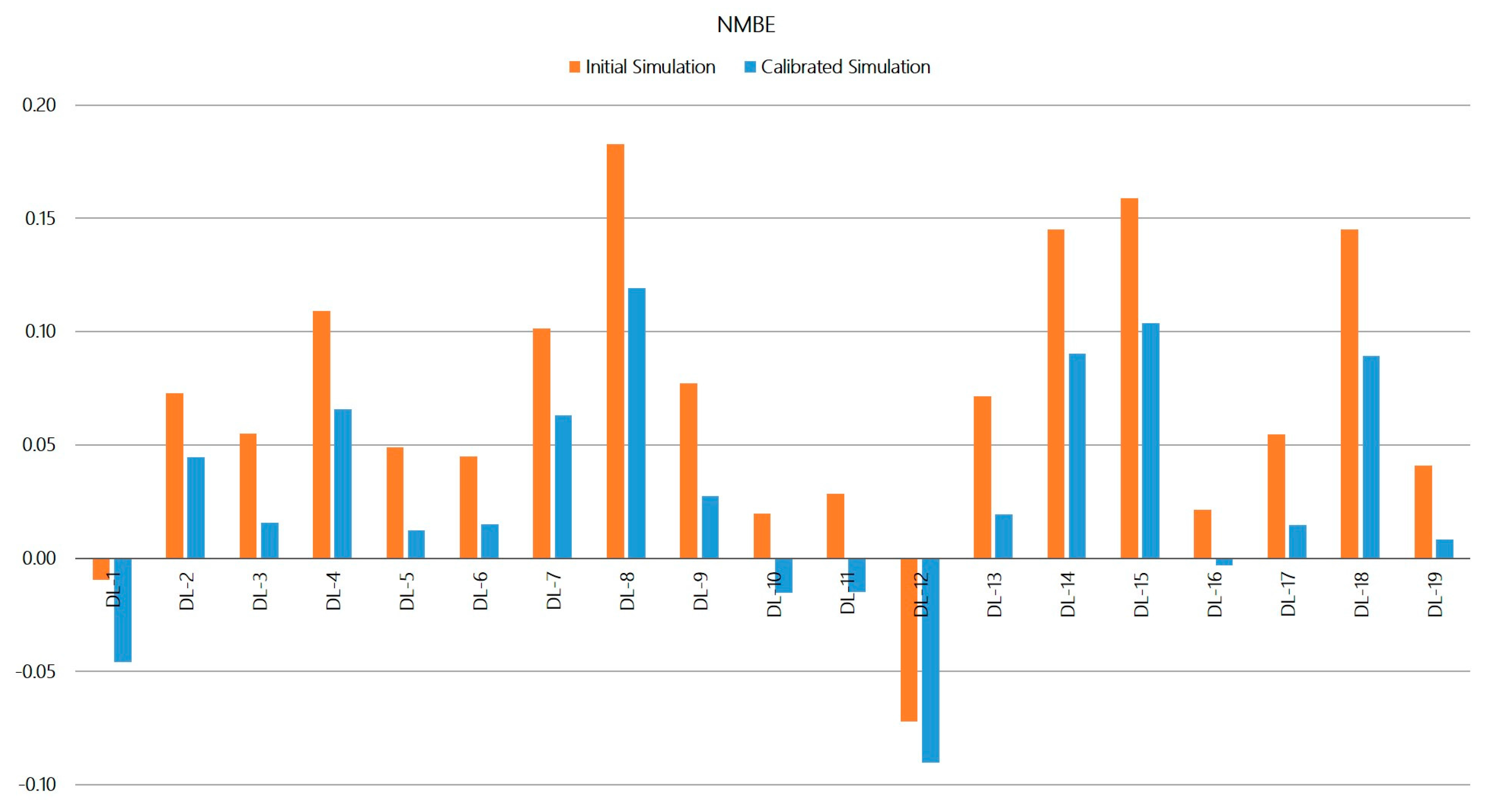
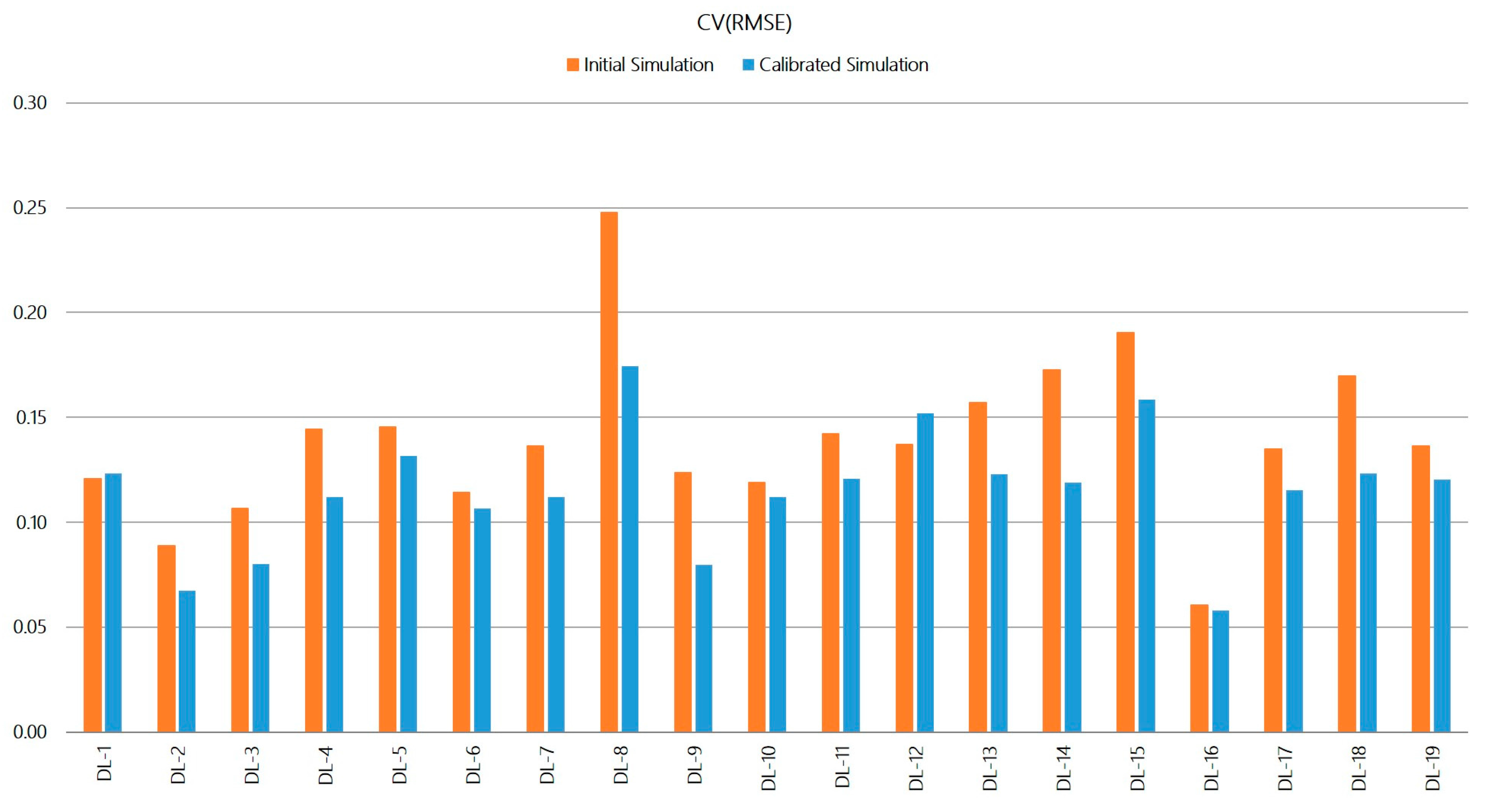
4.1. Calibration Results

After 125 iterations and 2 computer hours on a PC with an INTEL CORE I7 processor and 16 gigabytes of random access memory (RAM), the applied method achieved the minimum value of the defined cost function. As demonstrated in the validation of the model described in the following section, the starting simulation was a correct model, and it was difficult to optimize due to its high initial accuracy.

However, according to the calibration results obtained, the infiltration model K₁, K₂, K₃ defined by the ASHRAE, which takes into account difference in pressures, densities and temperatures between the external air and the interior, is a model that can be used for this simulation, since the obtained multipliers are within a range of values that can be considered acceptable.

Table 5. Calibrated values of the selected variables.

Parameter	Calibrated Value
Infiltration 1	0.2
Infiltration 2	0.2
Infiltration 3	10
Infiltration 4	9.3
Infiltration 5	5

shows the dimensionless multipliers obtained through the calibration process that were applied to the infiltrations of each group of zones that were calculated according to K₁, K₂, K₃.

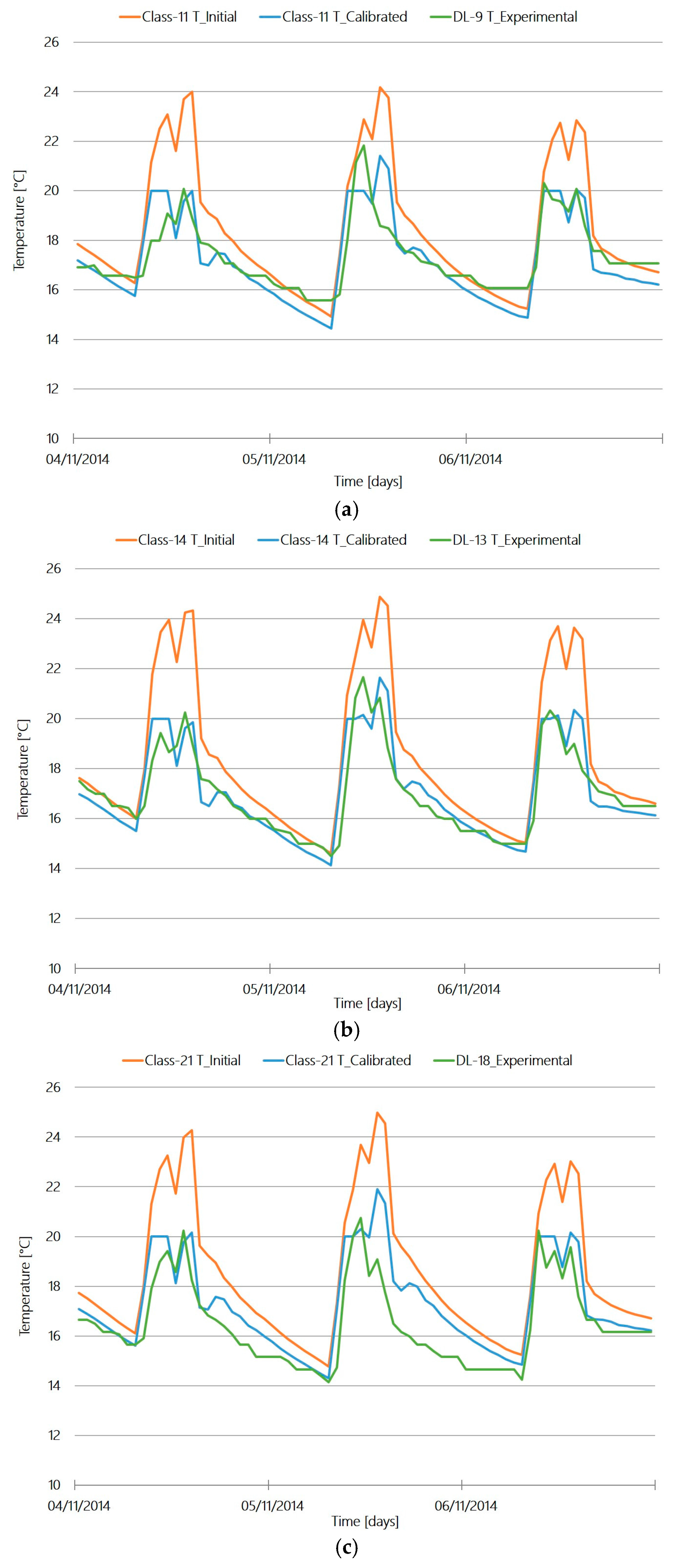
4.2. Model Validation

To assess the accuracy of the simulation, the ASHRAE Guideline 14 criteria was followed, which states that an entire building can be considered calibrated when the computer model has a NMBE of 10% and a CV(RMSE) of 30% when the data sampling period is hourly, as in the simulation in this work. These metrics of the simulation were calculated using Equations (2)–(5).

Figure 10 and Figure 11 represent the NMBE and CV(RMSE), respectively, before and after the calibration for each of the thermal zones that were considered in the calibration process for a period of two months. As shown in the plots, the simulation errors after calibration were highly reduced. The NMBE ranged from −7.21% to 18.29% for the initial simulation, and it decreased to the range of −9.02% to 11.92% in the calibration model. On the other hand, CV(RMSE) decreased from an initial range of 6.06% to 24.75%, to a range of 5.81% to 17.45%. The x-axis in both figures correspond to the sensor identifier previously defined in Figure 3 in Section 2.2.

In

Table 6. Statistical error indices before and after calibration of the simulation.

Error	Initial Simulation	Calibrated Simulation	Reduction
NMBE	6.82%	2.73%	59.97%
CV(RMSE)	13.93%	11.52%	17.27%

, the performance metrics that were calculated as the mean in each zone are presented, and again we compared the uncalibrated simulation with the calibrated one. The uncalibrated simulation already presents a reasonable level of accuracy, meaning that the initial model was a suitable representation of the actual building. However, after the process of calibration, the simulation error decreased by approximately 60% in NMBE and by approximately 17% in CV(RMSE).

As an example of the accuracy of the model, the plots in Figure 12 show the values of the three indoor air temperatures, namely, the registered experimental value, T_experimental, the initial uncalibrated simulation value obtained, T_initial, and the value of the calibrated simulation, T_calibrated. They are graphed for a short period of time (3 days) from the 4th to the 6th of November so the differences between the three curves can be clearly seen. Upon analyzing the graphs presented, it is verified that the calibrated model certainly has a high degree of accuracy, improving the results of the indoor air temperature predicted by the initial simulation. As shown in the three plots, the initial simulation reached temperatures that were approximately 2 °C above the experimental, whereas the maximum temperature of the calibrated model was near the actual value. However, during the period in which the indoor temperature decreased when the building was not in use, the lower values in the three curves are reasonably similar.

Figure 13 represents the monthly temperature profile predicted with the simulation program for the year of 2014. The uncalibrated model produced outcomes that were slightly higher than the calibrated simulation. The plots show that January and December are the months with the lower temperatures, which is consistent with reality since they are the coldest months in the region where the school centre is located. Furthermore, there was a decrease in the temperature during August compared with July or September, which is explained because this is a month without teaching hours in which neither building is occupied.

In this case study, energy consumption data from invoices were not available, and the only accessible data was the value of litres of fuel consumed annually in the school, which was practically unchanged over the years, approximately an average of 5000 L. With this average annual fuel data and taking into account, as previously defined, that they had a fuel boiler with a 0.87% efficiency and the fuel low heating value (LHV) was 9.98 kWh/L the average annual consumption of the school was 43,413 kWh. In Figure 14, the monthly thermal demand profiles calculated in the simulation, both with the initial and the calibrated model, can be graphically compared. The total energy demand is also represented in the last column of the figure, including labels quantifying the percentage error with regard to the actual demand value that, as shown, improves with the calibration from 48% lower to 10% higher.

5. Conclusions

In this research, the energy performances of buildings forming a school centre in the northwest of Spain were analyzed, which were considered a particularly complex case since they are old buildings in a poor state of maintenance, turning into a big challenge to model and simulate it in a reliable way. For this purpose, a transient simulation of the building energy model of the school was conducted using TRNSYS, which is a commercial software with proven reliability in the field of thermal simulations.

Calibration of the computer model plays a crucial role. A deterministic calibration approach was applied to the initial model of the building. The results showed that a trustworthy calibration process was performed since the metrics employed to verify the error showed a reduction of approximately 60% in NMBE and 17% in the CV(RMSE).

The procedure proposed was proven to be successful because the outcomes of the calibrated simulation produced a narrow error. The final NMBE was 2.73% and the CV(RMSE) was 11.52% for the tested period, proving that an accurate model of the actual school was achieved. Therefore, the joint use of TRNSYS and the deterministic calibration method that GenOpt executes constitutes a useful methodology for the assessment (using calibrated thermal simulations) of buildings in deteriorated conditions.

The methodology described was implemented using our ground-breaking tool, BCORE, which combines the calculation engine, TRNSYS, to run the simulations with GenOpt to execute the algorithm employed in the calibration process. As confirmed in this work, it is suitable software for acquiring calibrated building simulations.

References

1. Recast, E.P.B.D. Directive 2010/31/EU of the European Parliament and of the Council of 19 May 2010 on the Energy Performance of Buildings; Official Journal of the European Union (OJ): Brussels, Belgium, 2010. [Google Scholar]
2. Parliament, E. Directive 2012/27/EU of the European Parliament and of the Council of 25 October 2012 on Energy Efficiency, Amending DIRECTIVES 2009/125/EC and 2010/30/EU and Repealing Directives 2004/8/EC and 2006/32/EC; European Commission: Brussels, Belgium, 2012. [Google Scholar]
3. European Commsion. Available online: https://ec.europa.eu/energy/en/topics/energy-efficiency/buildings (accessed on 16 May 2017).
4. Martinez-Molina, A.; Boarin, P.; Tort-Ausina, I.; Vivancos, J.-L. Post-occupancy evaluation of a historic primary school in Spain: Comparing PMV, TSV and PD for teachers’ and pupils’ thermal comfort. Build. Environ. 2017, 117, 248–259. [Google Scholar] [CrossRef]
5. Nolte, I.; Strong, D. Europe’s Buildings under the Microscope; Buildings Performance Institute Europe (BPIE): Bruxelles, Belgium, 2011. [Google Scholar]
6. Pérez-Lombard, L.; Ortiz, J.; Pout, C. A review on buildings energy consumption information. Energy Build. 2008, 40, 394–398. [Google Scholar] [CrossRef]
7. Lam, J.C. Energy analysis of commercial buildings in subtropical climates. Build. Environ. 2000, 35, 19–26. [Google Scholar] [CrossRef]
8. Ma, Z.; Cooper, P.; Daly, D.; Ledo, L. Existing building retrofits: Methodology and state-of-the-art. Energy Build. 2012, 55, 889–902. [Google Scholar] [CrossRef]
9. Salvalai, G.; Malighetti, L.E.; Luchini, L.; Girola, S. Analysis of different energy conservation strategies on existing school buildings in a Pre-Alpine Region. Energy Build. 2017, 145, 92–106. [Google Scholar] [CrossRef]
10. Sekki, T.; Airaksinen, M.; Saari, A. Effect of energy measures on the values of energy efficiency indicators in Finnish daycare and school buildings. Energy Build. 2017, 139, 124–132. [Google Scholar] [CrossRef]
11. Congedo, P.; D’Agostino, D.; Baglivo, C.; Tornese, G.; Zacà, I. Efficient solutions and cost-optimal analysis for existing school buildings. Energies 2016, 9, 851. [Google Scholar] [CrossRef]
12. Pisello, A.; Bobker, M.; Cotana, F. A building energy efficiency optimization method by evaluating the effective thermal zones occupancy. Energies 2012, 5, 5257–5278. [Google Scholar] [CrossRef]
13. Crawley, D.B.; Hand, J.W.; Kummert, M.; Griffith, B.T. Contrasting the capabilities of building energy performance simulation programs. Build. Environ. 2008, 43, 661–673. [Google Scholar] [CrossRef]
14. Klein, S. TRNSYS 17—A Transient System Simulation Program User Manual; University of Wisconsin-Madison, Solar Energy Laboratory: Madison, WI, USA, 2012. [Google Scholar]
15. Ciulla, G.; Lo Brano, V.; D’Amico, A. Modelling relationship among energy demand, climate and office building features: A cluster analysis at European level. Appl. Energy 2016, 183, 1021–1034. [Google Scholar] [CrossRef]
16. Martínez-Ibernón, A.; Aparicio-Fernández, C.; Royo-Pastor, R.; Vivancos, J.L. Temperature and humidity transient simulation and validation in a measured house without a HVAC system. Energy Build. 2016, 131, 54–62. [Google Scholar] [CrossRef]
17. Cacabelos, A.; Eguía, P.; Míguez, J.L.; Granada, E.; Arce, M.E. Calibrated simulation of a public library HVAC system with a ground-source heat pump and a radiant floor using TRNSYS and GenOpt. Energy Build. 2015, 108, 114–126. [Google Scholar] [CrossRef]
18. Rey, G.; Ulloa, C.; Míguez, J.; Cacabelos, A. Suitability assessment of an ICE-based micro-CCHP unit in different Spanish climatic zones: Application of an experimental model in transient simulation. Energies 2016, 9, 969. [Google Scholar] [CrossRef]
19. Kim, Y.-J.; Park, C.-S. Stepwise deterministic and stochastic calibration of an energy simulation model for an existing building. Energy Build. 2016, 133, 455–468. [Google Scholar] [CrossRef]
20. Chae, Y.; Lee, Y.; Longinott, D. Assessment of retrofitting measures for a large historic research facility using a building energy simulation model. Energies 2016, 9, 466. [Google Scholar] [CrossRef]
21. Fabrizio, E.; Monetti, V. Methodologies and advancements in the calibration of building energy models. Energies 2015, 8, 2548–2574. [Google Scholar] [CrossRef]
22. Guideline 14-2002, Measurement of Energy and Demand Savings; American Society of Heating, Ventilating, and Air Conditioning Engineers: Atlanta, Georgia, 2002.
23. Cacabelos, A.; Eguía, P.; Febrero, L.; Granada, E. Development of a new multi-stage building energy model calibration methodology and validation in a public library. Energy Build. 2017, 146, 182–199. [Google Scholar] [CrossRef]
24. ENGINENCY. A Holistic System for Building Inspection and Energy Efficiency Management. Available online: http://www.enginency-project.eu/ (accessed on 16 May 2017).
25. MeteoGalicia. Available online: http://www.meteogalicia.gal/web/index.action (accessed on 16 May 2017).
26. ISO. Ergonomics of the Thermal Environment—Analytical Determination and Interpretation of Thermal Comfort Using Calculation of the PMV and PPD Indices and Local Thermal Comfort Criteria; ISO: Geneva, Sweden, 2005. [Google Scholar]
27. Mors, S.T.; Hensen, J.L.M.; Loomans, M.G.L.C.; Boerstra, A.C. Adaptive thermal comfort in primary school classrooms: Creating and validating PMV-based comfort charts. Build. Environ. 2011, 46, 2454–2461. [Google Scholar] [CrossRef]
28. Teli, D.; Jentsch, M.F.; James, P.A.B. Naturally ventilated classrooms: An assessment of existing comfort models for predicting the thermal sensation and preference of primary school children. Energy Build. 2012, 53, 166–182. [Google Scholar] [CrossRef]
29. Almeida, R.M.S.F.; Ramos, N.M.M.; de Freitas, V.P. Thermal comfort models and pupils’ perception in free-running school buildings of a mild climate country. Energy Build. 2016, 111, 64–75. [Google Scholar] [CrossRef]
30. Havenith, G. Metabolic rate and clothing insulation data of children and adolescents during various school activities. Ergonomics 2007, 50, 1689–1701. [Google Scholar] [CrossRef] [PubMed]
31. IDAE. Guía Técnica de Instalaciones de Climatización con Equipos Autónomos. Available online: http://www.idae.es/uploads/documentos/documentos_17_Guia_tecnica_instalaciones_de_climatizacion_con_equipos_autonomos_f9d4199a.pdf (accessed on 13 June 2017).
32. ASHRAE. ASHRAE Handbook of Fundamentals 1989, Chapter 22: Ventilation and Infiltration; ASHRAE: New York, NY, USA, 1989. [Google Scholar]
33. GENOPT. Generic Optimization Program. Available online: http://simulationresearch.lbl.gov/GO/ (accessed on 13 June 2017).
Figure 1. West façade of the Lecture Building.
Energies 10 00807 g001
Figure 2. East façade of the Administrative Building.
Energies 10 00807 g002
Figure 3. Location of sensors (DL-1 to DL-19) in the Lecture and Administrative Buildings: (a) Ground floor and (b) First floor.
Energies 10 00807 g003aEnergies 10 00807 g003b
Figure 4. BCORE operational diagram.
Energies 10 00807 g004
Figure 5. Thermal model of the school in SketchUp.
Energies 10 00807 g005
Figure 6. Section of the building model of the ground floor.
Energies 10 00807 g006
Figure 7. Constructive elements employed in the school model.
Energies 10 00807 g007
Figure 8. Building simulation diagram developed in TRNSYS simulation studio.
Energies 10 00807 g008
Figure 9. Interaction diagram for calibration with GenOpt and TRNSYS.
Energies 10 00807 g009
Figure 10. Normalized mean bias error (NMBE) for indoor temperature in each thermal zone with registered data.
Energies 10 00807 g010
Figure 11. CV(RMSE) for indoor temperature in each thermal zone with registered data.
Energies 10 00807 g011
Figure 12. Indoor air temperature with uncalibrated and calibrated simulation versus the experimental data for three thermal zones of the building: (a) comparison in Classroom 11 where data logger 9 was placed, (b) comparison in Classroom 14 with data logger 13 and (c) comparison in Classroom 21 with data logger 18.
Energies 10 00807 g012
Figure 13. Simulated average monthly indoor temperatures.
Energies 10 00807 g013
Figure 14. Monthly energy demand of the simulated building. Error in total energy demand in labels.
Energies 10 00807 g014