
Determining Switched Reluctance Motor Current Waveforms Exploiting the Transformation from the Time to the Position Domain


1
Department of Computer Engineering, Poznań University of Technology, ul. Piotrowo 3a, 60-965 Poznań, Poland
2
Electronics and Computer Science, University of Southampton, Southampton SO17 1BJ, UK
*
Author to whom correspondence should be addressed.
Energies 2017, 10(6), 799; https://doi.org/10.3390/en10060799
Submission received: 16 March 2017
/
Revised: 19 May 2017
/
Accepted: 5 June 2017
/
Published: 12 June 2017
Abstract
:This paper addresses the issue of estimating current waveforms in a switched reluctance motor required to achieve a desired electromagnetic torque. The methodology employed exploits the recently-developed method based on the transformation from the time to the position domain. This transformation takes account of nonlinearities caused by a doubly-salient structure. Owing to this new modelling technique it is possible to solve optimization problems with reference torque, constrained voltage, and parameter sensitivity accounted for. The proposed methodology is verified against published solutions and illustrated through simulations and experiments.
1. Introduction
Switched reluctance motors (SRM) are widely used in various applications due to their simple design and, consequently, attractive prices. The doubly-salient construction, however, causes the motor characteristics to be nonlinear [1,2] resulting in excessive torque ripples during motion. This unfavourable phenomenon is particularly noticeable with the simplest control method where the phase currents are switched on and off in sequence. Under such control the motor runs in open loop which is detrimental for stability, robustness, and performance. This provided the initial motivation for the authors to search for and develop more advanced control strategies.
To operate in a closed loop the SRM requires an electronic commutator. There exist two main trends in the design of such a device, but both rely on the knowledge of the torque profile versus position and current, although sometimes the current is deemed unimportant if saturation is neglected. The first approach is to search for such current waveforms which will assure a delivery of the required electromagnetic torque. The second method utilises the torque profile to estimate the electromagnetic torque, then the controller finds the associated torque error and either speeds up or slows down the magnetic flux.
A short review of previous attempts to resolve the issue now follows to provide the state of the art. The first published work on this subject was [3] where an electronic commutator was applied to linearize motor dynamics by a linearizing and decoupling transformation (LDT). The concept relies on a phase indicator which points at the single phase responsible for creating torque. This active phase produces such a current waveform that leads to linear motor dynamics. The role for the other phases is to keep the current equal to zero. The main drawback of this approach is that the torque is produced only by one phase at a time and, thus, requires higher current to deliver a desired torque than if more than one phase were active at the same time. Another problem is that discontinuities are created in the reference current by the discrete switching of phase indicator, which is the main cause of torque ripples. A subsequent publication [4] offers an extension to the LDT by introducing a balanced commutator. The main advantage is a reduction of current peaks and of the rate of change produced by active phase switching. Even so, the electromagnetic torque is still produced by a single phase.
In [5] the electronic commutator is designed by applying a simplified inductance profile. Thanks to modelling the inductance as a trapezoidal waveform, the current reference becomes a square waveform. Although this approach is very simple, its accuracy is limited. To improve the performance the authors used a derivative of the motor speed.
In [6] the torque profile is applied in the feedforward circuit to calculate the reference flux or current for the internal feedback loop. Additionally, the design of the feedforward block considers a minimisation of copper losses. The presented approach solves the control problem only for a three phase SRM, relying on the torque profile modelled as harmonic functions.
Another popular approach is to apply a torque sharing function (TSF) method. This technique was first proposed in [7]. The torque sharing function describes the electromagnetic torque for a single phase; hence, if the torque sharing function is known, the phase current waveform may be found which needs to be driven by a current controller. The performance and control both depend on the choice of the TSF, the most popular functions being linear, cubic, sinusoidal, and exponential [8,9].
As an alternative to the approaches mentioned above, there is the direct torque control (DTC) presented originally in [10]. This method uses a torque profile in the feedback block to calculate the value of the electromagnetic torque based on the measured currents. Thus, under DTC, the current waveform is unknown in advance and the torque control is achieved by accelerating or decelerating the flux stator angle. This method relies on switching voltage vectors which may result in some torque ripples. In [11] the authors propose an extension to the DTC method to reduce such torque ripples and show stability based on the Lyapunov function.
In this work we will present the benefits of time to position transformation in the search for the best current waveforms for switched reluctance motors. The transformation was first proposed and described in [12] and offers a new approach to modelling rotating electrical machines. Thanks to this new modelling method inductance waveforms are very accurately described; this allows for an optimization process to be undertaken accounting for a precise variation of inductance. Moreover, it is possible to constrain the voltage of the motor, which is required for unipolar drivers, and it is easy to extend the treatment by introducing, for example, the sensitivity analysis. The results of this approach are consistent for various configurations (three, four, and five phases). Furthermore, the time to position transformation is easy to implement and is analogous for different types of motors. For illustrative purposes, simulation and experimental results are provided for a four-phase SRM with doubly-salient construction.
2. Switched Reluctance Motor Expressed in the Position Domain
A switched reluctance motor can be described as a set of well-known equations:
where are the phase voltage and current, respectively, is the resistance, is the self-inductance, is the mutual inductance, are the motor position and speed, are the rotor inertia and viscous friction, and are the electromagnetic and load torque, respectively. The index describes the phase number; the total number of phases is n.
We will now apply a time to position domain transformation first introduced in [11]. For clarity, we first briefly explain the main concept of the transformation. We accept that the motor speed has a constant sign; furthermore, without a loss of generality, we assume that the speed is positive. Consequently there exists a unique relationship between position and time:
and, because of the assumption of a positive speed , the above relationship is monotonic and hence, its, inverse exists as given by:
where the function maps the position to time. It is worth noting that we do not require knowing the formula describing Γ as in the forthcoming derivations the knowledge about its existence is sufficient. We now apply the function to Equations (1) and (2):
and, to simplify the above equations, we introduce the notations , , so that:
where ,, are functions which map the rotor position to voltage, current, and speed, respectively. The above representation of the motor is in terms of rotor position only and, thus, time has been explicitly removed from the description. We will show later that this approach is very useful in the design of the electronic commutator, because the commutator is also described in the position domain. To complete the model description, the electromagnetic torque is given by:
It is worth noting that the model described by Equations (8)–(10) is capable of accounting for motor nonlinearities related to motor geometry. It is also clear that the electromagnetic part is described in terms of the resistance R and inductances ,. These parameters are available through an identification process or from modelling techniques like Finite Element Method (FEM) [12].
3. Discrete Representation
A numerical solution necessitates a discretization of the continuous system. The formulation presented in [11] is applicable to any rotational electromagnetic converter and, hence, is somewhat complicated due to its generality. In this paper we propose a simpler form exploiting motor symmetries and assuming equality of phase winding parameters. The discrete representation of the waveforms may be written as:
where are periodic waveforms, defined by N values, of voltage, current, and speed, respectively. Owing to phase symmetry we require only a single waveform of voltage and current. Let denote the current waveform. Now, phase voltages and currents may be found by applying the transformation:
where is a matrix responsible for shifting and defined as , where is an identity matrix and the function shifts the matrix rows k times vertically. In the similar manner it is possible to define and , where is the voltage waveform and is the inductance waveform.
Noting that Equations (8) and (9) have to be satisfied for positions , and we can provide N equations written in a matrix form:
where is a function which converts a vector to a diagonal matrix. The matrix D is an approximation of the differentiation operator and is defined as:
and for the trapezoidal approximation:
Equations (15) and (16) describe an SRM motor in a time-independent form. This provides the possibility to analyse the motor for the specified voltage without executing transient simulations. In the next sections, this approach enables us to evaluate expressions for gradients in the direct form. It is crucial from the point of view of numerical efficiency. On the other hand, we still consider the variety of SRM motor configurations.
4. Searching for Current Waveforms
The electronic commutator is responsible for providing the voltage waveform to generate a constant electromagnetic torque. A common approach is to calculate the required current waveform based on motor parameters and then design a current driver to deliver the desired current. In previous work this current was calculated for particular cases not considering the problem in its entirety. In the proposed approach, thanks to the time to position transformation, it is possible to design a general trajectory solver for an SRM capable of calculating the current waveform for the electronic commutator while minimising torque ripples and current amplitude. The main objective of the electronic commutator is to keep the electromagnetic torque constant. Thus we seek a relationship between the current and torque waveforms. We start by rewriting Equation (10) into a discrete form
The variable reluctance electromagnetic torque is produced primarily by changes to self-inductance. Let us assume that we are interested in generating a positive electromagnetic torque. Due to the term it is worthwhile to turn the current on only if the derivative of the inductance is positive . If we assume that the reluctance motor is symmetric for both directions of rotation, then the number of points where is the same as for . Since the torque depends on the current squared then, if we want to create a positive torque, the current should flow only when . Hence, if we need to set the current to 0. This enables us to consider only half of the current waveform. Furthermore, for simplicity we assume that the first half of the motor inductance generates a positive torque and the second half generates a negative torque. Thus we define a new vector :
where is a waveform of the current for positions where . This provides a mapping between the current waveform and the electromagnetic torque:
As the objective of the electronic commutator is to drive the motor with a constant torque, we can set a reference electromagnetic torque waveform as equal to:
where , is the electromagnetic torque amplitude. To find the current waveform we define an optimization problem which solves:
Let us define the solution of above problem as . We may now define the reference current for each phase:
relying on matrices Sk and F defined by Equations (15) and (23), respectively.
From the point of view of optimality of problem efficiency it is important that we may find a gradient :
At this point we may define a current which drives a motor with reference torque. But we cannot say anything about the voltage required to drive the motor. Hence, in the next section we will add a constraint on the motor voltage.
5. Constrained Voltage
To consider the voltage in the optimization problem, we have to find based on . Let us consider the case when the motor speed is known, say from measurements. The voltage as a function of current is then given by:
It is also possible to find the gradient of the above function:
To apply the constrained voltage, a penalty function is defined as:
Its gradient is equal to:
The constrained voltage is required by unipolar drivers where only positive voltage may be applied.
6. Sensitivity Analysis
In order to achieve the robustness of the calculated waveforms, we consider the sensitivity analysis with regard to motor parameters; this will limit torque ripples and it ensure it insensitivity to parameter changes. Since the torque is mainly created by the changes to self-inductance, this is taken into account while we define the sensitivity function. In order to find the sensitivity expression, we consider Equation (21) and extract inductance:
The sensitivity is then defined as:
where . The function is correlated with the gradient. If has a high value, this means that the rate of change of for the parameter is high. Hence, it is worth keeping as small as possible, because this means that will not vary with the change of .
It is possible to find the gradient for the function :
by considering the derivative of the Frobenius norm.
7. The Optimisation Problem
It is now possible to combine the goals defined in this work by solving an optimization problem, defined as:
where are weight coefficients. In Equation (33) the voltage is a function of the current . As each term in Expression (33) has a defined gradient, an application of a gradient optimization method seems to be natural. As we are considering multi-objective optimization, torque ripples may be allowed to be present providing improvements to other aspects of performance are achieved; obviously the ripples would still need to be kept at a level harmless to the control system. To facilitate the discussion the following optimality indices may be introduced: the average copper losses, the maximum amplitude of the current and the maximum amplitude of the rate of change of the current.
The objective of the optimisation is, thus, to minimise the torque error while simultaneously not allowing the current amplitude, the rate of change of current and copper losses, to increase unduly. The final answer will, of course, depend on the choice of the weights. This is known as scalarising the multi-objective problem; alternatively, Pareto optimisation could also be applied, but this goes beyond the scope of this paper.
8. The Experimental Setup
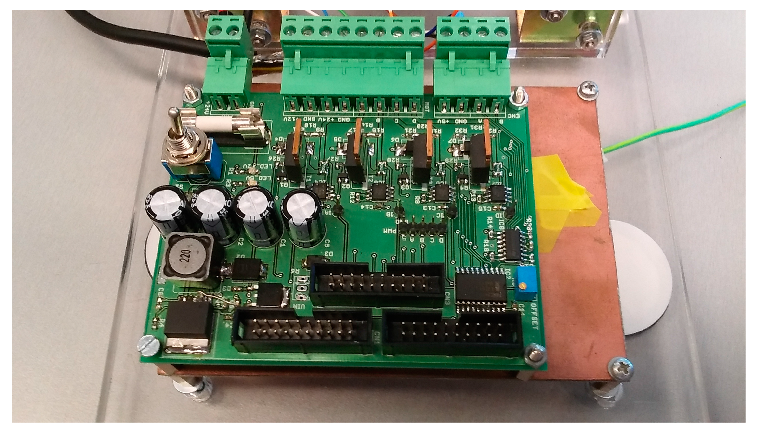
To demonstrate the effectiveness of the proposed approach a four-phase reluctance motor has been considered. The dynamic characteristics of the motor have been measured through a series of experiments. The driver printed circuit board (PCB) designed and built to conduct experiments is presented in Figure 1, while the motor driver configuration is shown in Figure 2. The PCB driver was connected to the computer via a data acquisition card (RT-DAC4/PCI, Inteco, Kraków, Poland). The data acquisition card provides a library to implement the I/O functions in the C language. The software to control the motor was, therefore, written in the C language. This allows the possibility to apply a custom waveform of motor voltages and measure the motor responses, like currents and position. The software was implemented with real-time priority, hence, it gives a sampling performance of 10 kHz.
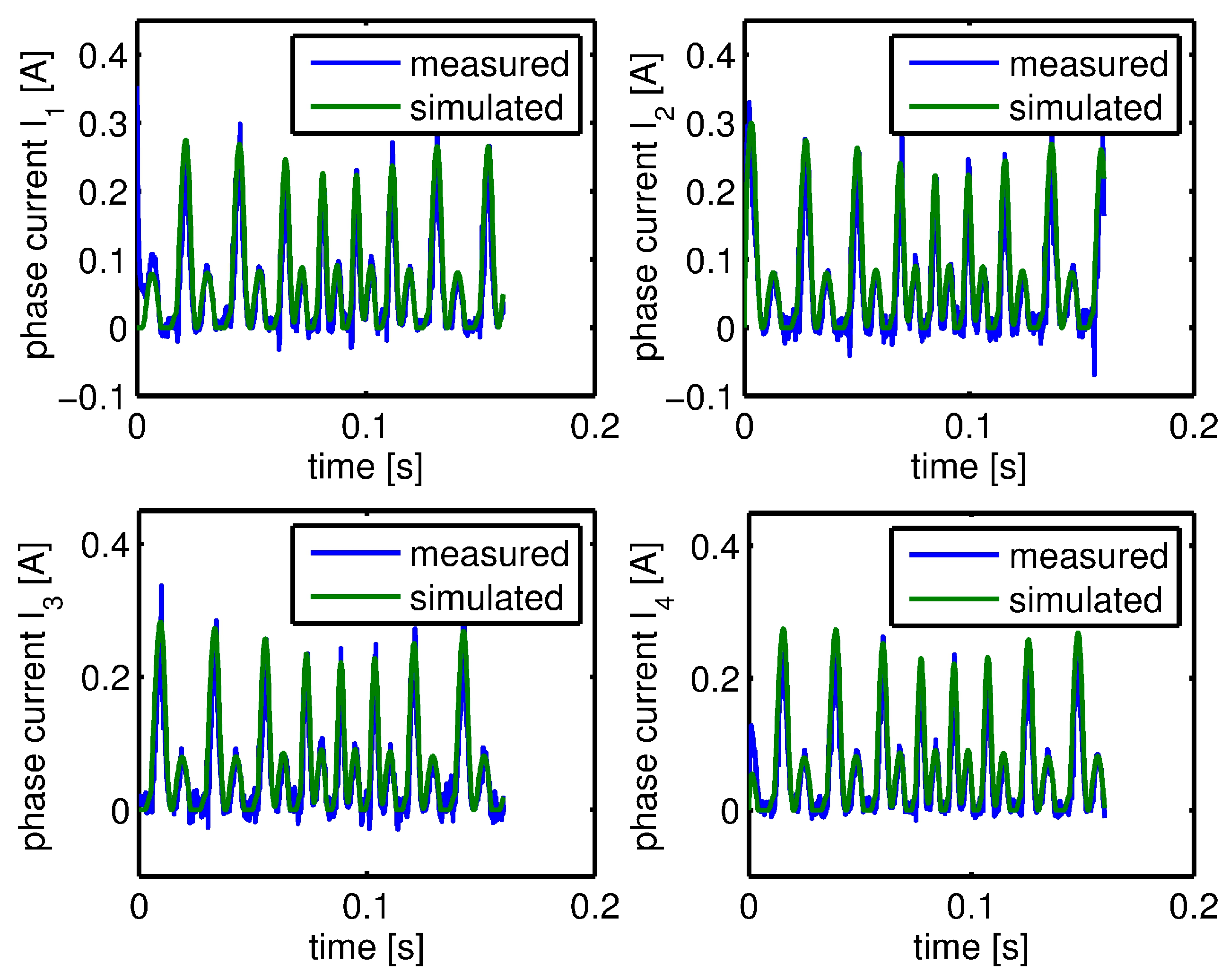
In the first stage of measurements the motor inductance waveform was found; the resultant inductance waveforms and are shown in Figure 3. The winding resistance was measured directly using an ohmmeter and found to be equal to 75 Ω. Relying on these measurements the dynamic model of the motor was built. To verify the quality of the modelling, the motor was excited by a single phase square-wave voltage with an amplitude 25 V, with other motor parameters listed in Table 1. The comparison of current transients obtained from simulation and measurements is provided in Figure 4, showing a very satisfying agreement.
9. The Optimization Process
The goal of this exercise was to find a current waveform which would provide a reference torque of . Furthermore, we considered a unipolar driver with constrained voltage between 0 and 25 V.
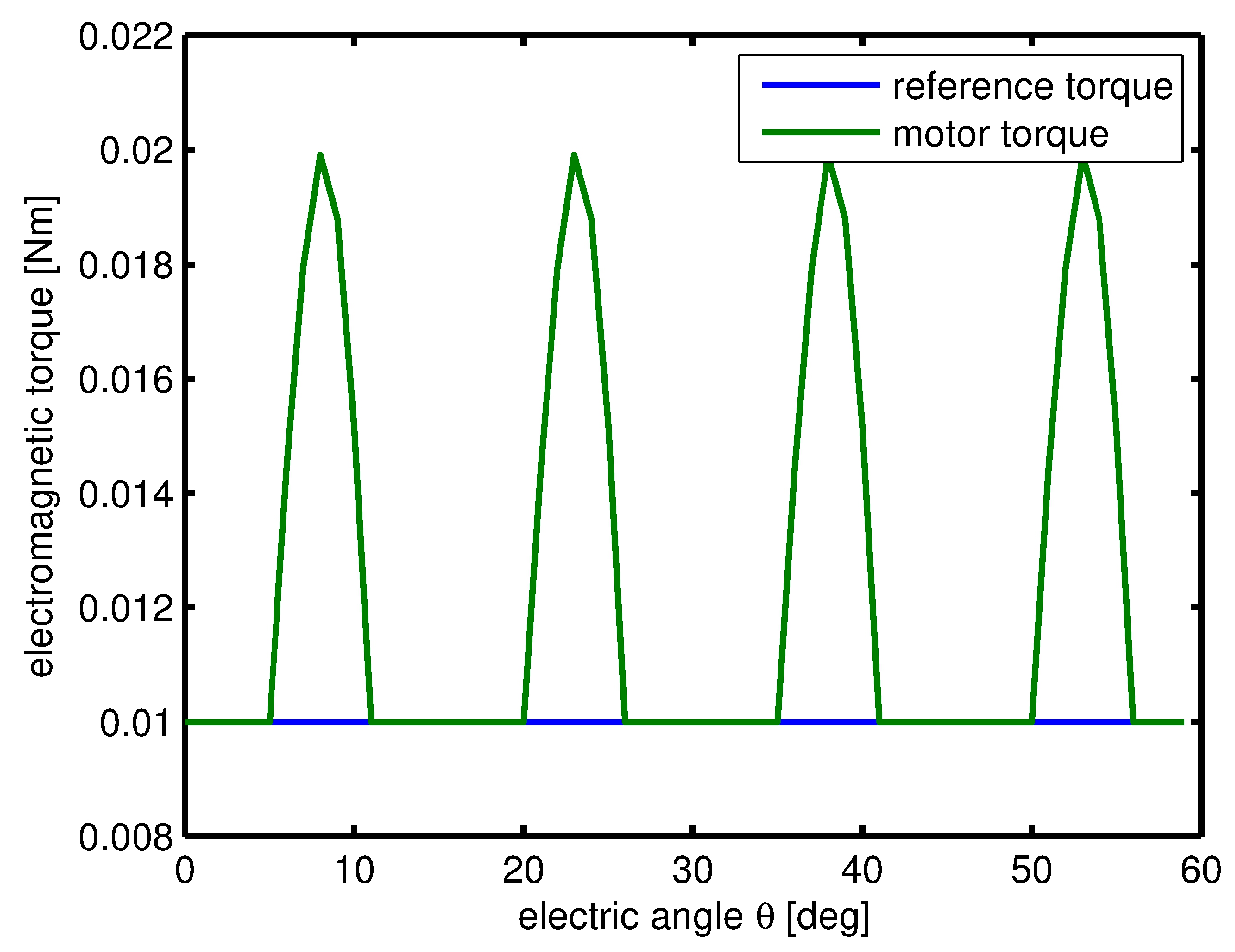
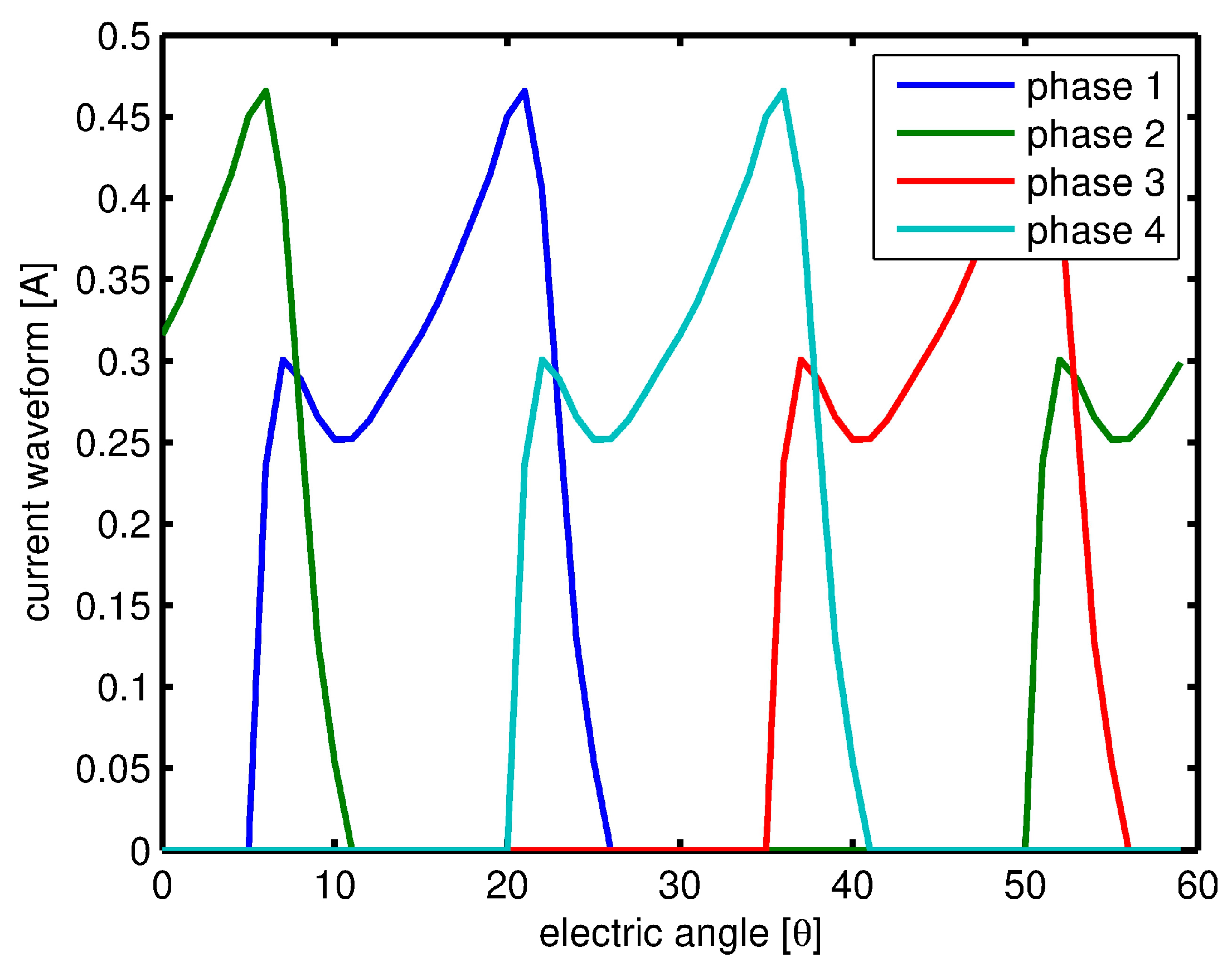
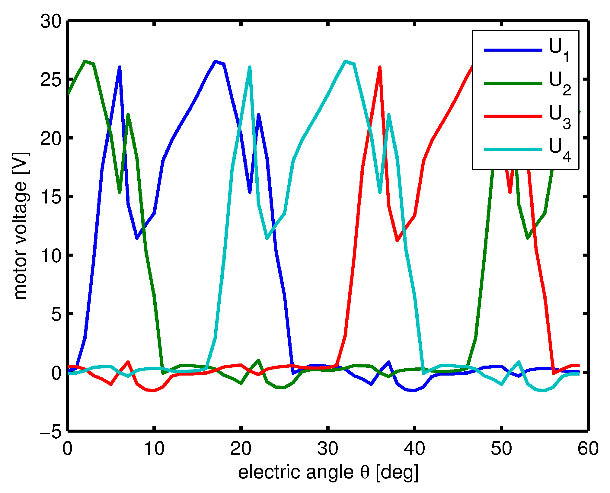
First, we found the current waveforms using the method proposed in [9]; this approach, however, does not account for mutual inductances and causes high levels of torque ripples in the electromagnetic torque, clearly visible in Figure 5. In this case the torque was found by considering an exponential torque shape function (TSF). Conversely, other types of TSF give similar results with high torque ripples because none of them consider mutual inductance. In Figure 6 and Figure 7 the current and voltage are shown resulting from the TSF method. Since voltage constraints have not been applied, the highest value is about 35 V and is above the upper limit.
We now follow the methodology described in previous sections, which is optimizing the performance according to Equation (33). We applied the square waveform current as an initial value for solving the optimisation problem. The weights were set to , , and . These values were chosen in order to achieve a good compromise between small torque error, constrained voltage, and the sensitivity of inductance.
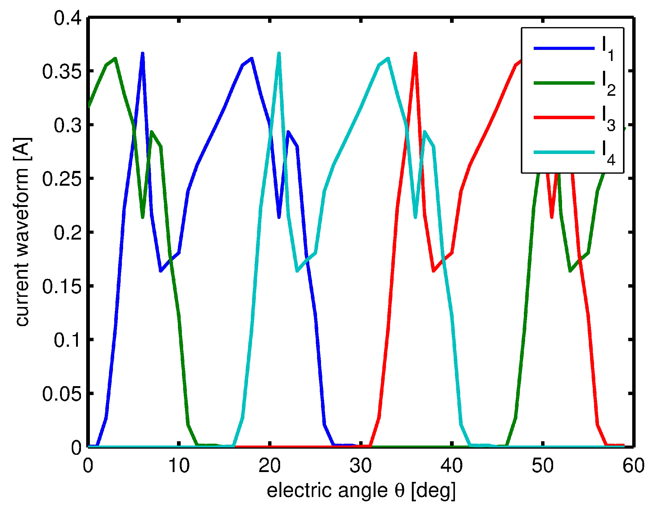
We used a gradient search algorithm as gradients were available. The optimization results are presented in Figure 8, Figure 9 and Figure 10, where the electromagnetic torque, current and voltage are shown. The torque ripples are below 2%, which is a very good result. We, therefore, conclude that the mutual inductance must be considered in these calculations. Furthermore, we have achieved the constrained voltage objective with limits from 0 V to 25 V.
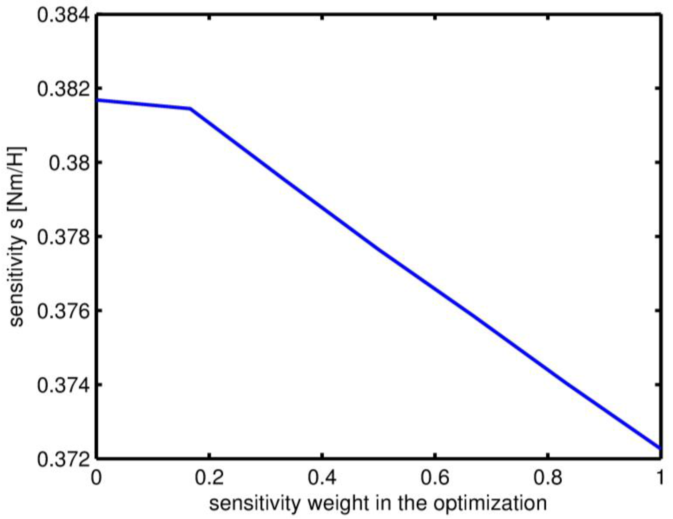
The next step is the analysis of the consequences of the increased robustness of the current waveform. The robustness is secured by minimizing the sensitivity with respect to changes to parameters. This is important because inductance is always found with some error and it is desirable to choose a shape which is more robust to parameter changes. In Figure 11 it is demonstrated that with an increase of the weight we may achieve a smaller sensitivity of the current waveform. However, the unwelcome consequence is an increase of torque ripples, as presented in Figure 12.
10. The Closed Loop Control Algorithm
To verify the proposed methodology we operated the motor relying on current waveforms designed in the previous section. Thus, the control rule was set up as:
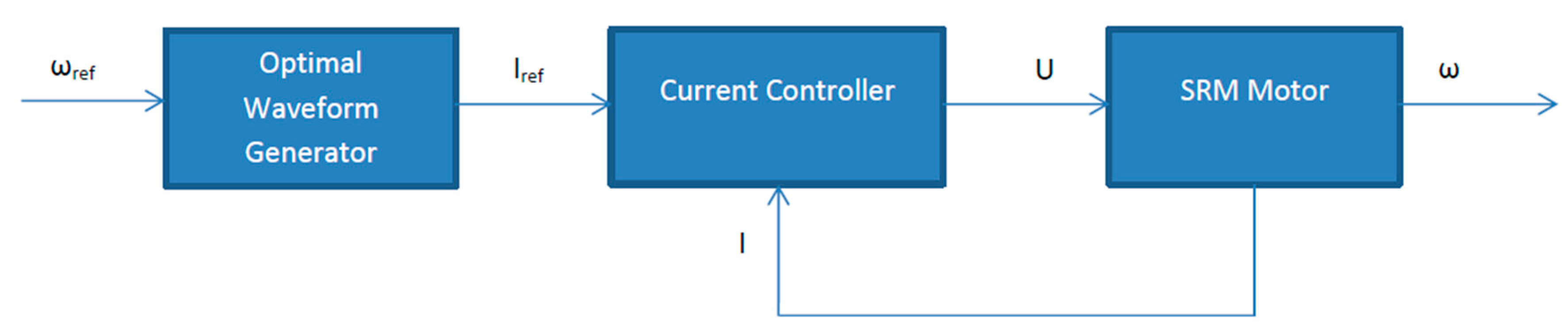
where is the input voltage vector, is the state current vector, are the self and mutual inductance matrices, and R is the resistance matrix. The feedback gain K was set to . The flowchart of the closed loop control system is presented in Figure 13.
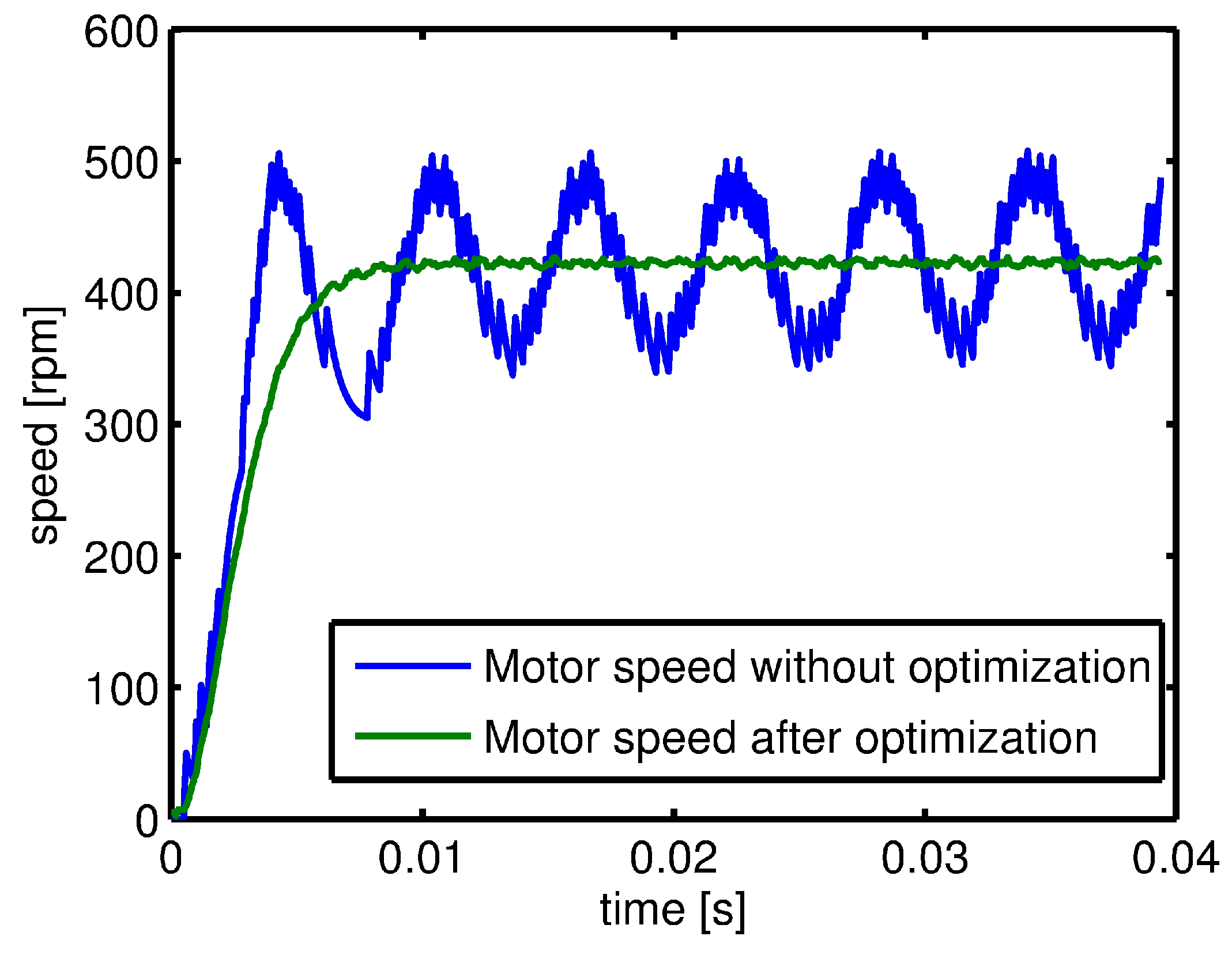
Next, we applied the selected control rule to run the motor with a constant speed of 400 rpm. The reference current waveform was generated by the optimization formulation defined in Equation (33) and solved in the previous section. The motor currents were driven using the control rule defined in Equation (34). Owing to the optimization of current waveforms, we achieved a reduction of the torque ripple. It can be seen in Figure 14 that speed ripples before optimization had an amplitude of 37.5%, while after optimization were reduced to 2.5%. This shows that the optimization improved significantly the quality of motion.
11. Conclusions
The paper proposes a novel methodology for determining current waveforms of switch reluctance motors. The approach is general and may be applied to different kinds of a reluctance motor, including three-phase, five-phase, and other types. The transformation from time to position domain facilitates accurate modelling of phase inductance. An optimisation formulation has been put forward which allows considerations of constrained voltage and sensitivity as a multi-objective problem combined with the reduction of torque ripples. The advantages of the proposed approach were demonstrated through simulations and verified experimentally.
Author Contributions
Jakub Bernat conducted the background research, defined the equations, implement the solver, and wrote the manuscript. Jan K. Sykulski directed the research, reviewed the manuscript, and proposed changes and improvements to its structure. Sławomir Stępień designed and conducted the simulations, experiments and analyzed the data.
Conflicts of Interest
The authors declare no conflict of interest.
References
- Vijayakumar, K.; Karthikeyan, R.; Paramasivam, S.; Arumugam, R.; Srinivas, K.N. Switched Reluctance Motor Modeling, Design, Simulation, and Analysis: A Comprehensive Review. IEEE Trans. Magn. 2008, 44, 4605–4617. [Google Scholar] [CrossRef]
- Stępień, S.; Bernat, J. Modeling and optimal control of variable reluctance stepper motor. COMPEL Int. J. Comput. Math. Electr. Electron. Eng. 2011, 30, 726–740. [Google Scholar] [CrossRef]
- Ilic-Spong, M.; Marino, R.; Peresada, S.M.; Taylor, D.G. Feedback linearizing control of switched reluctance motors. IEEE Trans. Autom. Control 1987, 32, 371–379. [Google Scholar] [CrossRef]
- Wallace, R.S.; Taylor, D.G. A balanced commutator for Switched Reluctance Motors to Reduce Torque Ripple. IEEE Trans. Power Electron. 1992, 7, 617–626. [Google Scholar] [CrossRef]
- Filicori, F.; Guarino, C.; Bianco, L.; Tonielli, A. Modeling and Control Strategies for a Variable Reluctance Direct-Drive Motor. IEEE Trans. Ind. Electron. 1993, 40, 105–115. [Google Scholar] [CrossRef]
- Buja, G.S.; Menis, R.; Valla, M.I. Variable Structure Control of an SRM Drive. IEEE Trans. Ind. Electron. 1993, 40, 56–63. [Google Scholar] [CrossRef]
- Illic-Spong, M.; Miller, T.J.E.; MacMinn, S.R.; Thorp, J.S. Instantaneous torque control of electric motor drives. IEEE Trans. Power Electron. 1987, 2, 55–61. [Google Scholar] [CrossRef]
- Xue, X.D.; Cheng, W.E.; Ho, S.L. Optimization and Evaluation of Torque-Sharing Functions for Torque Ripples Minimization in Switched Reluctance Motor Drives. IEEE Trans. Power Electron. 2009, 24, 2076–2090. [Google Scholar] [CrossRef]
- Moron, C.; Garcia, A.; Tremps, E.; Somolinos, J.A. Torque Control of Switched Reluctance Motors. IEEE Trans. Magn. 2012, 48, 1661–1664. [Google Scholar] [CrossRef]
- Cheok, A.D.; Fukuda, Y. A New Torque and Flux Control Method for Switched Reluctance Motor Drives. IEEE Trans. Power Electron. 2002, 17, 543–557. [Google Scholar] [CrossRef]
- Sahoo, S.K.; Dasgupta, S.; Panda, S.K.; Xu, J.X. A Lyapunov Function-Based Robust Direct Torque Controller for a Switched Reluctance Motor Drive System. IEEE Trans. Power Electron. 2012, 27, 555–564. [Google Scholar] [CrossRef]
- Bernat, J.; Kołota, J.; Stępień, S.; Sykulski, J. A steady state solver for modelling rotating electromechanical devices exploiting the transformation from time to position domain. Int. J. Numer. Model. Electron. Netw. Devices Fields 2014, 27, 213–228. [Google Scholar] [CrossRef]
Figure 1.
The motor driver electronic circuit.

Figure 2.
The motor phase windings and the unipolar drive circuit.
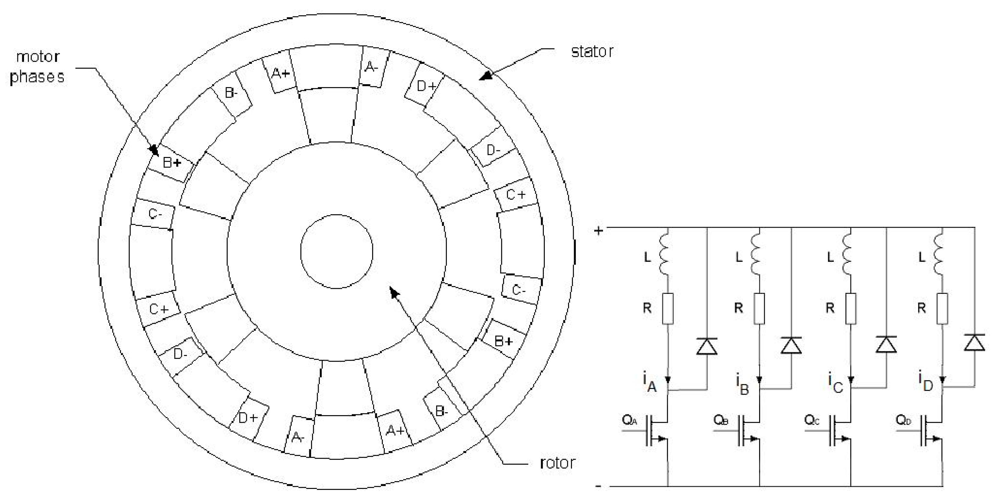
Figure 3.
The motor inductance waveforms for each phase.
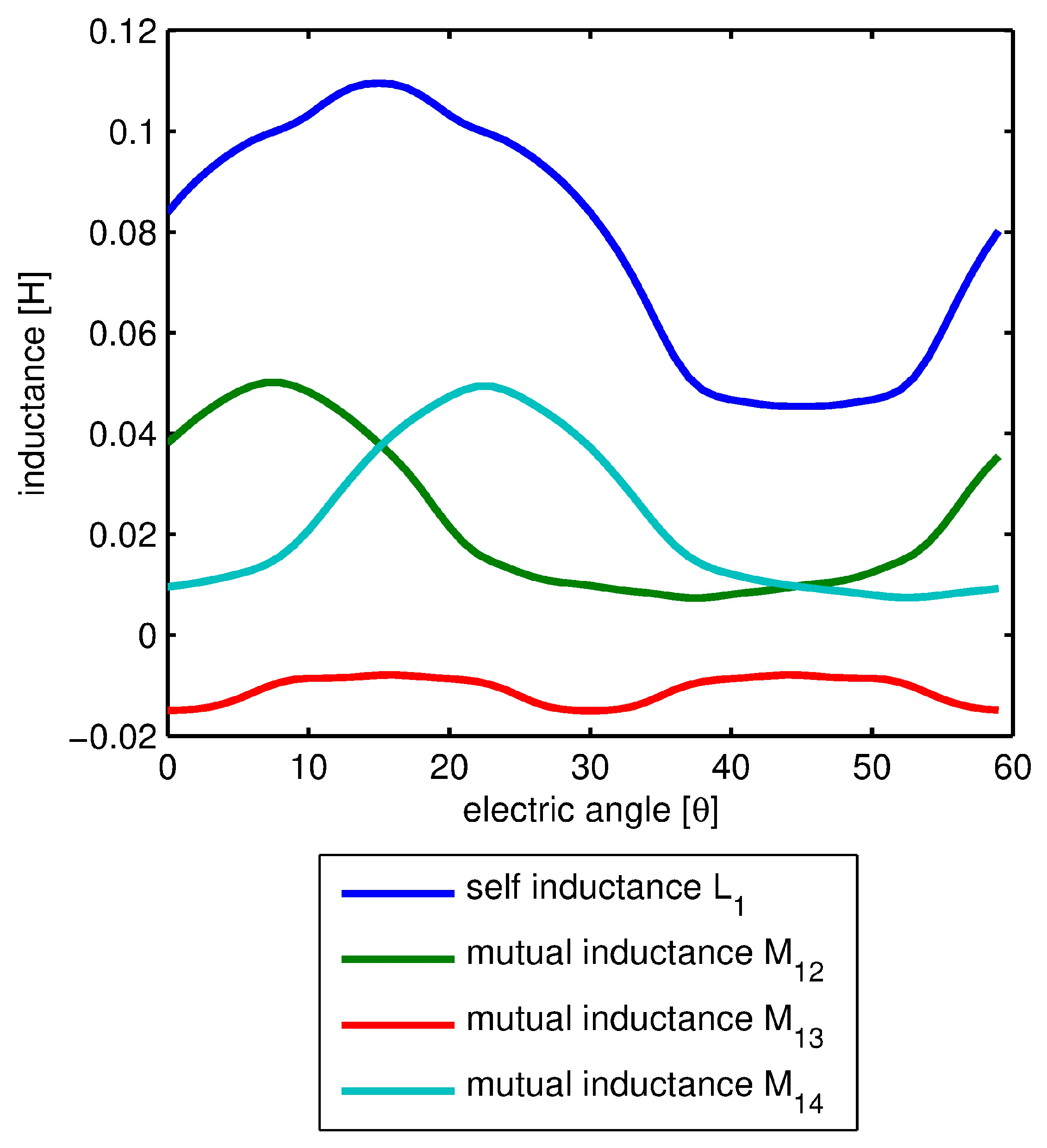
Figure 4.
The motor current waveforms for each phase.

Figure 5.
Torque waveform for the TSF method with an exponential waveform.

Figure 6.
Current waveform for the TSF method with an exponential current waveform.

Figure 7.
Voltage waveform for the TSF method with an exponential current waveform.
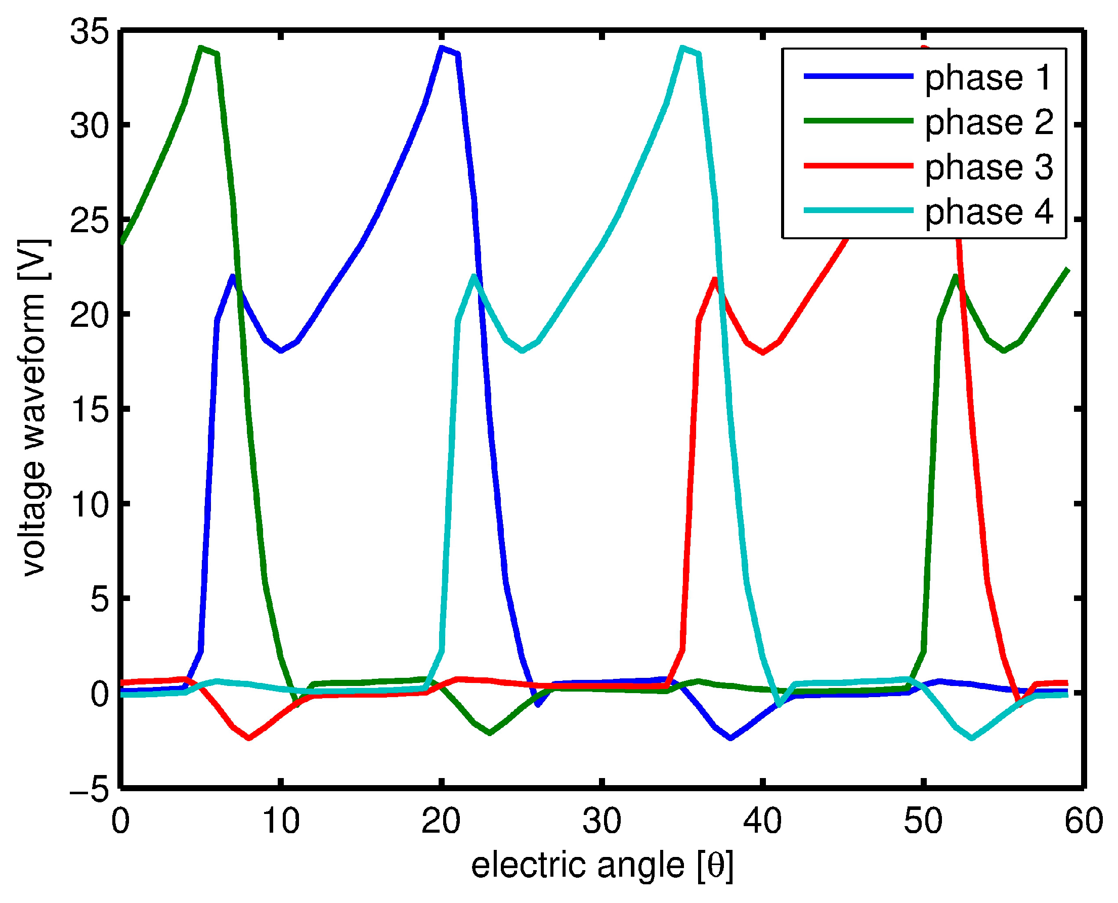
Figure 8.
Torque waveform found by optimization.
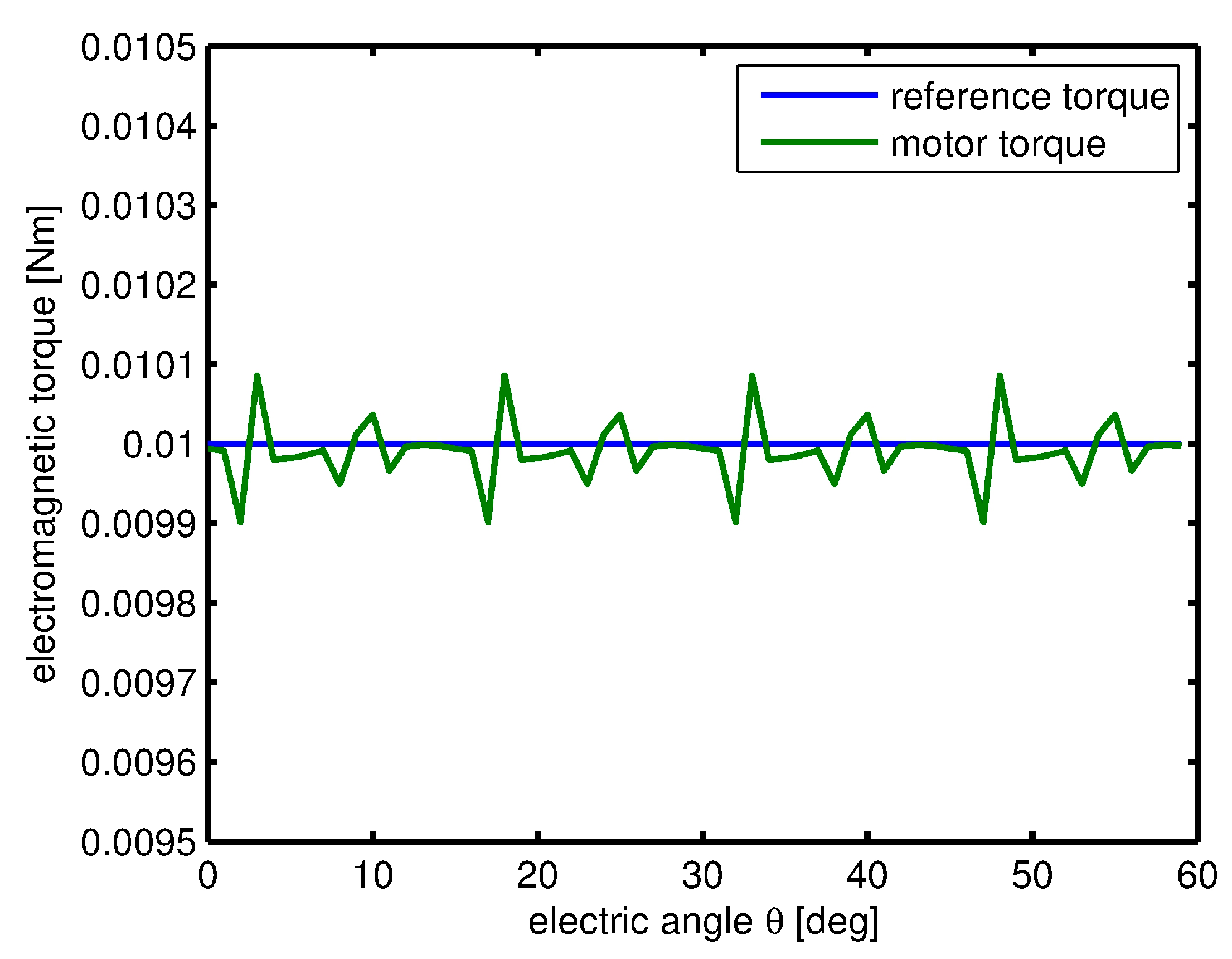
Figure 9.
Current waveform found by optimization with weights: , , and .

Figure 10.
Voltage waveform found by optimization with weights: , , and .

Figure 11.
Sensitivity value versus weight .

Figure 12.
Torque ripples versus weight .
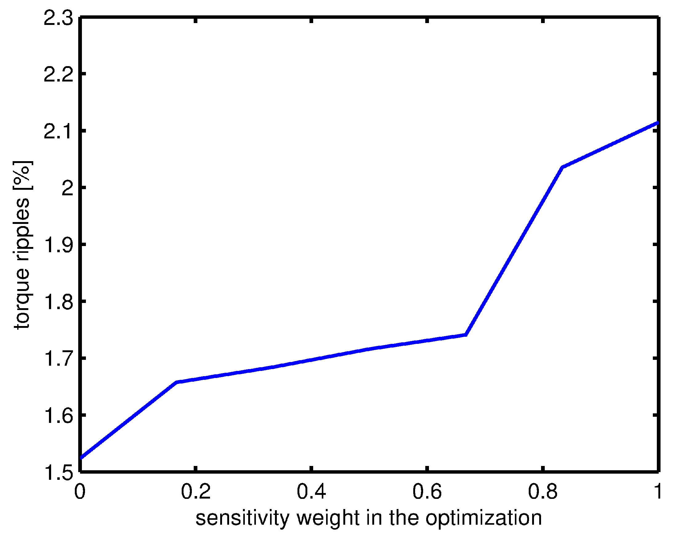
Figure 13.
Flowchart of the closed loop control system.

Figure 14.
Motor speed without and after optimization.

Table 1.
Motor parameters.
| Outer diameter of stator | 39 mm |
| Inter diameter of stator | 34 mm |
| Outer diameter of rotor | 26.96 mm |
| Inter diameter of rotor | 5 mm |
| Air gap length | 0.02 mm |
| Motor length | 30 mm |
| Resistance/phase | 75 Ω |
| Rotor inertia | 0.13 g∙cm2 |
© 2017 by the authors. Licensee MDPI, Basel, Switzerland. This article is an open access article distributed under the terms and conditions of the Creative Commons Attribution (CC BY) license (http://creativecommons.org/licenses/by/4.0/).
Share and Cite
MDPI and ACS Style
Bernat, J.; Stępień, S.; Sykulski, J.K. Determining Switched Reluctance Motor Current Waveforms Exploiting the Transformation from the Time to the Position Domain. Energies 2017, 10, 799. https://doi.org/10.3390/en10060799
AMA Style
Bernat J, Stępień S, Sykulski JK. Determining Switched Reluctance Motor Current Waveforms Exploiting the Transformation from the Time to the Position Domain. Energies. 2017; 10(6):799. https://doi.org/10.3390/en10060799
Chicago/Turabian StyleBernat, Jakub, Sławomir Stępień, and Jan K. Sykulski. 2017. "Determining Switched Reluctance Motor Current Waveforms Exploiting the Transformation from the Time to the Position Domain" Energies 10, no. 6: 799. https://doi.org/10.3390/en10060799
Note that from the first issue of 2016, this journal uses article numbers instead of page numbers. See further details here.