A New Methodology for Building-Up a Robust Model for Heliostat Field Flux Characterization

Abstract

The heliostat field of solar central receiver systems (SCRS) is formed by hundreds, even thousands, of working heliostats. Their adequate configuration and control define a currently active research line. For instance, automatic aiming methodologies of existing heliostat fields are being widely studied. In general, control techniques require a model of the system to be controlled in order to obtain an estimation of its states. However, this kind of information may not be available or may be hard to obtain for every plant to be studied. In this work, an innovative methodology for data-based analytical heliostat field characterization is proposed and described. It formalizes the way in which the behavior of a whole field can be derived from the study of its more descriptive parts. By successfully applying this procedure, the instantaneous behavior of a field could be expressed by a reduced set of expressions that can be seen as a field descriptor. It is not intended to replace real experimentation but to enhance researchers’ autonomy to build their own reliable and portable synthetic datasets at preliminary stages of their work. The methodology proposed in this paper is successfully applied to a virtual field. Only 30 heliostats out of 541 were studied to characterize the whole field. For the validation set, the average difference in power between the flux maps directly fitted from the measured information and the estimated ones is only of 0.67% (just 0.10946 kW/m² of root-mean-square error, on average, between them). According to these results, a consistent field descriptor can be built by applying the proposed methodology, which is hence ready for use.

1. Introduction

In one hour, more energy arrives to the Earth from the sun than all that is consumed by humanity in a year [1]. Effectively benefiting from this resource is a good way to overcome pollution problems and the increase in demand as commented in [2,3]. In this context, solar central receiver systems (SCRS) are power facilities of major interest for renewable and sustainable energy generation.

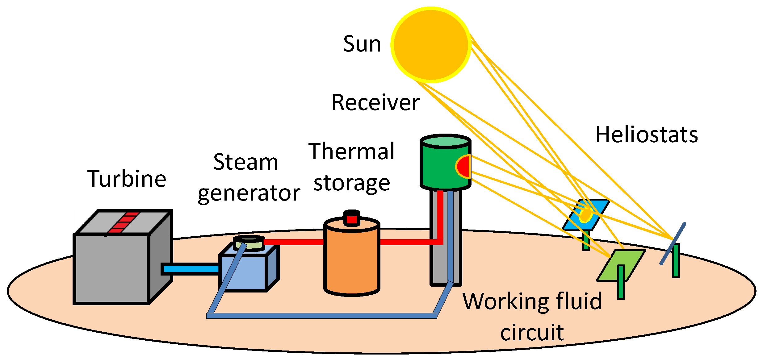
Considering the scope of this work, SCRS are formed by a radiation receiver, which is located in a tower, and a set of orientable high-reflectance mirrors called ”heliostats”. They track the apparent trajectory of the sun throughout the day to reflect and concentrate incident solar radiation on the receiver. This raw energy is then progressively transferred to a working fluid, which flows in its interior, and can be finally used in a turbine cycle to generate electricity. This kind of system features high thermodynamic efficiency [4,5] and power output stability based on thermal storage systems [4]. 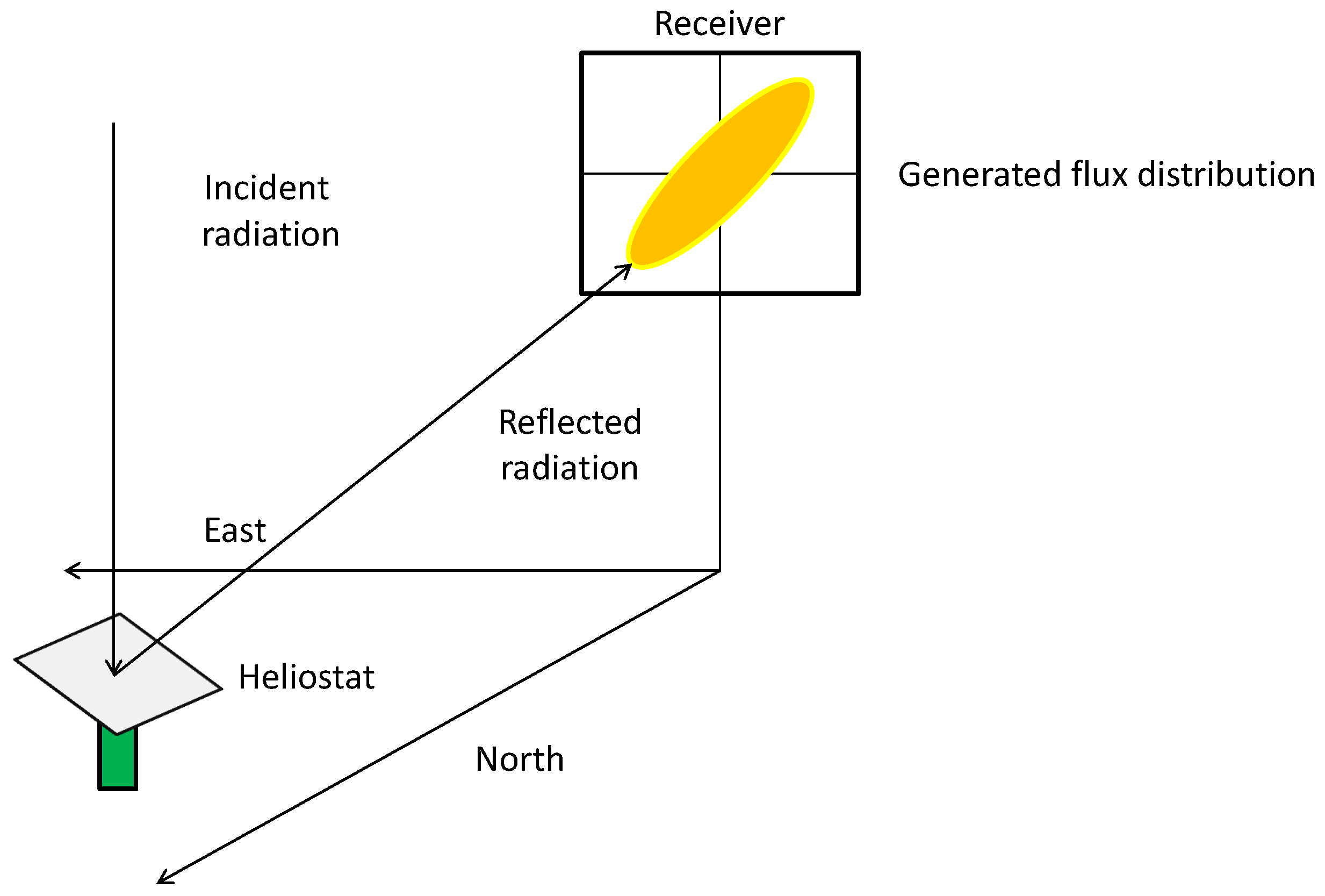Figure 1 shows a basic block diagram of an SCRS facility. Further information about SCRS can be found in [6], which is a popular online book whose 10th chapter is dedicated to this kind of systems. A more updated perspective in this topic can be obtained in [7], where current technologies of the most important parts of these facilities are nicely described. Similarly, Ref. [8] is a complete and updated review with valuable information and references. Finally, Ref. [9] is a good book focused on controlling techniques and also featuring a chapter dedicated to SCRS.

The flux distribution reflected by the set of heliostats over the receiver is a key aspect to consider when designing and controlling SCRS. Both operational efficiency and safety are directly linked to the achieved power distribution [10,11]. Thus, being able to simulate and characterize the behavior of heliostat fields is of major interest. In fact, there are numerous tools that can be used to simulate the flux distribution formed over the receiver by a certain heliostat field [12,13]. They can be classified into two main groups, detailed ray-tracing software, such as SolTrace [14] and Tonatiuh [15], and analytical approaches, such as those used by HFLCAL [16] and DELSOL [17]. Although ray-tracers are more precise and flexible for modeling complex situations, they are significantly more time-consuming than analytical models [10,11]. This is the main reason because they are preferred for field design optimization. In addition, they can also facilitate management of flux information just by working with the parameters linked to the selected model. This feature could be really appreciated when it is necessary to save flux information, as proposed in [18], especially from large fields.

In relation to flux map estimation at design, it is addressed by numerous works. In [19], an efficient model of a heliostat field is defined for its optimization. It is based on working with a discretization of the surface of heliostats and studying a simplified set of rays, which is successfully validated with SolTrace. Additionally, a promising distribution pattern is proposed. It is inspired from spiral patterns of the phyllotaxis disc and can reduce the surface of the field while also increasing its efficiency. In fact, that pattern has been later used in [20]. In that work, the HFLCAL model is used to compute the flux map of heliostats and estimate their interception losses. Additionally, an interesting proposal to reduce the computational cost of simulating and estimating the shading and blocking losses of the field is also made. It is a graphical method that limits those heliostats potentially blocking and shading a certain one to a sector in a circumference around it. In [5], a new field design strategy was proposed over the radial-staggered pattern. It is based on starting with a dense field in which all field losses apart from shading and blocking factors are reduced to progressively. Then, the field is progressively expanded to look for a trade-off between improving shading and blocking losses and the other factors. In [21], where this method is analyzed, detailed information of its underlying model is provided. Interesting comments about the flux map computation can also be found in that work comparing the HFLCAL approach to the method developed in [19]. In [22], the patterns of [5,19] are compared, and results show that both methods are equally capable of enhancing the performance of fields. In relation to their computational model, flux map estimation is based on the HFLCAL formulation. In [23], where patterns of [19] are compared to radial-staggering (similar to the strategy proposed in [5]), and the HFLCAL approach is also used to estimate the flux map distribution and interception losses. In that work, the pattern of [19] behaves better for north fields while the other one is more recommendable for surrounding and south fields and a hybrid solution is proposed. Finally, in [24], where design of multi-tower fields and receiver selection is addressed, HFLCAL is also used.

Regarding field characterization for control purposes, several recent papers are very interesting about that topic. In [11], their main goal is to obtain a homogeneous flux distribution with an acceptable spillage factor. A TABU search is applied to determine the best aim point of every heliostat from a combinatorial perspective. HFLCAL is used to estimate the flux map of their target field due to its reduced runtime but after being validated with SolTrace. In [10], defining the aim points to get a homogeneous flux shape is also the objective. An extended genetic algorithm to solve the optimization problem and HFLCAL is used to estimate the behavior of the studied field too. In contrast to the previous works, in [18], dangerous radiation peaks are avoided while maximizing the receiver power output. In addition, a way of affording the computational cost of detailed ray-tracing with tools like SolTrace is described. Specifically, it is based on moving that time-consuming parts to a preliminary stage. In [25], where a combination of the methods designed in [10,11] is developed, a similar proposal is made. However, in that case, the detailed output of a ray-tracer is systematically fitted to a an analytical model, a composition of bi-variant Gaussian forms, which is more adaptable than a circular-based Gaussian distribution (used by models such as HFLCAL).

In this work, an innovative methodology is proposed for instantaneous heliostat field characterization aimed at controlling support. Instead of being based on detailed ray-tracing or convolution analytical models, it defines a general procedure to merge the flexibility of an analytical representation with the precision of ray-tracers (or real data if available). To do so, the process benefits from the regularity of most fields and some statistical procedures to finally obtain an analytical field descriptor. The only really similar approach that has been found in the literature is applied in [25], where all the flux maps are iteratively fitted to an analytical model. In this work, an abstract generalization of that approach is formalized. Furthermore, instead of requiring access to the flux maps of the whole field, only the most descriptive subset is studied and fitted to any analytical expression selected. Then, the underlying behavior of the parameters observed at fitting is modeled. Upon success, a compact field descriptor or ”snapsho” of any studied field, at a certain instant, can be built. Therefore, the overall effort to generate, store and share the information of a field can be significantly reduced. It can also facilitate the generation of large synthetic flux map datasets for preliminary research in areas where this kind of information is needed, e.g., automatic control. Despite potential precision loss from real data, it is expected to consistently mimic the main behavior and trends of any field.

In order to prove the goodness of the proposed methodology, a field of several hundreds of heliostats has been virtually built as a test-bed. It has been designed according to the method described in [26], which avoids blocking. Hence, this phenomenon is not covered in the example. However, as detailed later, there are no limits to implicitly cover it or any other loss factor affecting flux maps. The rest of the paper is organized as follows: in Section 2, the methodology is abstractly described. Then, in Section 3, a sample test case is shown in detail. Finally, in Section 4, conclusions are drawn and future work is exposed.

2. Methodology Description

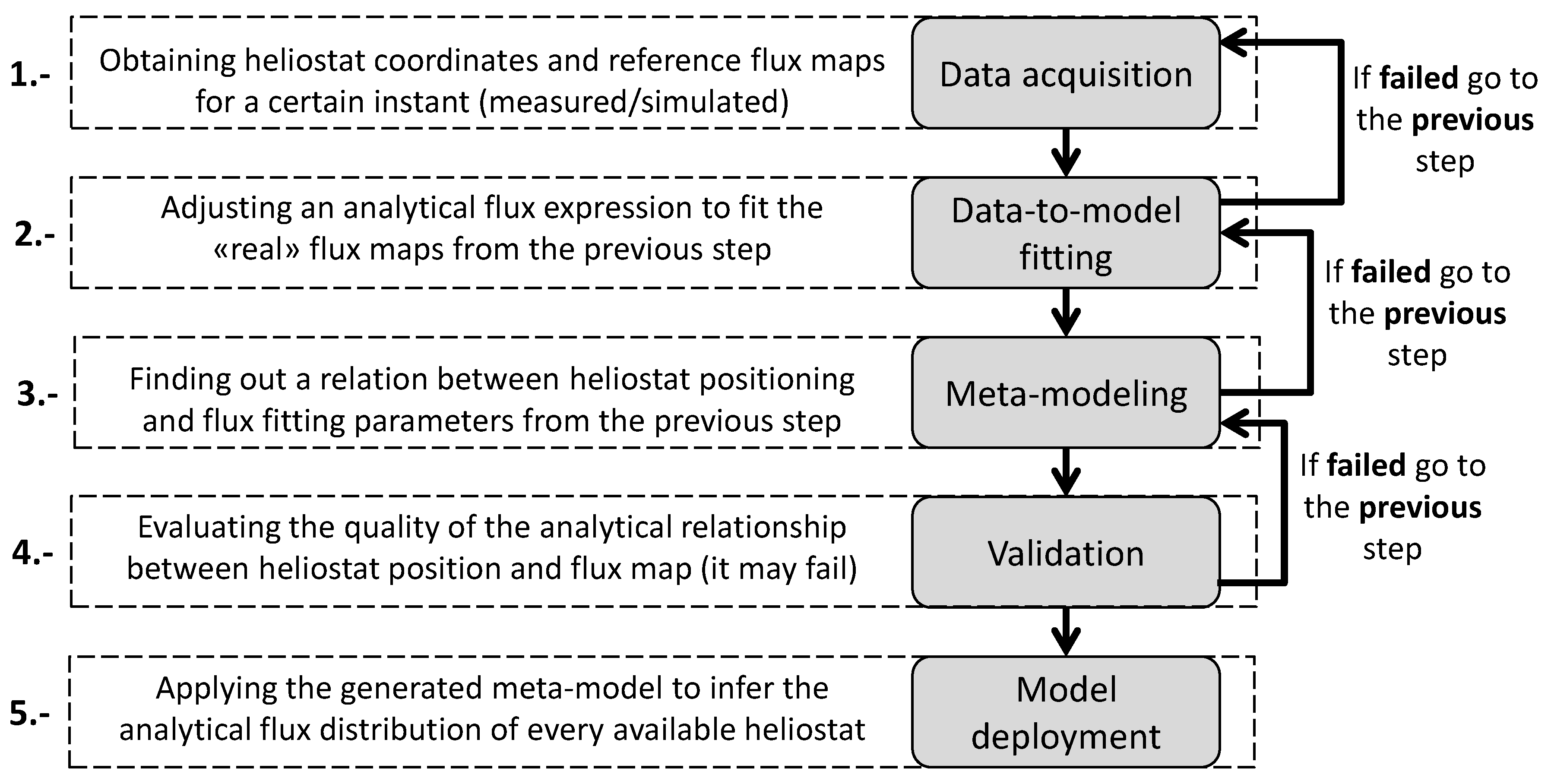
The main idea of the proposed methodology is to study in depth a descriptive subset of heliostats. Then, their behavior is linked to a common expression whose parameters are modeled to characterize the whole field at a desired operational state. Hence, it makes it possible to finally estimate the flux distribution of any heliostat depending on its position. Specifically, the methodology defines five consecutive steps: (i) data acquisition; (ii) data-to-model fitting; (iii) meta-modeling; (iv) validation and (v) model deployment. A complementary scheme of the procedure is shown in Figure 2.

2.1. Data Acquisition (DA)

In order to apply the methodology, it is necessary to know: (i) the physical properties of the field and (ii) the flux maps of a descriptive subset of heliostats. The whole procedure is based on the information collected at this stage.

In relation to the physical details of the target field, the minimum information required is the position of its descriptive heliostats, i.e., all zones should be covered. Otherwise, it would not be possible to correlate the position of every heliostat with its flux distribution. Let us denote I as the information set which defines the position of any heliostat h. It can be structured as a table formed by $\iota$ columns and H rows, where $\iota$ and H are the numbers of descriptive fields and known heliostats, respectively. Hence, a certain heliostat, h, is identified by a particular row $I_h=(I_{1_h},\cdots ,I_{{\iota }_h})$ in which every component is of a different type of positioning information. For instance, $I_{1_h}$ and $I_{2_h}$ could be the polar coordinates of heliostat h while $I_{3_h}$ and $I_{4_h}$ could be the Cartesian ones. In fact, as later steps require filtering and/or combining the available positioning data, it is convenient to provide redundant information at the beginning.

Regarding the reference flux maps, those generated by a known subset of H heliostats, S, at the target instant, are required. Flux maps, which can be seen as ”pictures”, are matrices that describe how the radiation density reflected by every heliostat is distributed over the receiver. Considering that the field is configured depending on the position of the sun, the obtained maps define the instantaneous component of the methodology. Hence, the same field would be characterized for a certain instant of time $t_0$ or $t_1$ depending on them. In this context, the flux map of a certain heliostat $h\in S$ will be denoted as $F_h$. Heliostats in S should cover all zones in the field to be descriptive in later modeling steps. S should also be large enough to be divided into a modeling subset and a validation one when required. Additionally, it must be highlighted that properties of the maps at acquisition should be inherited by the resulting characterization. Thus, if an appropriate sample of maps is gathered, energy losses such as blocking and shading could also be implicitly estimated. However, later steps can become significantly more difficult to fulfill and a trade-off between complexity and final requirements must be found.

Finally, it is important to note that the methodology does not define any source from which to get the flux maps. Consequently, input information could be achieved either from real measurements and/or simulation (e.g., SolTrace or Tonatiuh) and the same method is compatible with both real and virtual fields. Furthermore, even with real fields, it could be useful to complement measured and simulated information because simulators enhance flexibility of acquisition conditions. For instance, larger virtual receivers can be used to grant complete flux maps without spillage.

2.2. Data-to-Model Fitting (DF)

On success, the proposed methodology should allow for adapting the parameters of a common analytical expression to describe the flux maps linked to any heliostat of the field. Thus, at this step, it is necessary to define a base expression to model the flux distribution of heliostats. There are different analytical models to describe the flux distribution generated by heliostats. For instance, HFLCAL, which is based on a circular Gaussian distribution, is quite popular for this purpose and it has been successfully used in [10,11]. However, any parameter-based function could be selected for this purpose and a trade-off between resolution and complexity should be found: a function that is too simple might be inaccurate but an excessively complex one perhaps cannot be correctly fitted. The selected expression will be denoted as $F^{*}$ and its $\delta$ adjustable parameters as set D.

After selecting $F^{*}$, a certain tuple of parameters $D_h=(D_{1_h},\cdots ,D_{{\delta }_h})$ must be found for every heliostat $h\in S$ to be able to ”reproduce” its registered flux map, $F_h$. Obtaining the tuple $D_h$ that makes $F_{<D_h>}^{*}\approx F_h$ leads to facing a curve fitting problem whose resolution is not covered by the proposed methodology. However, from a practical point of view, the ”curve fitting toolbox” (CFT) for Matlab [27] is an interesting tool to do so. If there were problems to complete this step, different fitting methods should be explored. In case no good solutions can be found, it would be necessary to improve the information gathered and/or alter the acquisition conditions at ”DA” (as shown in Figure 2 by the arrow). For instance, if ray-tracing had been used, simulations could be run with more rays and a larger receiver.

The natural representation of the information obtained at this step is a table, T, which groups both positioning and analytical flux adjustment parameters. Every row of T is referred to a certain heliostat $h\in S$ and it is expected to have $\iota +\delta$ columns as depicted in Figure 3. Additional details included in it will be commented on later.

2.3. Meta-Modeling (MM)

This step aims to build a ”model for the flux model expression configuration”, i.e., a ”meta-model”, M, formed by $\delta$ internal models. To do so, the set of parameters, $D_h$, must be decomposed and studied. Hence, each column $t\in T$ defines the whole dataset to model parameter $D_t$ of $F^{*}$ in relation to the available positioning information. However, before trying to find a general application $I\to D_t$ for every parameter t, S should be divided into two disjoint subsets of heliostats, $S_M$ and $S_V$, which satisfy that $S_M\cup S_V=S$. While $S_M$ will be used for modeling, $S_V$ will be left for validation and the parameters of its heliostats must not be included to build the meta-model, M. This idea is depicted in Figure 3, where ”Heliostat 1”, as it is in $S_V$, is not used for modeling $D_1$.

At this step, I can be filtered to find its most descriptive components while also including additional processing operations. For instance, instead of using the $east$ coordinate of heliostats to model parameter t, i.e., building $M_t$, it might be better to use $abs\left(east\right)$ for a field featuring east/west symmetry. This idea is depicted in Figure 3, where $D_1$ is modeled from $I_1$ and $I_{\iota }$. Although specific resolution approaches are not covered, CFT could also be valid for this stage. If there were problems to complete modeling with different methods [28,29], some heliostats from $S_V$ can be moved to $S_M$. In case modeling still failed, it might be necessary to return to ”DF”. In fact, it could even be required to re-start from ”DA” by including more heliostats to S and/or expanding I. In the worst scenario, this approach could lead to including the whole field to look for a final meta-model.

This is the most important step of the proposed methodology. Upon success, a meta-model formed by a set of equations to generally estimate each parameter in D for every heliostat, linked to $F^{*}$, should be obtained. Hence, neither more detailed data nor curve fitting would be further needed: the field would have been characterized, for the target solar position, by only processing the information of a reduced set of heliostats. Otherwise, a compact field characterization would not be possible.

2.4. Validation (V)

This step proposes an explicit overall validation of the results achieved before being able to use the meta-model, M. However, there are no restrictions to include internal validation stages at previous steps. In fact, depending on the selected methods, they might include some kind of validation or, at least, quality metrics.

In general terms, ultimate validation requirements must be decided by the user. However, taking into account the context defined, two validation strategies can be considered. First, as the flux maps of all heliostats in S should be fitted to $F^{*}$ at ”DF”, the parameters predicted by M for those in $S_V$ can be numerically compared to the values obtained by the fitting method. Second, the reference flux maps gathered at ”DA” of those heliostats left in $S_V$ could be compared to their synthetic equivalent generated from M and $F^{*}$. Although both approaches can be combined for a more robust validation, the second one is most important as it is based on comparing the reference maps with the analytically predicted ones.

Validation, by definition, is oriented at analyzing $S_V$. However, if the user needed a complete performance perspective, the previous procedures could be applied to the whole set S. Even though those heliostats in $S_M$ should not be taken into account to validate M, the proposed criteria could help to identify important differences in its behavior between heliostats in $S_M$ and $S_V$.

2.5. Model Deployment (MD)

At this point, M should be suitable for computing the configuration parameters, $D_h$, related to $F^{*}$, for any heliostat in the field (not only for those in S). Thus, the flux distribution map of every heliostat can be synthetically estimated on demand for the initial acquisition conditions (e.g., solar position, inherited properties, etc.).

From now, the field flux maps can either be inflated from the analytical expression and stored or parametrically saved with a negligible cost. The first option may reduce further computational time, while the second one requires an extra inflating step but the final precision of the maps can be adjusted. Decision depends on the context in which heliostat field characterization was needed.

3. Application Example

3.1. Field Design

Before applying the proposed methodology, it is necessary to have a target field. The definition of the selected one will be explained in this subsection. In fact, it does not exist in reality and has been ad hoc defined to show how a researcher could autonomously design and characterize a sample testing field. It is assumed to be in the south of Spain, at ${37}^{\circ }{5}^{\prime }$ N, $2^{\circ }{21}^{\prime }$ W, and has 541 heliostats over a flat surface. The field will be virtually built with the open-source ray-tracer Tonatiuh [15].

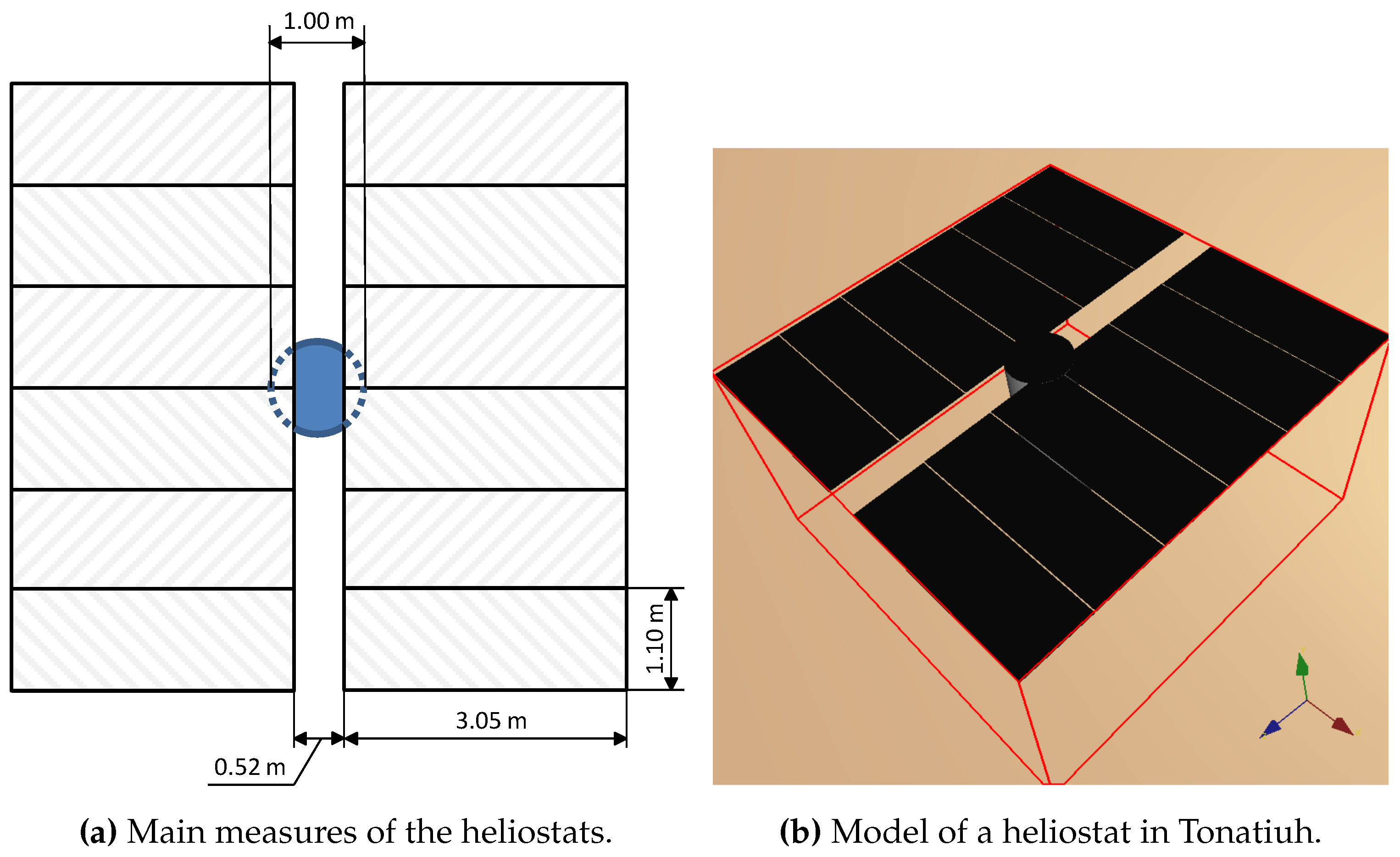
The heliostat model aims to be a clone of the one deployed in the CESA-I [30] field, which is approximately in the same location. It consists of 12 curved reflecting facets that are divided into two equal columns and mounted on a supporting ”T” structure. There is a distance of $0.516$ m between the two columns. Every facet has a curvature radius of 350 m, a width of $3.05$ m and a height of $1.1$ m. The central bar of the supporting structure has a vertical length of $3.65$ m and $0.5$ m of radius.

In Figure 4a, a schematic diagram of the heliostat model is shown. Canting of facets is adjusted on axis to the slant range. For instance, heliostats in the first row have a focal length of $216.6$ m (the module of a vector pointing from their center to the receiver). Optical error linked to every heliostat has been randomly generated in the range $[1.4,2.0]$ mrad according to records from the CESA-I field. Heliostats aims at a $10\times 10$ m² flat-plate receiver, which is due north and parallel to the west–east plane. Its center is at 155 m over the ground and it is mounted on a cylindrical structure that has a radius of 10 m and a height of 165 m.

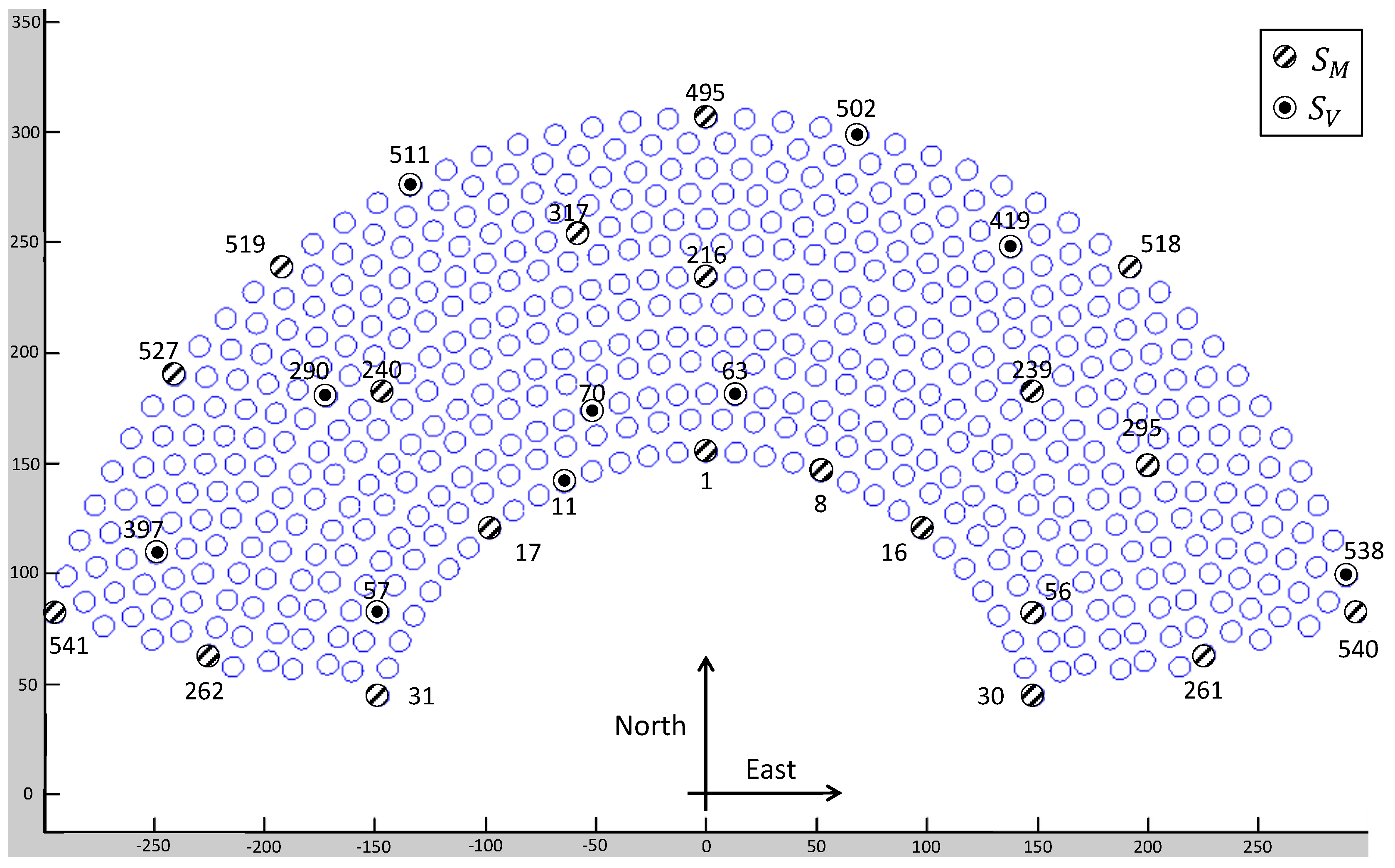
Heliostats follow the pattern described in [26] and form the symmetric north-field shown in Figure 5. No special field type is explicitly required by the methodology, though. The parameters given to the algorithm described in [26] to generate the field are listed in

Table 1. Parameters given to the layout generation algorithm described in [26].

Parameter Value	Description
$l_m=6.600$ m	Length of the reflective surface of heliostats (see Figure 4a)
$w_m=6.616$ m	Width of the reflective surface of heliostats (see Figure 4a)
$z_0=3.650$ m	Height of the heliostat center from the base.
$f_a=0.922$	Ratio of the reflecting and total surface of a heliostat.
$dS=0.000$	Extra separation distance.
$l_r=10.000$ m	Receiver vertical height.
$H_t=155.000$ m	Aim point height (receiver center).
${\beta }_L=0^{\circ }$	Terrain slope rising from the tower.
${\psi }_{max}=1.309$ rad	Maximum angular direction.
$R_{max}=300.000$ m	Maximum ring radius.

.

3.2. Data Acquisition (DA)

First, as the target field has been designed for this work, positioning data is directly available for all heliostats. Thus, the information set I is implicitly defined and accessible. Second, the instantaneous flux maps of a selected set of heliostats, S, are required for analysis. Specifically, the characterized instant assumes a solar altitude and azimuth of $72.{74}^{\circ }$ and ${180}^{\circ }$, respectively. This is the estimated solar position on the 21st of May at noon in the facility location [6].

Regarding S, heliostats at extreme west, east, north and intermediate positions will be selected. By proceeding this way, all extreme and mid-point positions should be covered. In Figure 5, the final heliostat selection can be seen (their tag can be ignored for now). In

Table 2. Positioning details of the heliostats in S.

ID	East (m)	North (m)	Radius (m)	Azim. (rad)
1	0.0000	155.0000	155.0000	0.0000
8	51.9054	146.0508	155.0000	0.3415
11	−64.1693	141.0933	155.0000	−0.4268
16	97.8171	120.2365	155.0000	0.6829
17	−97.8171	120.2365	155.0000	−0.6829
30	148.5154	44.3642	155.0000	1.2805
31	−148.5154	44.3642	155.0000	−1.2805
56	148.5815	81.8856	169.6517	1.0613
57	−148.5815	81.8856	169.6517	−1.0613
63	13.2202	180.6278	181.1110	0.0731
70	−52.1778	173.4320	181.1110	−0.2922
216	0.0000	234.1500	234.1500	0.0000
239	146.8911	182.3438	234.1500	0.6781
240	−146.8911	182.3438	234.1500	−0.6781
261	225.6014	62.6917	234.1500	1.2997
262	−225.6014	62.6917	234.1500	−1.2997
290	−171.9597	179.8783	248.8500	−0.7629
295	199.8437	148.2862	248.8500	0.9324
317	−58.3413	253.6872	260.3092	−0.2260
397	−248.9920	108.9087	271.7685	−1.1585
419	137.9184	247.3792	283.2277	0.5086
495	0.0000	306.1462	306.1462	0.0000
502	68.6144	298.3581	306.1462	0.2260
511	−133.7379	275.3901	306.1462	−0.4521
518	192.0570	238.4106	306.1462	0.6781
519	−192.0570	238.4106	306.1462	−0.6781
527	−240.6045	189.3013	306.1462	−0.9042
538	289.8686	98.4973	306.1462	1.2432
540	294.9690	81.9681	306.1462	1.2997
541	−294.9690	81.9681	306.1462	−1.2997

, the positioning information of heliostats in S is included. The first column contains the identification number of every heliostat. The second and third columns correspond to the 2D Cartesian coordinates of every heliostat over the field. In addition, as introduced, some redundant information can be useful at later steps. Hence, the fourth and fifth columns contain their polar coordinates (where North and East are at $0^{\circ }$ and ${90}^{\circ }$, respectively). The colored rows correspond to the heliostats that will be assigned to $S_V$ for validation, but this information is not relevant for now. Table 2 can be seen as the non-abstract equivalence of the I part depicted in Figure 3.

Exclusive simulations have been launched in Tonatiuh, with every heliostat aimed at the receiver center, in order to get the corresponding flux maps at the instant of interest. Thus, shadowing and blocking phenomena have not been taken into account (the layout generation method used aims to avoid blocking, though). A Pillbox Sun-shape distribution has been used with 1 kW/m² of flux density and 10 million rays. Heliostats in the most extreme positions required, however, 20 million rays and a $20\times 20$ receiver to get adequate maps. The collision maps generated by Tonatiuh have been then loaded in Matlab to build the final flux density ”pictures” of every heliostat as histograms. A discrete grid formed by cells of $0.04\times 0.04$ m² over the receiver surface has been used to do so.

3.3. Data-to-Model Fitting (DF)

In this example, a bi-variant or elliptic-based Gaussian distribution will be used to describe the flux maps generated by heliostats. This decision is based on the fact that, in contrast to circular-based Gaussian distribution, a bi-variant one can directly handle elliptic-based forms. Hence, as highlighted in [25], more adaptable flux maps can be obtained.

In Equation (1), the bi-variant Gaussian distribution used as $F^{*}$ is formulated. x and y are the coordinates on the receiver plane defined along its X and Y dimensions, respectively. P is the power contribution of heliostat h (in kW), $\rho$ is the correlation between x and y, ${\sigma }_x$ and ${\sigma }_y$ are the standard deviation along X and Y, respectively (in meters). Finally, ${\mu }_x$ and ${\mu }_y$, the mean in a Gaussian probability function, define the central point of the flux distribution, i.e., the aiming point of heliostat h. P, $\rho$, ${\sigma }_x$ and ${\sigma }_y$, as they define the general shape of the flux distribution, form the parameter set D. However, ${\mu }_x$ and ${\mu }_y$ have not been included in that set because the aim point of all heliostats, which was fixed as the receiver center at acquisition, is not expected to significantly alter the shape of flux maps. Thus, the flux map of every heliostat will be estimated on any point of the receiver by simply varying ${\mu }_x$ and ${\mu }_y$ from 0, i.e., the receiver center. This strategy, which is interesting in order to study aiming strategies, is viable considering that, for large distances between the heliostats and a normal-sized receiver, the map generated remains almost unaltered with independence of their aim point:

$$F_{<D_h>}^{*}(x,y)=\frac{P}{2\pi {\sigma }_x{\sigma }_y\sqrt{1-{\rho }^2}}{e}^{\left(-\frac{1}{2(1-{\rho }^2)}\left(\frac{{(x-{\mu }_x)}^2}{{\sigma }_x^2}+\frac{{(y-{\mu }_y)}^2}{{\sigma }_y^2}-\frac{2\rho (x-{\mu }_x)(y-{\mu }_y)}{{\sigma }_x{\sigma }_y}\right)\right)}.$$

(1)

Once the analytical model $F^{*}$ has been selected, the $\delta$ parameters of every heliostat $h\in S$ must be computed by fitting their flux maps, those acquired at the previous step, to $F^{*}$. To do so, as suggested in Section 2, the CFT tool has been used. It has been configured to use the ”Non-linear Least Squares” method with the algorithm ”Trust-Region” and the mode ”Least Absolute Residual”for robustness. Flux maps have been normalized according to the total summation of their representing matrix. The allowed real ranges for every member of D, adjusted after preliminary experimentation, are summarized next: $P\in \left[0.0,1.0\right]$, $\rho \in \left[-1.0,1.0\right]$, ${\sigma }_x\in \left[0.5,4.5\right]$ and ${\sigma }_y\in \left[0.5,4.5\right]$.

In

Table 3. Fitted parameters byCFT for the flux map of every heliostat in S.

ID	P (kW)	$\mathit{\rho }$	${\mathit{\sigma }}_{\mathit{x}}$ (m)	${\mathit{\sigma }}_{\mathit{y}}$ (m)
1	38.6405	−0.0003	0.6882	0.9544
8	38.5309	−0.2361	0.7316	0.9796
11	38.3254	0.2963	0.7636	1.0080
16	38.0629	−0.4815	0.8919	1.1070
17	37.6772	0.4878	0.8967	1.1110
30	36.7080	−0.9166	2.4170	2.4680
31	36.5241	0.9173	2.4200	2.4680
56	37.1653	−0.7438	1.5240	1.5190
57	36.9884	0.7693	1.5340	1.5330
63	37.9394	−0.0454	0.7768	0.9792
70	37.5858	0.1818	0.8235	1.0160
216	36.5834	−0.0003	0.9733	1.0850
239	36.5207	−0.3977	1.2410	1.1730
240	36.4163	0.3857	1.2080	1.1370
261	34.4667	−0.8848	3.3970	2.3070
262	34.8540	0.8925	3.4740	2.3600
290	35.8689	0.4258	1.3990	1.2260
295	35.6353	−0.5606	1.6650	1.3140
317	36.4444	0.1069	1.0800	1.1070
397	34.9722	0.7552	2.7380	1.7570
419	35.9613	−0.2371	1.2990	1.1920
495	35.7205	0.0016	1.2280	1.1970
502	37.4073	−0.0847	1.3050	1.2500
511	35.5648	0.1899	1.3870	1.2550
518	35.1758	−0.3307	1.5680	1.2650
519	35.0714	0.3192	1.5950	1.3020
527	34.8433	0.4765	2.0050	1.4030
538	33.7058	−0.7969	3.7820	2.0470
540	33.3344	−0.8470	4.4950	2.3540
541	33.3336	0.8479	4.4770	2.3420

, the fitted parameters obtained for every heliostat $h\in S$ are included. The first column shows its identification number in the field. The next four columns correspond to the parameters P (re-scaled after normalization), $\rho$, ${\sigma }_x$ and ${\sigma }_y$ obtained after fitting. It is important to highlight that P indicates the total power of the whole projected form. However, the power that really falls on the receiver will depend on its real size and the aim point assigned to every heliostat (due to spillage).

As commented in Section 2, the natural representation of the results obtained so far is a table combining both I and D as depicted in Figure 3. However, the non-abstract version of that table will not be presented to avoid repeating information. It is assumed to be implicitly generated by combining all the columns in Table 2 and those from P to ${\sigma }_y$ in Table 3 (ignoring the ”ID” values).

3.4. Meta-Modeling (MM)

As previously detailed, the expression selected as $F^{*}$ depends on four shape-related parameters, P, $\rho$, ${\sigma }_x$ and ${\sigma }_y$. Therefore, the final meta-model, M, must contain four internal sub-models related to I, $M=\{M_P,M_{\rho },M_{{\sigma }_x},M_{{\sigma }_y}\}$.

Fortunately, parameters in Table 3 show some clear trends. P, as expected, is progressively reduced when the heliostat-receiver distance and angular component increase due to atmospheric attenuation and cosine losses [6]. In addition, the angular distance from north also makes $\rho$, which tends to be 0 for central heliostats, bigger independent of its sign. In fact, pairs of symmetric heliostats show strong symmetry in their parameters at the solar position under characterization. For instance, heliostats 16 and 17 have very similar values of P, $\rho$, ${\sigma }_x$ and ${\sigma }_y$. The most important difference is the negative sign of the $\rho$ component of heliostat 16. Furthermore, this behavior is generally present in all heliostats in the east zone as the base of their flux maps tend to be inclined from east to west (while the opposite occurs for heliostats in the west zone). This idea, commented on in [31], is depicted in Figure 6. Finally, ${\sigma }_x$ and ${\sigma }_y$, which define the elliptical base of flux maps, indicates that heliostats in extreme angular positions will have larger and more unbalanced bases than the rest.

From now, S will be divided into $S_M$ and $S_V$ as tagged in Table 2. Some preprocessing tasks have been carried out before modeling: the parameters of symmetric heliostats were averaged and only the west heliostat of every pair in $S_M$ was loaded in the training set to reduce noise at modeling. The components of M were initially computed as linear regressions combining the variables suggested by the StepWise algorithm [32] in R [33]. However, they have been finally built as polynomial fits of degree 3 with CFT because results are slightly better. In fact, five heliostats were also moved from $S_V$ to $S_M$ in order to improve the final quality of M by providing a wider perspective of the field. This detail is not especially relevant, but it has been mentioned to show how the theoretical guidelines given for problem resolution can be applied.

The best model found for P, $M_P$, depends on the east (e) and north (n) coordinates of heliostats, according to Equation (2). All coefficients require up to fifteen decimal places, but they have been rounded off for easier readability. It must be noted that the East component, e, is always used as its absolute value because better preliminary results were obtained. These kinds of decisions are expected for precise modeling as depicted in Figure 3 by the ratchet linking columns I and $D_1$:

$$\begin{array}{c}\hfill M_P=40.8-28.0·{10}^{-3}\left|e\right|+81.0·{10}^{-4}n-74.0·{10}^{-6}{\left|e\right|}^2+20.0·{10}^{-5}\left|e\right|n-21.0·{10}^{-5}{n}^2\\ \hfill +17.0·{10}^{-8}{\left|e\right|}^3-12.0·{10}^{-8}{\left|e\right|}^{2}n-22.0·{10}^{-8}\left|e\right|n^2+42.0·{10}^{-8}{n}^3.\end{array}$$

(2)

Regarding $\rho$, $M_{\rho }$, it depends on the radius, r, and the azimuth, a, of heliostats according to Equation (3), where $sgn$ is referred to as a variation of the $sign$ function in which 0 is considered negative. This part has been manually added to the CFT’s output:

$$\begin{array}{c}\hfill M_{\rho }=-sgn\left(a\right)(-32.0·{10}^{-3}+42.0·{10}^{-5}r+1.2\left|a\right|-19.0·{10}^{-7}{r}^2-28.0·{10}^{-4}r\left|a\right|\\ \hfill -34.0·{10}^{-2}{\left|a\right|}^2+29.0·{10}^{-10}{r}^3-14.0·{10}^{-9}{r}^2\left|a\right|+18.0·{10}^{-4}{r\left|a\right|}^2+43.0·{10}^{-3}{\left|a\right|}^3).\end{array}$$

(3)

The best model found for ${\sigma }_x$, $M_{{\sigma }_x}$, depends on the radius, r, and cosine of the azimuth coordinate of heliostats, $cosa$ as shown in Equation (4):

$$\begin{array}{c}\hfill M_{{\sigma }_x}=2.3+28.0·{10}^{-3}r-12.0cosa-66.0·{10}^{-6}{r}^2-18.0·{10}^{-3}rcosa+15.4{(cosa)}^2\\ \hfill +14.0·{10}^{-8}{r}^3-33.0·{10}^{-6}{r}^{2}cosa+17.0·{10}^{-3}r{(cosa)}^2-7.3{(cosa)}^3.\end{array}$$

(4)

Regarding ${\sigma }_y$, $M_{{\sigma }_y}$ also depends on r, and the cosine of the azimuth of heliostats, $cosa$, according to Equation (5):

$$\begin{array}{c}\hfill M_{{\sigma }_y}=7.7-25.0·{10}^{-3}r-16.3cosa+61.0·{10}^{-6}{r}^2+26.0·{10}^{-3}rcosa+15.3{(cosa)}^2\\ \hfill -44.0·{10}^{-9}{r}^3-29.0·{10}^{-6}{r}^{2}cosa-67.0·{10}^{-4}r{(cosa)}^2-5.4{(cosa)}^3.\end{array}$$

(5)

Finally, it is interesting to mention that M, due to the way in which it has been built, ensures perfect output stability for symmetric pairs. This behavior aims to attenuate possible accumulated noise and grant that estimations are consistent with the observed symmetry.

3.5. Validation (V)

Two main approaches can be used to evaluate the meta-model built, M, with the heliostats in $S_V$. First, M is based on the numerical values obtained at the ”DF” one. Hence, it should be able to generate sets of parameters similar to those obtained at that step. Second, regardless of the values computed at ”DF”, the acquired flux maps at ”DA” and those synthetically estimated by M linked to $F^{*}$ should also be similar. In fact, that is the main characterization goal.

Regarding the first strategy, its information of interest is shown in

Table 4. Parameters fitted from the flux maps and their estimation with M.

	P (kW)		$\mathit{\rho }$		${\mathit{\sigma }}_{\mathit{x}}$ (m)		${\mathit{\sigma }}_{\mathit{y}}$ (m)
ID	Fit.	Estim.	Fit.	Estim.	Fit.	Estim.	Fit.	Estim.
11	38.3254	38.3552	0.2963	0.3009	0.7636	0.7804	1.0080	1.0118
57	36.9884	37.0129	0.7693	0.7431	1.5340	1.5250	1.5330	1.5382
63	37.9394	37.9293	−0.0454	−0.0472	0.7768	0.8044	0.9792	0.9827
70	37.5858	37.8673	0.1818	0.1904	0.8235	0.8532	1.0160	1.0078
290	35.8689	36.0181	0.4258	0.4364	1.3990	1.3633	1.2260	1.2028
397	34.9722	34.6483	0.7552	0.7303	2.7380	2.7965	1.7570	1.7532
419	35.9613	35.8376	−0.2371	−0.2386	1.2990	1.2946	1.1920	1.2204
502	37.4073	36.0544	−0.0847	−0.0832	1.3050	1.2644	1.2500	1.2082
511	35.5648	35.7086	0.1899	0.1879	1.3870	1.3725	1.2550	1.2530
538	33.7058	33.7253	−0.7969	-0.7876	3.7820	3.9151	2.0470	2.0964

. Every row corresponds to a certain heliostat in $S_V$ whose identification number is shown in the first column. Then, there is a pair of columns for every shape parameter of $F^{*}$. The first column of every pair, labeled ”Fit.”, contains the corresponding fitted value at ”DF” while the second one, labeled ”Estim.”, contains the value estimated by M. As can be seen, the estimated values are quite near the expected ones. In fact, the average difference in power between the flux maps directly fitted from the measured information and their estimated equivalents is only of 0.24589 kW (0.67% with respect to the total). In addition, although there are no perfect coincidences, the observed trends have been kept. For instance, the values of P are progressively decreased when heliostat-receiver distance and azimuth are increased. Therefore, the first validation test has been successfully completed.

In relation to the second validation approach, the ”root-mean-square error” (RMSE) has been used to measure the differences between maps. In

Table 5. RMSE values calculated between the different flux maps (kW/m²).

ID	RMSE(M)	RMSE(CFT)	RMSE(M,CFT)
11	0.1612	0.1590	0.0239
57	0.1161	0.1110	0.0367
63	0.1484	0.1420	0.0382
70	0.1223	0.1171	0.0308
290	0.0969	0.0909	0.0324
397	0.0867	0.0811	0.0318
419	0.0996	0.0974	0.0177
502	0.0990	0.1041	0.0272
511	0.0891	0.0886	0.0095
538	0.0753	0.0725	0.0235

, the RMSE values obtained with heliostats in $S_V$ are shown in kW/m². The first column contains the index of every heliostat. The second one includes the RMSE values obtained after comparing the flux maps gathered at the ”DA” step and those generated by using meta-model M to adjust Equation (1). The third one shows the RMSE values between the measured flux maps and their equivalent maps according to the parameters obtained with CFT for Equation (1). Finally, the RMSE values between the maps generated with the parameters obtained from CFT and M for Equation (1) are shown in the fourth column. As can be seen, the values of both the third and fourth columns are very similar, i.e., M virtually behaves like CFT. For instance, although M is slightly better for heliostat 502, the opposite occurs for number 511. In fact, it is natural that M tends to imitate CFT considering that it was used to link the raw maps and their analytical approximation. In addition, the average RMSE value between the real and estimated maps is only of 0.10946 kW/m². Consequently, the second validation test has been successfully passed.

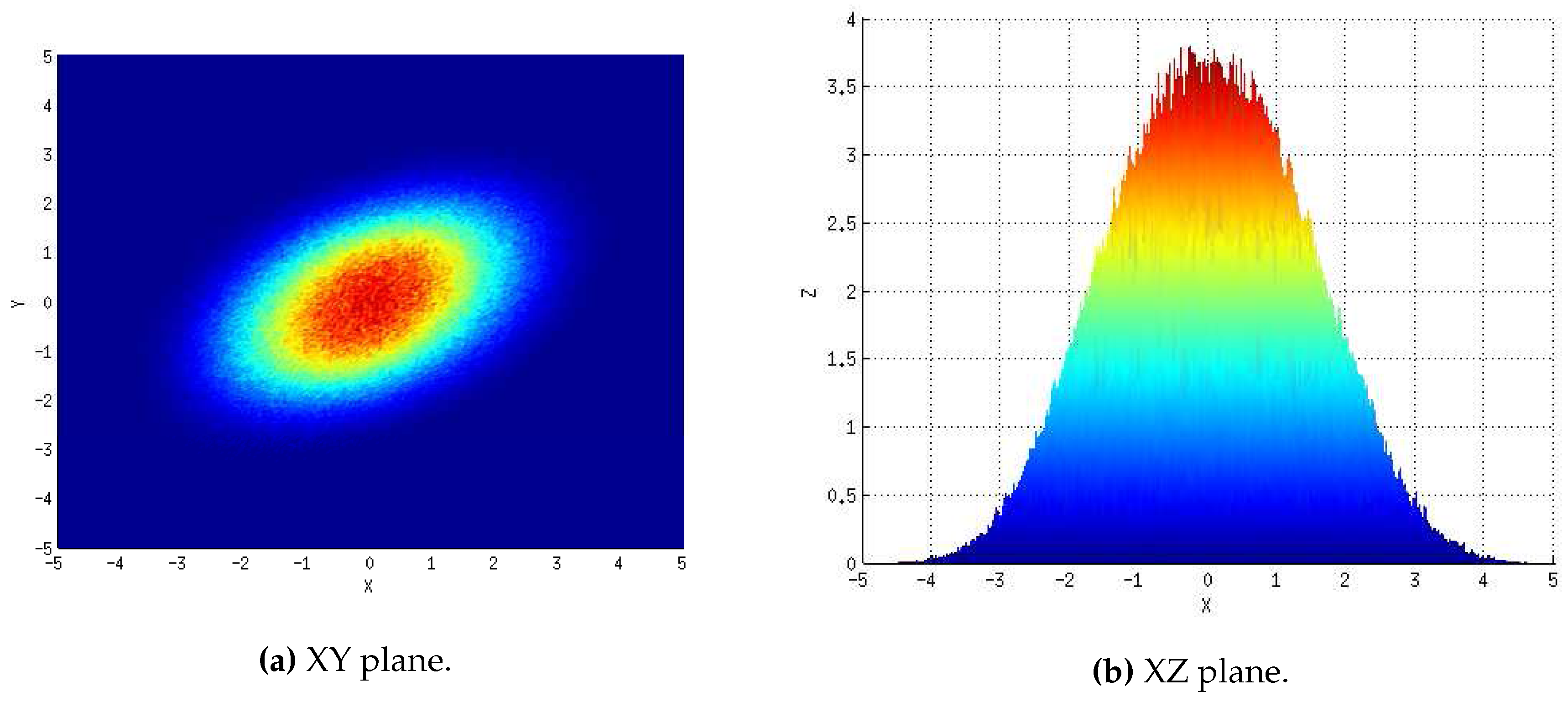
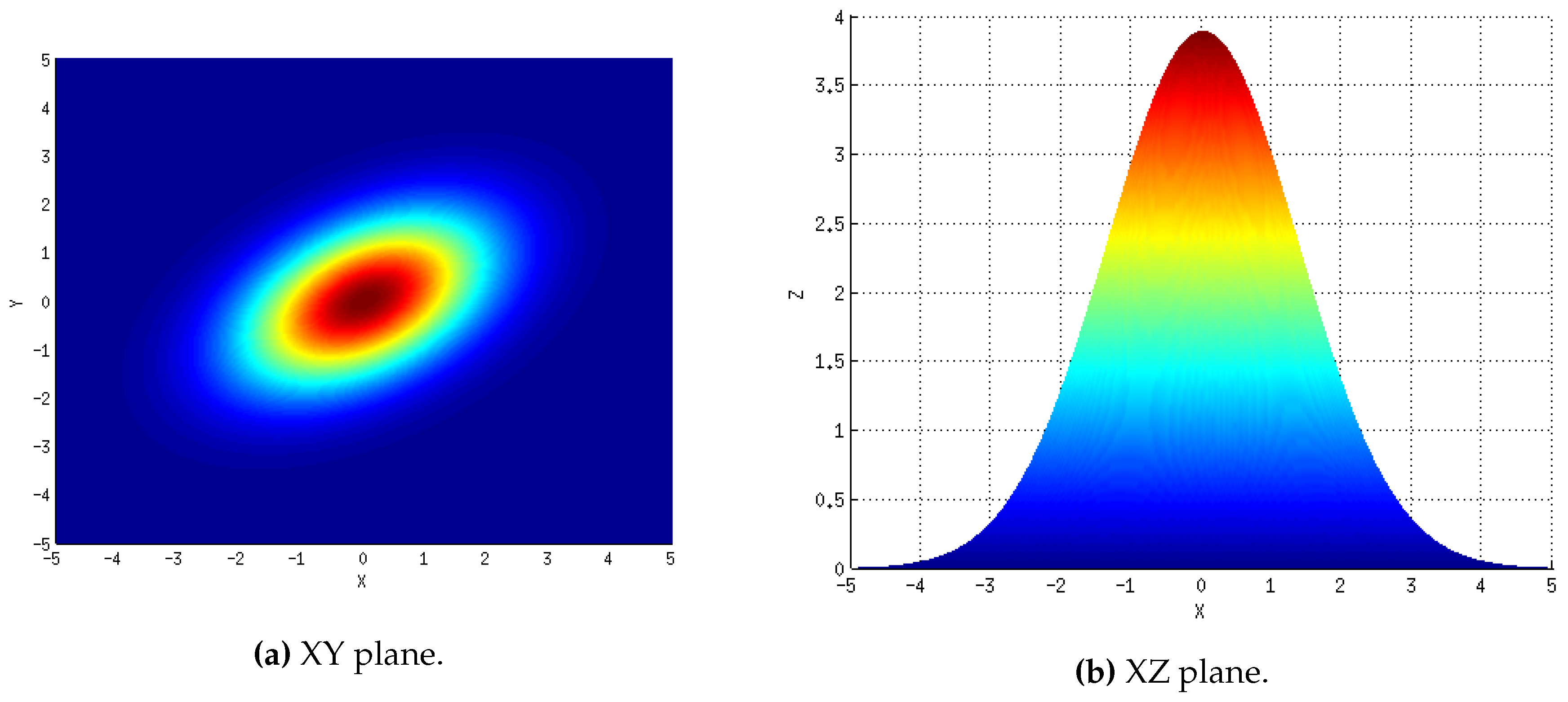
Additionally, to complement the validation information, the flux map of heliostat 290 gathered at ”DA” is shown in Figure 7. The XY and XZ planes are included, in kW/m², in Figure 7a,b, respectively. The equivalent information synthetically generated with M and $F^{*}$ is included in Figure 8 for comparison. Specifically, Figure 8a,b correspond to the XY and XZ planes, respectively. According to the XY plane, the overall shape generated over the receiver has successfully been replicated. However, as expected, the synthetic map is not a perfect replica: it is slightly thinner and features a higher peak as can be appreciated by comparing their XZ plane. Nevertheless, M has been able to estimate its overall distribution as indicated by the impressive similarity of the XY planes. Hence, the obtained results should be considered, at least, acceptable.

3.6. Model Deployment (MD)

At this point, the proposed methodology has successfully been executed and a compact representation of the considered field has been built. By studying only 30 heliostats in-depth, i.e., approximately $5.5\%$ of the field, it has been characterized for the target instant. Hence, by using M, a table with the parameters that describe the instantaneous flux maps of every heliostat, in terms of Equation (1), can be obtained. It is no longer necessary to store and/or access the ”real” data and the meta-model can be used, i.e., deployed, where required. For instance, this approach has successfully been used to test automatic heliostat aiming strategies in [34].

4. Conclusions

In this work, a new methodology for extensive heliostat field characterization has been proposed and described. It aims to facilitate the possibility of modeling a whole heliostat field, at a certain instant, by a reduced set of analytical expressions. They, which form what has been called as a ”meta-model”, are expected to estimate the parameters that define the overall shape of the flux map of every heliostat, according to a selected theoretical flux distribution. In simpler words, the methods describe how to take a consistent ”snapshot” of a heliostat field. Therefore, when successfully applied, an approximate and portable representation of the field can be obtained with a relatively reduced effort. This aspect also enhances the autonomy of researchers to build and share their own consistent synthetic datasets.

The proposed methodology, as defined in abstract terms, can be applied to either real or virtual fields without explicit requirements. However, aspects such as symmetry can significantly increase the possibility of success. A complete application example over a virtual field has also been included to complement the theoretical description. By studying only a subset of 30 heliostats out of 541, an instantaneous meta-model of the field has been built. An analytical and portable description of the field based on the meta-model has successfully been obtained and validated, which confirms its applicability. The only limits are what can precisely be modeled and what cannot, especially depending on acquisition conditions at ”DA”.

Finally, regarding potential future work, the proposed methodology will be used to characterize a real field in order to test new automatic aiming strategies. In addition, the formal generalization and application of the procedure to encompass a substantial set of instants, i.e., solar positions, will be considered. Upon success, its direct applicability to on-line automatic control would be of major interest.