1. Introduction
Gas turbine engines, which are among the most sophisticated devices, perform an essential role in industry. Detecting anomalies and eliminating faults during gas turbine maintenance is a great challenge since the devices always run under variable operating conditions that can make anomalies seem like normal. As a consequence, Engine Health Management (EHM) policies are implemented to help gas turbines run in reliable, safe and efficient state facilitating operating economy benefits and security levels [
1,
2]. In the EHM framework, many works have been devoted into anomaly detection and fault diagnosis in gas turbine engines. Since Urban [
3] first got involved in EHM research, many techniques and methods have been subsequently proposed. Previous anomaly detection works mainly involve two categories: model-based methods and data driven-based methods. Model-based methods typically includes linear gas path analysis [
4,
5,
6], nonlinear gas path analysis [
7,
8], Kalman filters [
9,
10] and expert systems [
11]. Data driven-based methods typically include artificial neural networks [
12,
13], support vector machine [
14,
15], Bayesian approaches [
16,
17], genetic algorithms [
18] and fuzzy reasoning [
19,
20,
21].
Previous studies are mainly based on simulation data or continuous observation data. Simulation data are sometimes too simple to reflect actual operating conditions as real data usually contains many interferences that make anomalous observations appear normal. This is particularly challenging for anomaly detection in gas turbines that operate under sophisticated and severe conditions. There are two possible routes for improving anomaly detection performance for gas turbines, the first one is from the perspective of anomalous data and the second one is from the perspective of a detection model.
On the one hand, anomalies occurring during gas turbine operation usually involve collective anomalies. A collective anomaly is defined as a collection of related data instances that is anomalous with respect to the entire data set [
22]. Each single datapoint doesn’t seem like anomaly, but their occurrence together may be considered as an anomaly. For example, when a combustion nozzle is damaged, one of the exhaust temperature sensors may record a consistently lower temperature than other sensors. Collective anomalies have been explored for sequential data [
23,
24]. Collective anomaly detection has been widely applied in domains other than gas turbines, such as intrusion detection, commercial fraud detection, medical and health detection, etc. [
22] In industrial anomaly detection, some structural damage detection methods are applied by using statistical [
25], parametric statistical modeling [
26], mixture of models [
27], rule-based models [
28] and neural-based models [
29], which can sensitively detect highly complicated anomalies. However, in gas turbine anomaly detection, these methods have some common shortcomings. For example, data preprocessing methods such as feature selection and dimension reduction are highly complicated when confronting gas turbine observation data, which greatly undermines the operating performance. Furthermore, many interferences included in the data such as ambient conditions, normal patterns changes, even sensor observation deviations produce extraneous information for detecting anomalies, usually concealing essential factors that may be critically helpful for detection. For instance, a small degeneration in a gas turbine fuel system may be masked by normal flow changes, thus hindering anomaly detection of a device’s early faults. Thus, some studies have focused on fuel system degeneration estimation by using multi-objective optimization approaches [
30,
31], which are helpful for precise anomaly detection in fuel systems.
On the other hand, detection models for gas turbines require both sensitivity and robustness capabilities. The sensitivity ensures a higher detection rate and the robustness ensures fewer misjudgements. The symbolic dynamic filtering (SDF) [
32] method was proposed and yielded good robustness performance in anomaly detection in comparison to other methods such as principal component analysis (PCA), ANN and the Bayesian approach [
33], as well as suitable accuracies. Gupta et al. [
34] and Sarkar et al. [
35] presented SDF-based models for detecting faults of gas turbine subsystems and used them to estimate multiple component faults. Sarkar et al. [
36] proposed an optimized feature extraction method under the SDF framework [
37]. Then they applied a symbolic dynamic analysis (SDA)-based method in fault detection in gas turbines. Next they proposed Markov- based analysis in transient data during takeoff other than quasi-stationary steady-states data and validated the method by simulation on the NASA Commercial Modular Aero Propulsion System Simulation (C-MAPSS) transient test-case generator. However, current SDF-based models usually adopt simulated data or data generated in laboratories, especially in the gas turbine domain. The performance of these methods remains unconfirmed with real data, for instance, from long-operating gas turbine devices that contains many flaws and defects, for which sensors may not always be available for data acquisition.
Considering that both solutions for improving the performance of gas turbine anomaly detection have their disadvantages, in this paper, we combine the two strategies by building a SDA-based anomaly detection model and processing collective anomalous sequential data in order to establish more sensitive and robust models and eliminate their intrinsic demerits. We then apply this method in anomaly detection for gas turbine fuel systems.
In this paper, the observation data from an offshore platform gas turbine engine are first partitioned into symbolic sequential data to construct a SDA-based model, finite state machine, which reflects the texture of the system’s operating tendency. Then two methods, an estimation-based model and a detection-based model, are proposed on basis of the sequential symbolic reasoning model. One method is more robust and the other is more sensitive. The two methods can be well integrated in different practical scenarios to eliminate irrelevant interferences for detecting anomalies. A comparison between collective anomaly detection, symbolic anomaly detection and our method is presented in
Table 1.
This paper is organized in six sections. In
Section 2, preliminary mathematical theories on symbolic dynamic analysis are presented. Then, in
Section 3 the data used in this study and symbol partition are introduced. The finite state machine training and the two anomaly detection models are proposed in
Section 4. Experimental results and a comparison between the two models from several perspectives are given in
Section 5 and a discussion and conclusions are briefly presented in
Section 6.
3. Data and Symbolization
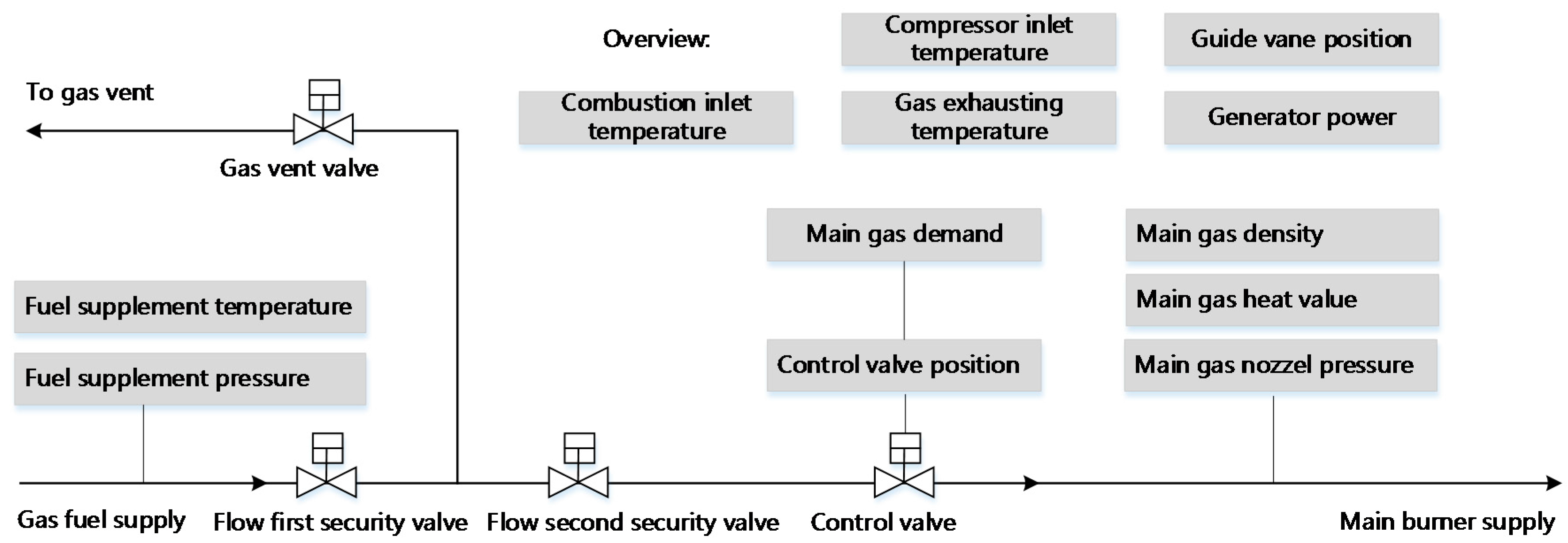
In gas turbine monitoring, all operation data observed by sensors are continuous. There is no observation that can acquire several discrete operating conditions automatically. Thus, in this section we focus on a symbol extraction method that can discretely represent different load condition patterns. After symbolization, many irrelevant interferences are dismissed. In this paper, the data resource is from a SOLAR, Titan 130 Gas Turbine. The parameters used are listed in
Table 2 below and an overview of the structure of the turbine fuel system is shown in
Figure 3.
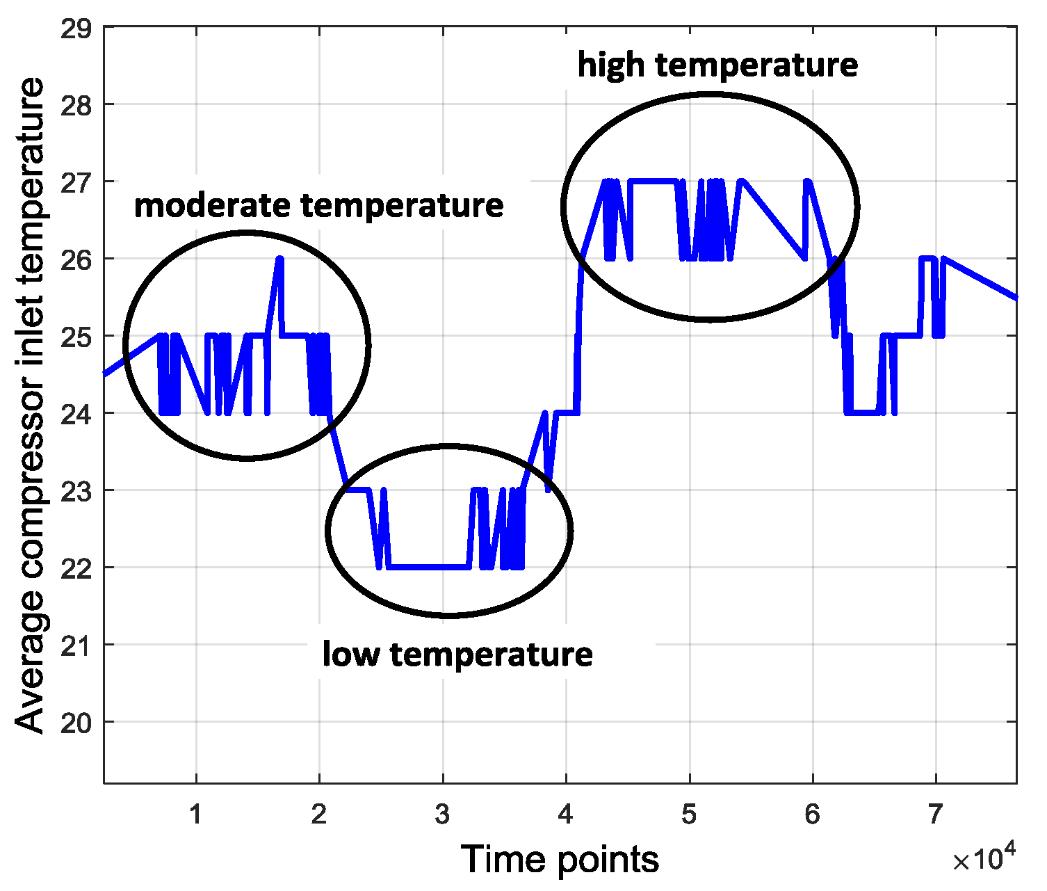
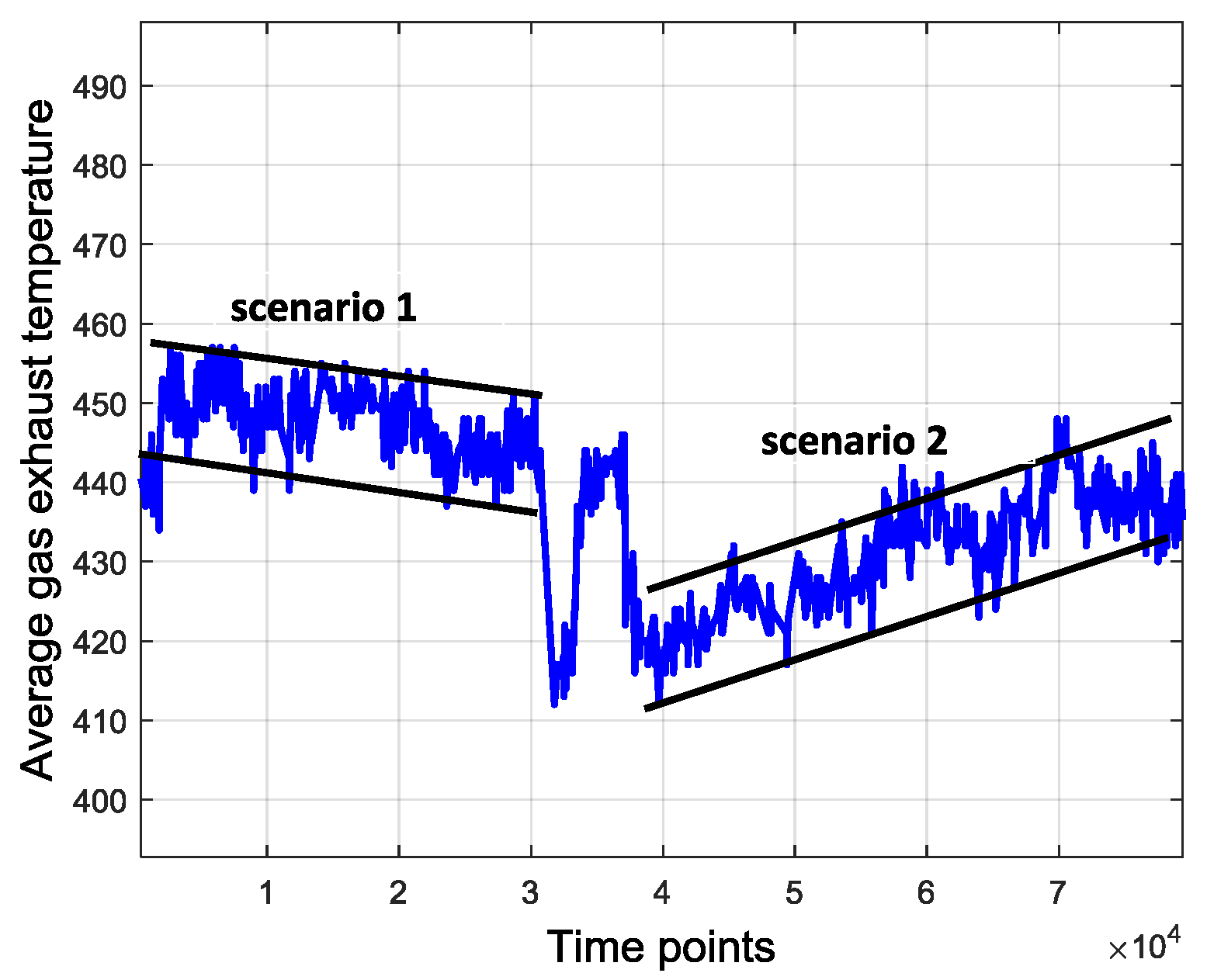
Original data contain many uncertainties and ambient disturbances. For example, the average combustion inlet temperature varies during daytime and at night, influenced by the atmospheric temperature that fluctuates over several days. This tendency is shown in
Figure 4. Besides, the operating parameters of the gas turbine also have uncertainty, even under the same operating pattern.
Figure 5 shows the uncertainty of the average gas exhaust temperature. It suggests that both in scenarios 1 and 2, the average gas exhaust temperature has an uncertainty boundary around the center line. All these factors may influence the device operation and data processing. The disturbances and uncertainties are usually extraneous and redundant, which interferes with the anomaly detection. Therefore, one way to eliminate such interferences is data symbolization.
Many strategies for data symbolization or discretization have been proposed and were well discussed in previous papers [
39,
40,
41]. In summary, two kinds of approaches—splitting and merging—can be used in data symbolization. A feature can be discretized by either splitting the interval of continuous values or by merging the adjacent intervals [
36]. It is very difficult to apply the splitting method in our study since we cannot properly preset the intervals. Therefore, a simple merging-based strategy is adopted for data symbolization. We apply a cluster method to symbol extractions—K means (KM) cluster method. The main reason is that in a FSM, the number of hidden states and visible symbols are both finite and KM initially has a specific cluster boundary and expected cluster numbers. Samples in a cluster are regarded as the same symbol. There are seven clusters that correspond to seven different load conditions as shown in
Table 3, so K is equal to 7 for the KM model.
The purpose of the KM method is to divide original samples into k clusters, which ensures the high similarity of the samples in each cluster and low similarity among different clusters. The main procedures of this method are as follows:
- (1)
Choose k samples in the dataset as the initial center for each cluster, and then evaluate distances between the rest of the samples and every cluster centers. Each sample will be assigned to a cluster to which the sample is the closest.
- (2)
Renew the cluster center through the nearby samples and reevaluate the distance. Repeat this process until the cluster centers converge. Generally, distance evaluation uses the Euclidean distance and the convergence judgement is the square error criterion, as shown in Equation (7):
where
E is sum error of total samples,
P is the position of the samples and
is the center of cluster
. Iteration terminates when E becomes stable, which is less than 1 × 10
−6.
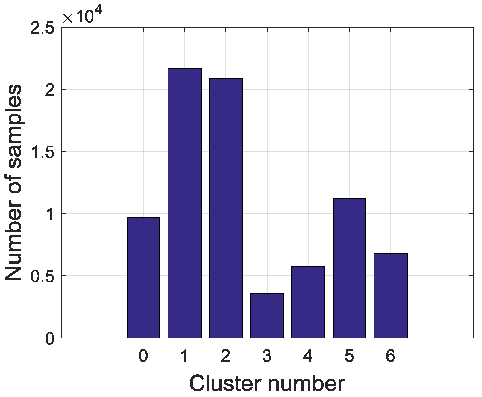
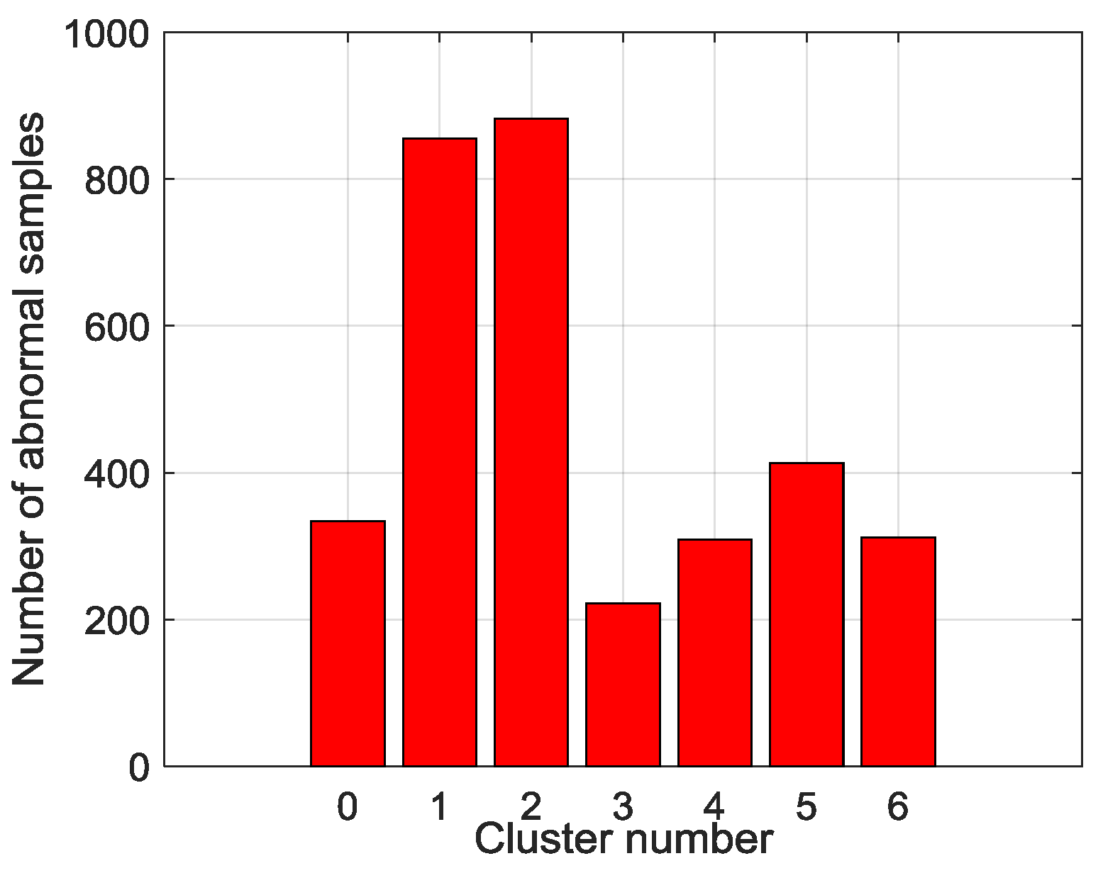
Therefore, the final clusters and samples are converted from continuous variables into discrete visible symbols. In this study, altogether 79,580 samples that are divided into seven symbols. The sampling interval is 10 min and symbol extraction results are shown in
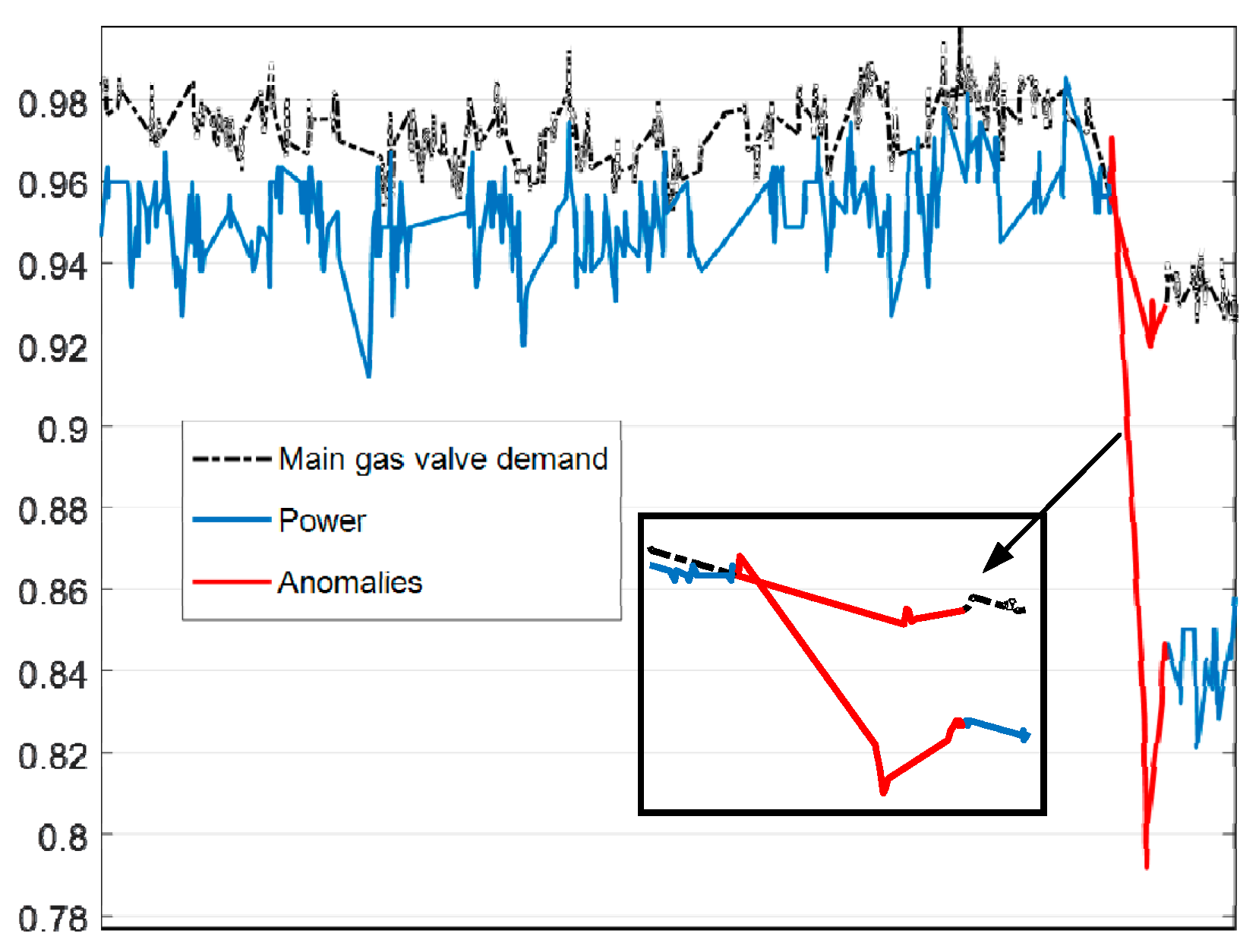
Figure 6. The most frequent symbols are Steady in high load (SHL) and Steady in low load (SLL). The intermediate ones are Flow rise in low load (FRLL), Flow rise in high load (FRHL), Flow drop in low load (FDLL) and Flow drop in high load (FDHL). The least frequent symbol is Fast changing condition (FCC). There are 3327 samples labeled as anomalies and the distribution of the abnormal samples is shown in
Figure 7. All of the abnormal labels are derived manually from the device operation logs and maintenance records. To simplify our modeling, we classify all kinds of anomalies or defects in records into one class—anomaly. After symbolization, we use these symbols generated by KM cluster method to construct a FSM to measure whether a series of symbols are on normal conditions or on an abnormal one.
4. FSM Modeling and Anomaly Detection Methods
The finite state machine, widely applied in symbolic dynamic analysis, has shown great superiority in comparison to other techniques [
30,
31]. Therefore, the main tasks of establishing a sequential symbolic model in gas turbine fuel system anomaly detection are to build a FSM to estimate posterior probabilities of sequences and to build detection models to detect the abnormality of sequences. Before this, however, the discrete symbols extracted in
Section 3 need to be sequenced into series, time series segments, of length
T.
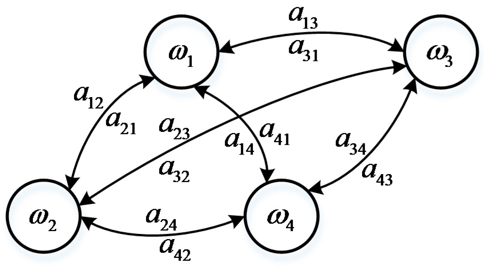
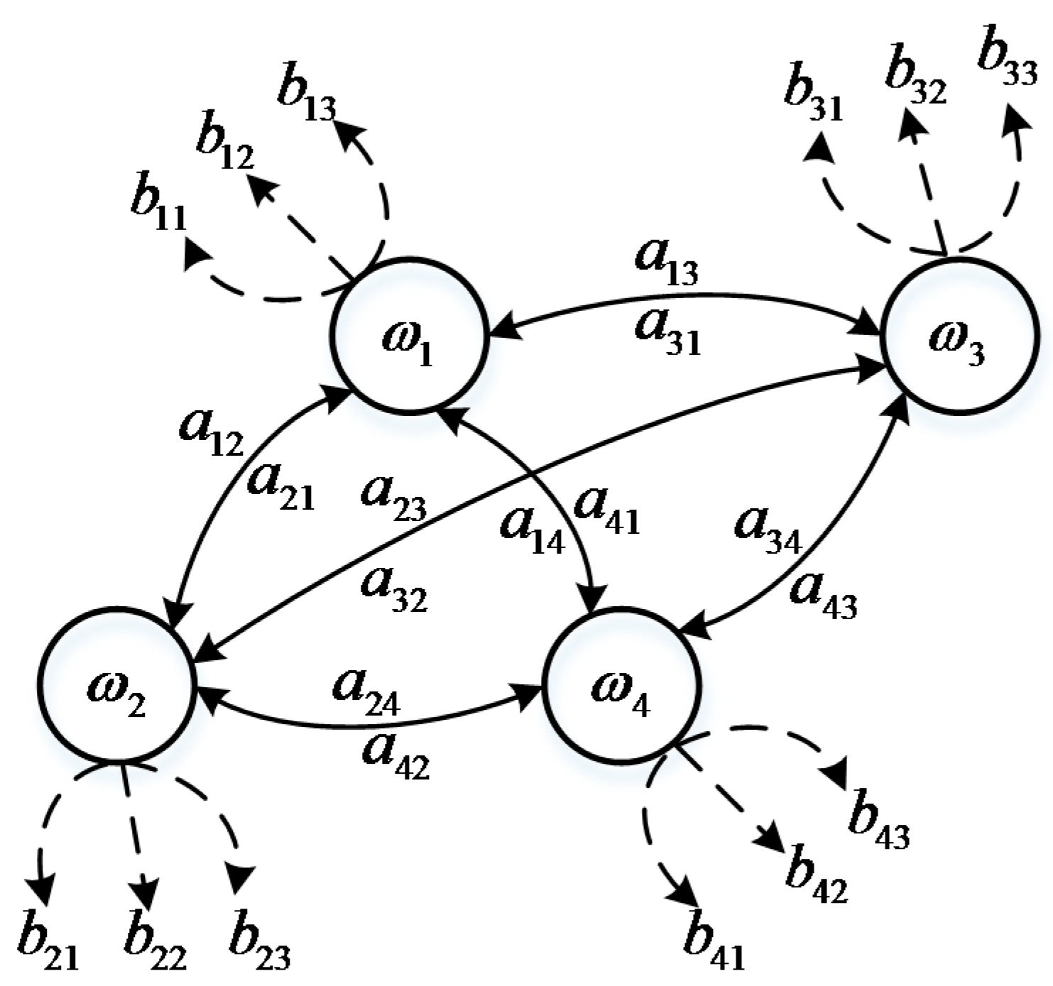
For FSM modeling, one aspect of this work is to determine several parameters. There are five states defined in this model: normal state (NS), anomaly state (AS), turbine startup (ST+), turbine shutdown (ST-) and halt state (HS). Actually, anomaly is a hidden state that is usually invisible during operation compared to the other four states. Till now, we have defined the model structure of the FSM which contains five states and seven visible symbols. For any moment, there are seven possible symbols in a state that could be observed with probability . is the probability that a state transfers from one to another. When the operating pattern changes reflected by symbols or hidden states at a structural level, the device might experience an anomaly that is easier to observe. This thus satisfies the basic idea of anomaly detection, finding patterns in data that do not conform to expected behavior.
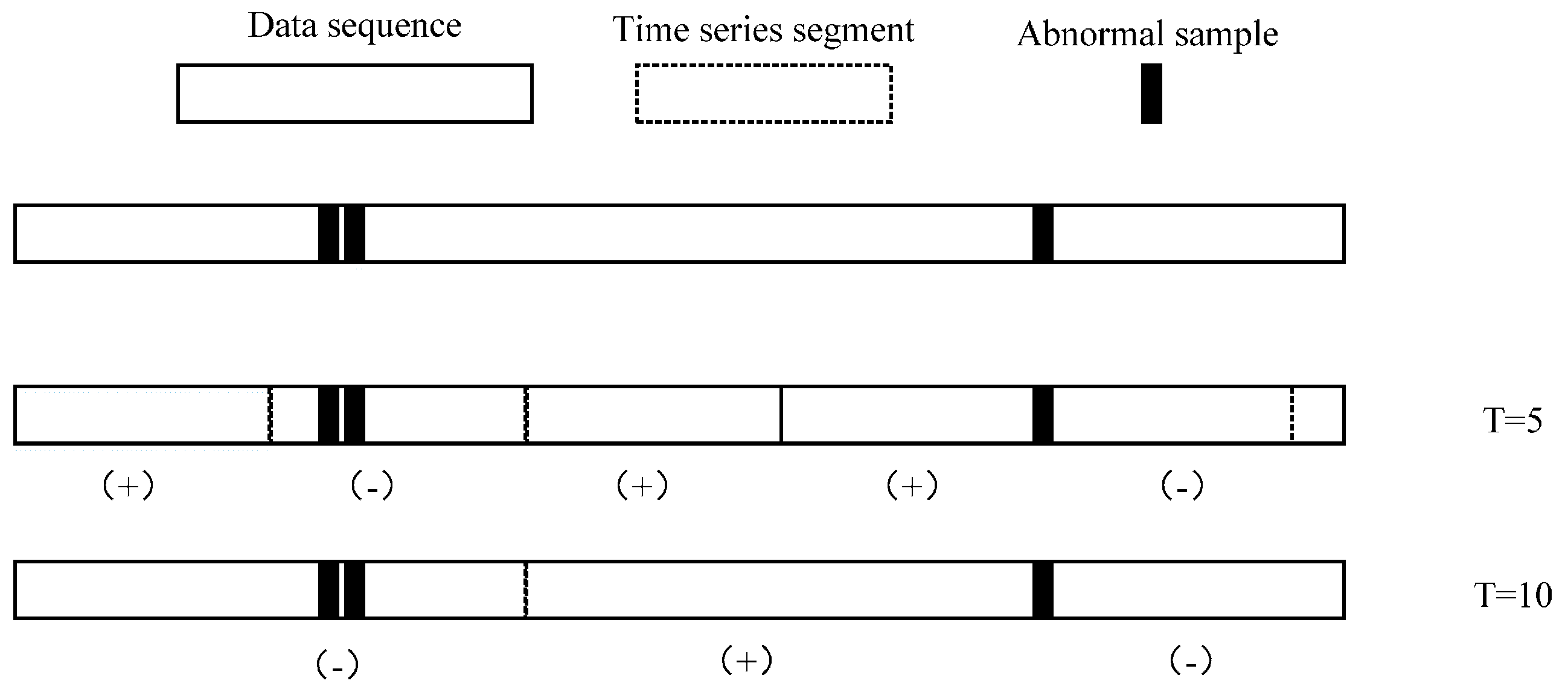
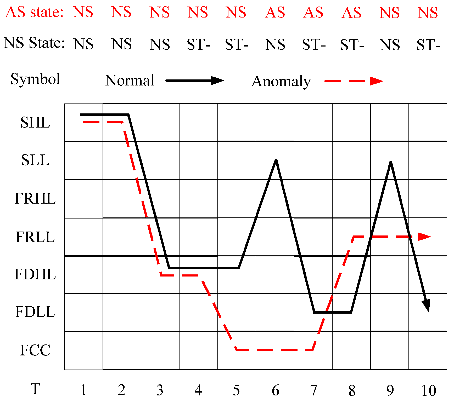
Another concern about FSM modeling is how long the time series are, which can be efficiently involved in the transfer and activation probability estimation.
Figure 8 shows that different lengths
T of segments may lead to different classification label results. A segment is defined as an anomaly only if it contains at least one abnormal sample. This classification suggests that the time series in
T = 5 and
T = 10 are significantly different.
It is difficult to primordially define a proper T that can be applied well in parameter estimation and anomaly detection, so another way we take is to optimize length T recursively until it has the best performance in the anomaly detection section. We declare that in actual data preprocessing, time series are generated by a sliding window with length T in order to ensure that the size of time series can match the original dataset, which means the total number of time series is 79581-T.
For anomaly detection, two strategies are used: an estimation-based model and a decoding-based model. The estimation-based model is that we use FSM to calculate the probability of a symbol sequence. In this case, FSM is built by the training data precluding abnormal samples, so the abnormal sequences contained in the testing data will have very low probabilities through calculation. The decoding-based model is that we use a FSM to decode a most probable state sequence which generates an observed symbol sequence. If the estimated state sequence contains anomaly states (AS), the symbol sequence is judged to be an anomaly.
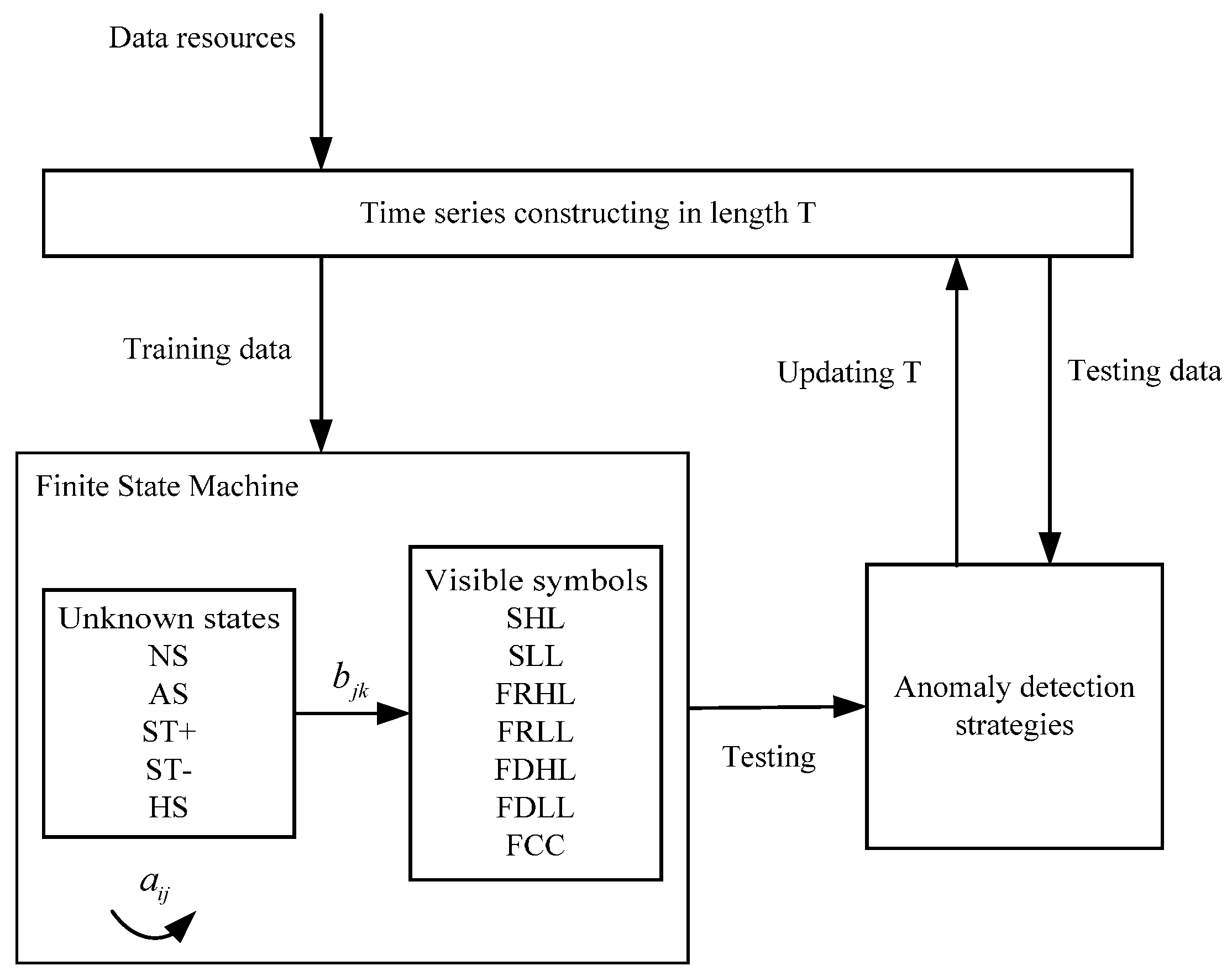
According to the aforementioned contents, the schematic of a FSM modeling is shown in
Figure 9, as illustrated below. First, data are sequenced into a pool of time series by an initial sliding window with length T. Then data are divided into two parts: training data and testing data. The training data are used to construct a FSM, to estimate transfer and activation probabilities of unknown states and visible symbols. The testing data are used to evaluate the FSM performance. After modeling the FSM, performance will be tested through two anomaly detection strategies—the decoding-based model and the estimation-based model. Length
T will be updated until the models and the FSM achieve the best performance.
4.1. Training a FSM
The main task of training a FSM is to estimate a group of transfer probabilities
and activation probabilities
from a pool of training samples. In this study, Baum-Welch algorithm [
41] is used in estimation. The probability
is deduced in Equation (6). Therefore, an estimated transfer probability
is described as:
Similarly, estimation of activation probability
is described as:
where expectation activation probability of
on state
is
and the total expectation activation probability on state
is
, l is number of symbols.
According to the analysis above
can be gradually approximated by
through Equations (8) and (9) until convergence. The pseudocode of the estimation algorithm is shown in Algorithm 1 below. The first
are generated randomly at the beginning. Hence we can evaluate
using
estimated in the former generation. We repeat this process until the residual between
and
is less than a threshold
and then the optimized
are used in the FSM.
| Algorithm 1. Procedures of estimation. |
| | Input: |
| | Initial parameters , Training set , convergence threshold , |
| | Output: |
| | Finial estimated FSM parameters |
| 1 | Loop |
| 2 | Estimating by in Equation (8) |
| 3 | Estimating by in Equation (9) |
| 4 | |
| 5 | |
| 6 | Until |
| 7 | Return , |
4.2. Anomaly Detection Based on the Estimation Strategy
An estimation strategy is used in anomaly detection of FSM in this part, which is inspired by anomaly detection approaches. Anomaly detection is defined as finding anomalous patterns in which data do not relatively satisfy expected behavior [
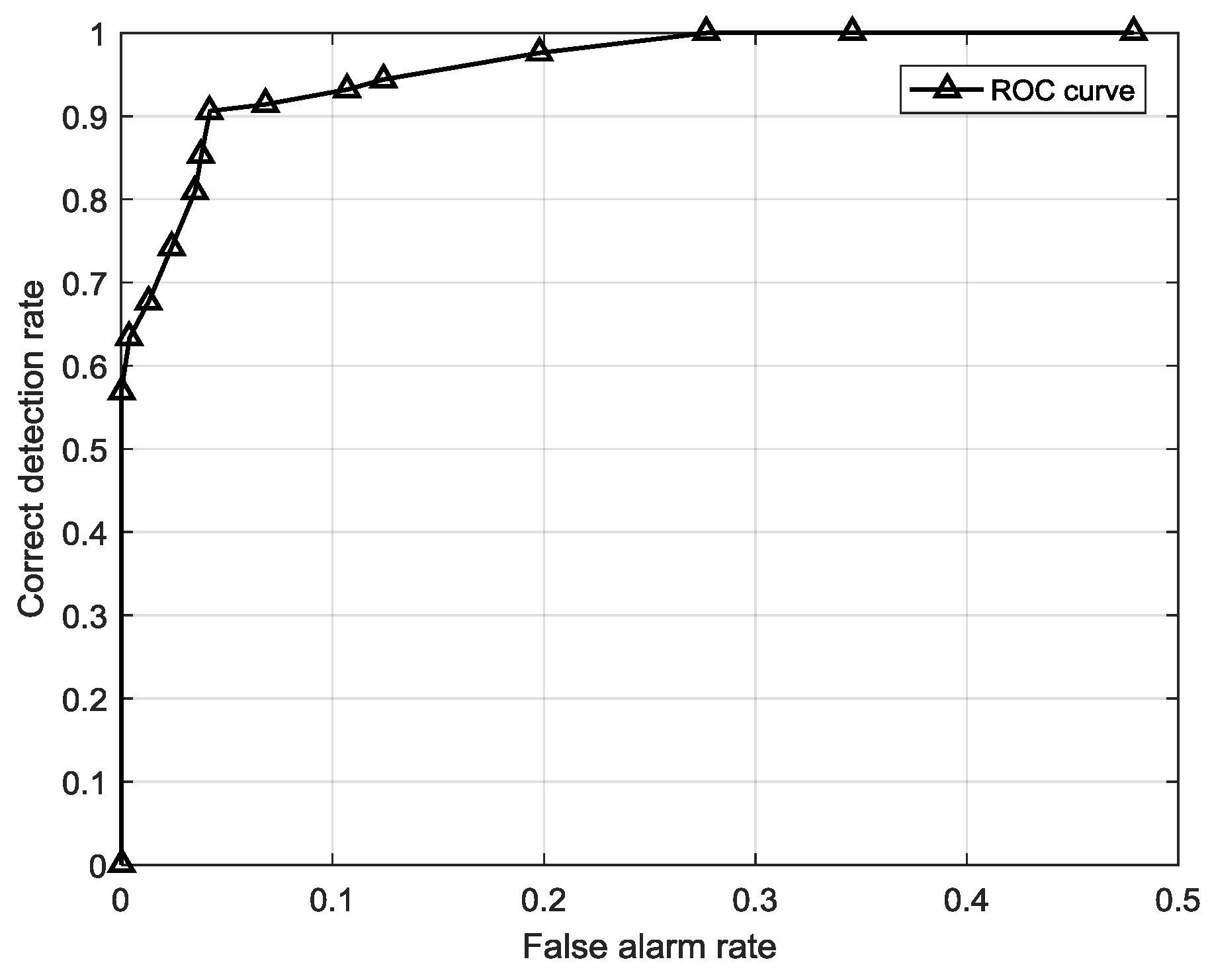
22]. The FSM estimation strategy calculates the posterior probabilities of the symbol sequences generated by FSM. It can detect anomalies efficiently if it has been built from normal data. Therefore, this strategy conforms to the basic idea of what anomaly detection does. In this strategy, FSM is utilized to establish an expected pattern and the estimation process involves finding the nonconforming sequences, in other words, the anomalies.
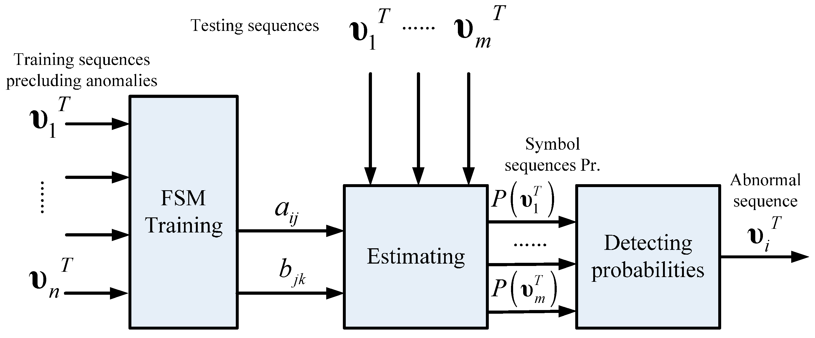
Figure 10 illustrates the schematic of anomaly detection using the estimation strategy. In order to establish an expected normal pattern, the training data used in FSM modeling are utterly normal sequences. Parameters
are estimated by FSM training, which indicates the intrinsic normal pattern recognition capability contained in these parameters, hence, the model estimation probabilities of testing symbol sequences in which abnormal sequences are included. Probabilities in normal sequences will be much higher than that in abnormal ones, so the detection indicator is actually a preset threshold that judges the patterns of test sequences.
The probability of a symbol sequence generated by a FSM can be described as:
where
r is the index of state sequence of length
T,
. If there are, for instance, c different states in this model, the total number of possible state sequences is
. An enormous amount of possible state sequences need to be considered to calculate the probability of a generated symbol sequence
, as shown in Equation (10). The second part of the equation can be descried as:
The probability
is continuous and chronological multiplication. Assume that activation probability of a symbol critically depends on the current state, so the probability
can be described in Equation (12) and then Equation (13) is the other description of Equation (10):
However, the computing cost of the above equation is
which is too high to finish this process. There are two alternative methods that can dramatically simplify the computing process, a forward algorithm and a backward algorithm, which are depicted by Equations (5) and (6), respectively. The computing cost of these algorithms are both
, that is
times faster than the original strategy. Algorithm 2 shows the detection indicator based on the forward algorithm. Initialize
, training sequences
precluding anomalies,
,
t = 0., then update
until
t =
T and the probability of
is
. If the probability is higher than the preset threshold, then the symbol sequence is classified in the positive, normal class. Otherwise the symbol sequence is classified in the negative, anomalous class.
| Algorithm 2. Anomaly detection based on the estimation strategy. |
| | Input: |
| | , , sequence , , threshold |
| | Output: |
| | Classification result |
| 1 | For |
| 2 | |
| 3 | Until |
| 4 | Return |
| 5 | If |
| 6 | |
| 7 | Else |
| 8 | Return |
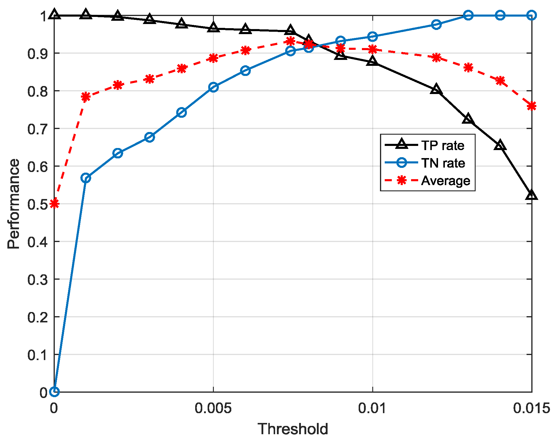
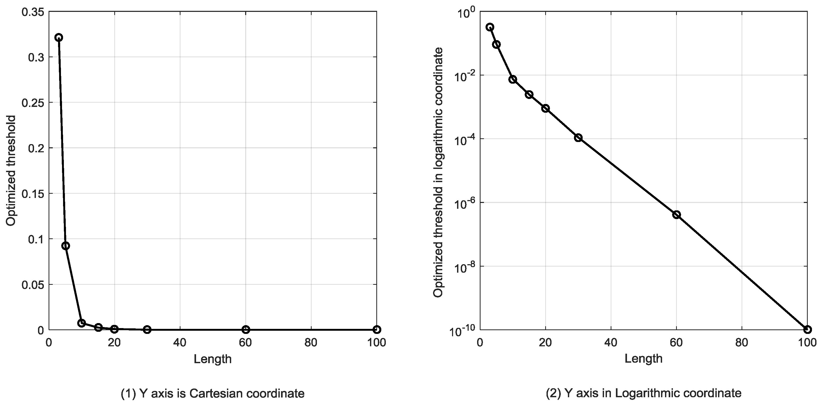
There are two points to be mentioned. In the first place, the decision judgement is very simple for use of anomaly detection by threshold . This convenience is ascribed to the normal pattern constructed by FSM. The probabilities estimated from FSM intuitively simulate the possibilities of the symbol sequences emerging in a real system. Furthermore, the performance of this strategy is not only dependent on the efficiency of the trained FSM, but also on the proper threshold. Therefore, in the modeling process, we optimize the threshold by traversing different values in order to get the highest overall accuracy of normal and abnormal sequences.
4.3. Anomaly Detection Based on the Decoding Strategy
Compared to the estimation strategy, a FSM can detect anomalies too if it can recognize whether there are hidden anomalous states in sequences. Fortunately decoding a state sequence is available in FSM so another way to detect anomalies is to decode a symbol sequence to state sequence and then find whether the state sequence contains abnormal states. Unlike the previous estimation strategy, the decoding strategy is a sort of, somehow, optimization algorithm in which a searching function is used.
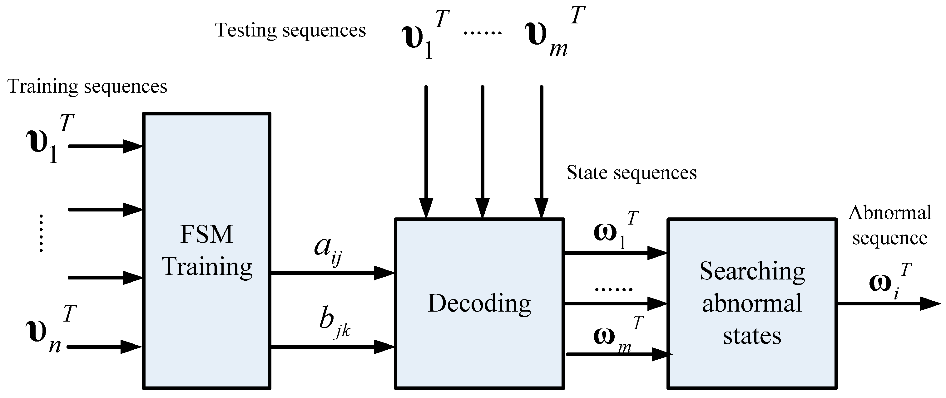
Figure 11 illustrates the schematic of anomaly detection using the decoding strategy. In this strategy, FSM is trained by all sequences that contain both normal and abnormal sequences so the FSM reflects the system that may run on normal or abnormal patterns. After that, the decoding process involves searching for the most probable state sequence that the symbol sequence corresponds to. A greedy-based method is applied in searching in each step so the most possible state is chosen and is added to the path. The final path is the decoded state sequence. Finally, the model judges a symbol sequence by its state sequence on whether it contains anomaly states.
Algorithm 3 shows the procedures of the decoding-based anomaly detection strategy. Initialize parameters
, testing sequence
,
, and path. Then, update
and in each moment
t, traverse all state candidates and the most possible state in this moment is the one who makes
biggest and then add the state into the path until the end of the sequence. After that, scan the decoded state sequence if there is at least one anomaly state (AS), then the observed sequence is classified in the negative, anomalous class, otherwise classified in the positive, normal class.
| Algorithm 3. Anomaly detection based on the decoding strategy. |
| | Input: |
| | , , , , |
| | Output: |
| | Classification result |
| 1 | For |
| 2 | |
| 3 | For |
| 4 | |
| 5 | Until |
| 6 | |
| 7 | Add to |
| 8 | Until |
| 9 | If contains state (AS) |
| 10 | |
| 11 | Else |
| 12 | Return |
Compared to the estimation strategy, the decoding strategy has some advantages and disadvantages. First of all, the detection indicator based on the decoding strategy may help the anomaly detection system sensitivity improve, meaning that it can precisely warn of an anomaly once it occurs. Besides, it helps system locate anomaly emerging time in high resolution. For example, a sequence contains 10 samples and the sample interval is 10 min so the length of the sequence is 100 min. If the sequence is abnormal and the two system, estimation-based model and decoding-based model, both alert, the latter can provide a more precise anomaly occurrence time, for instance, in 20 min and 60 min possibly but the former can only provide a probability that an anomaly may have occurred. However, this point may also be a disadvantage of the decoding strategy due to the lack of robustness. This detection strategy is a local optimization algorithm that may reach a local minimum point that is actually not the global optimized solution. It may have searched an utterly different state sequence than the real one. Furthermore, error rate accumulates with the growth of the searching path, particularly for a longer length T, and the false positive rate may be very high, meaning that many normal sequences are classified as anomalies, so the length of the sequence is a critical factor for detection performance. It indicates the robustness performance of the models. This issue will be analyzed in the next section.
6. Conclusions
The essential issue of anomaly detection is how to detect sensitively and effectively when and how an anomaly would happen. Conventional anomaly detection methods for points or collective anomalies are mostly established based on continuous real-time sensor observations. Noise, operating fluctuation or ambient conditions may be all contained in raw data, which make anomalous observations appear normal. The anomalous features often hide in the structural data which reflects various patterns of the device operating. Thus, we first partitioned the original data into classes by using K-means clustering and symbolized each class to construct a sequence-based feature-structure which intrinsically represents the operating patterns of a device. Second, we built the core computing unit for anomaly detection, finite state machine, on a large quantity of training sequential data to estimate posterior probabilities or find most probable states. Two detection models were generated, an estimation-based model and decoding-based model. The two models on anomaly detection for gas turbine fuel system have their own advantages and weakness, concretely concluded as follows:
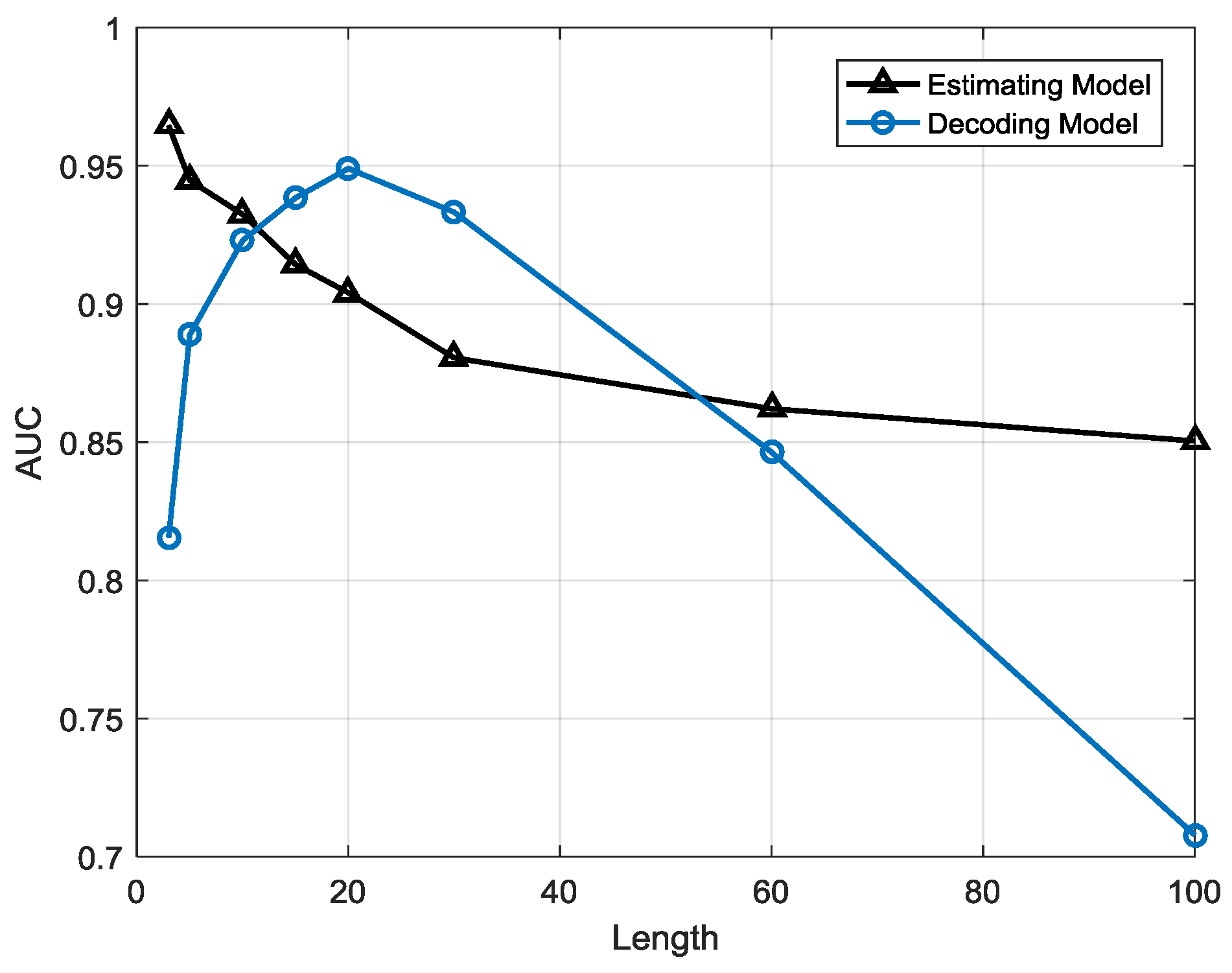
- (1)
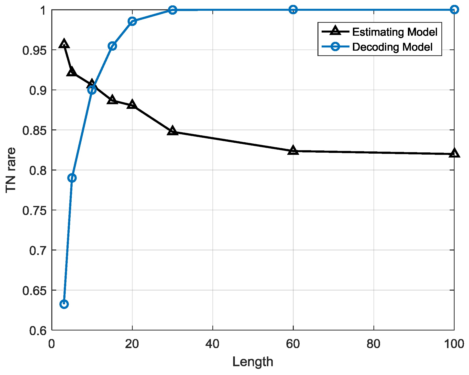
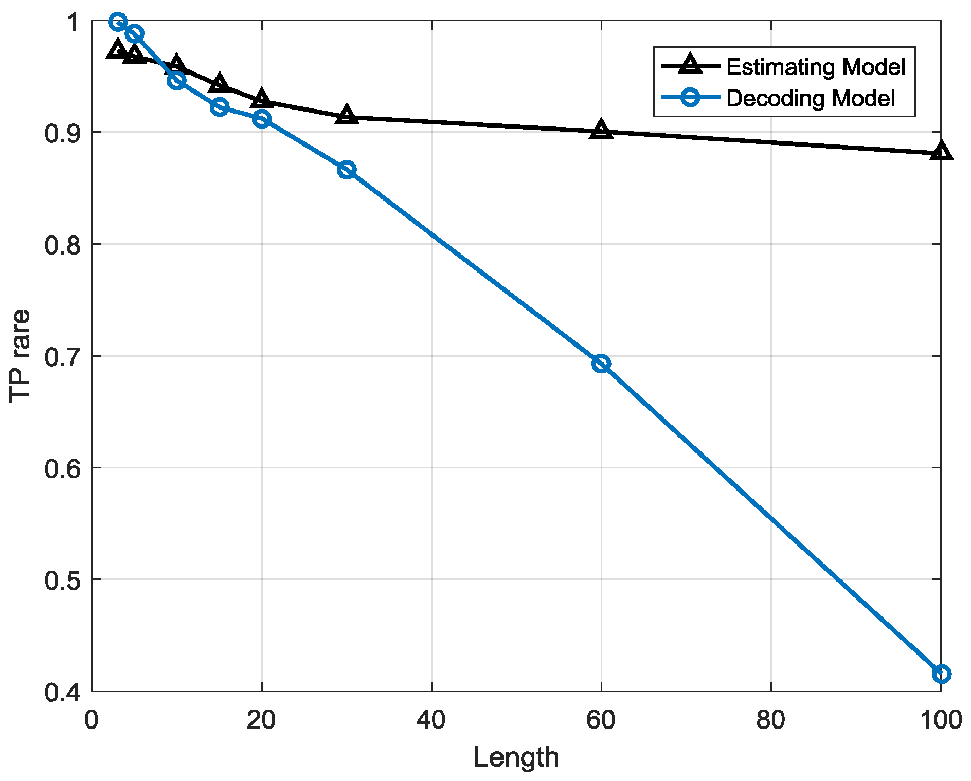
The estimation-based model has strong robustness since the performance is highly stable when the sequence length is growing. However, in the decoding-based model, the performance varies with different sequence lengths. The anomalous sequences are easier to detect in longer lengths than in shorter one, but there will be a higher false alarm rate at longer lengths, which means many normal sequences are misclassified as anomalies.
- (2)
The decoding-based model can help us to locate anomalies occurring point with a high time resolution, which means it can tell us precisely what symbol points are in an anomalous state rather than only probabilities of sequences made by the estimation-based model.
The estimation-based model is more suitable for anomaly detection in gas turbine fuel systems when the observation window is less than 1 h or over 8 h, whereas the decoding-based model is more suitable when the observation window is between 1 and 8 h, so it may help people choose the most efficient detection model for different demands.
Further work may be concentrated on algorithm optimization and application extension. As is described above, the decoding-based model uses a local searching algorithm which may cause high deviation in some circumstances, though it could be operated at a high computing speed, so the algorithms need to be optimized. We also need to apply this method to other domains of gas turbine anomaly detection, such as gas path, combustion components, etc. All of these need further attention.


