Measurement of Line-to-Ground Capacitance in Distribution Network Considering Magnetizing Impedance’s Frequency Characteristic

State Key Laboratory of Power Transmission Equipment & System Security and New Technology, Chongqing University, Chongqing 400044, China
*
Author to whom correspondence should be addressed.
Energies 2017, 10(4), 477; https://doi.org/10.3390/en10040477
Submission received: 1 February 2017
/
Revised: 21 March 2017
/
Accepted: 27 March 2017
/
Published: 3 April 2017
(This article belongs to the Special Issue Electric Power Systems Research 2017)
Abstract
:Signal injection method (SIM) is widely applied to the insulation parameters’ measurement in distribution network for its convenience and safety. It can be divided into two kinds of patterns: injecting a specific frequency signal or several frequencies’ groups, and scanning frequency in a scheduled frequency scope. In order to avoid the disadvantages in related researches, improved signal injection method (ISIM), in which the frequency characteristic of the transformer magnetizing impedance is taken into consideration, is proposed. In addition, optimization for signal injection position has been accomplished, and the corresponding three calculation methods of line-to-ground capacitance has been derived. Calculations are carried out through the vector information (vector calculation method), the amplitude information (amplitude calculation method), the phase information (phase calculation method) of voltage and current in signal injecting port, respectively. The line-to-ground capacitance is represented by lumped parameter capacitances in high-voltage simulation test. Eight different sinusoidal signals are injected into zero-sequence circuit, and then line-to-ground capacitance is calculated with the above-mentioned vector calculation method based on the voltage and the current data of the injecting port. The results obtained by the vector calculation method show that ISIM has a wider application frequency range compared with signal injection method with rated parameters (RSIM) and SIM. The RSIM is calculated with the rated transformer parameters of magnetizing impedance, and the SIM based on the ideal transformer model, and the relative errors of calculation results of ISIM are smaller than that for other methods in general. The six groups of two-frequency set are chosen in a specific scope which is recommended by vector calculation results. Based on ISIM, the line-to-ground capacitance calculations through the amplitude calculation method and phase calculation method are compared, and then its application frequency range, which can work as a guidance for line-to-ground capacitance measurement, is concluded.
1. Introduction
In distribution network, the number of grounding fault reaches 70% in all types of system faults, and over 70% of them are transient faults [1]. Self-healing plays an important role in distribution network [2,3,4,5,6,7,8]. The systems, which have been effectively grounding, protect themselves by switching breakers when grounding faults occur. However, resonant earthed system (namely ineffectively grounded system [9,10,11,12]) could compensate faulting current quickly by adjusting the resonance deviation υ of network through regulating the arc suppression coil. This would make an improvement of the withstanding ability of distribution network and guarantee a safe and reliable power system.
As the guidance of regulating arc suppression coil, the insulation parameters of distribution network mainly are [9,10,11,12,13,14,15,16,17,18,19,20,21,22]: line-to-ground stray capacitance and leakage resistance. Meanwhile, the line-to-ground stray capacitance is the key factor, which affects the compensation ability of the system and the performance of arc suppression coil dynamic regulation [9,10]. Besides, the capacitance can be utilized to improve the performance of fault detection in distribution networks [13,14,15] and the suppression of unbalanced voltage in neutral point [16]. In practice, the capacitive current of the system is often calculated by measuring line-to-ground capacitance. The common measurements are: artificial single-phase metal earth fault test [9,10], biased capacitance method [17], tuning through adjustable arc suppression coil [19,20,21,22,23,24,25,26,27], identification through recorded fault signal [28,29] and injecting signal into zero sequence of system (namely SIM) [9,10,11,21,22].
However, problems exist in both the artificial single-phase metal earth fault test and the biased capacitance method, such as earth fault and endangering the safety of operator. The tuning method gets line-to-ground capacitance via measuring neutral-to-ground voltage and then solving equations or just obtaining it from tuning curves, which will inevitably reach the resonance point of system in the tuning process. The insulation parameters extracted based on the recorded fault waveform of the transmission line can be classified as passive measurement [28,29], which could not be able to suppress earth fault automatically when earth fault occurs. The SIM is a widely used method for line-to-ground capacitance measurement. This method requires the amplitude and phase information of injecting current and returned voltage to calculate line-to-ground capacitance. And the method has no influence upon the safe operation of the system because its injection power is low. Besides, the SIM device is simple and could get a relatively accurate result of line-to-ground capacitance. The related researches mainly focus on the wave pattern of injecting current signal and the injection pattern of current signal. The wave patterns of injecting current signal are single frequency [9,10,11,22] and several frequencies [9,10]. The single-frequency injection which operates calculation through the information of a certain frequency, can be divided into constant frequency injection [10,11,22] and variable frequency injection (namely frequency scanning method) [9,10]. The injection pattern of current signal is: the open-delta secondary side of potential transformer (PT) in bus [10,21] and the secondary winding of arc suppression coil [9,22].
The researches described above have vastly enlarged the technology of line-to-ground capacitance measurement and provided a lot of practical methods. The SIM is a promising method for its convenience and accuracy upon measurement of line-to-ground capacitance. For the traditional measurement, the frequency characteristic of the injecting transformer magnetizing impedance (represented as Zm) is treated as an ideal model, because Zm is assumed as a massive value and could be treated as open-circuit. However, it is found that the injecting transformer is easy to be saturated at low frequency in practice, even if the injecting power is much lower than the rated capacity of injecting transformer. Besides, normally, the rated capacity of the injecting transformer is low, which is unable to avoid the saturation. Thus, if the saturation of the injecting transformer is not considered in the final calculation based on the test data, it is difficult to find the proper injection frequency range or frequency group during the measurement [9,10,11,21,22]. And the system error would also be increased. In addition, the frequency scanning method, applied widely in practice, needs long measuring times, and requires well output performance and high respond speed of injection signal source, which makes it hard to meet the requirement of real-time measurement. Moreover, several frequencies, injected at the same time, demand for the excellent injection signal source because the desired waveform is always non-standard. Thus, the constant frequency injection is applied in this paper for its convenience and suitable for realizing real-time measurement.
For the traditional injection patterns [9,10,21,22], the power is injected to the secondary side of the transformer such as PT or arc suppression coil with a high turn ratio. However, for the presented method as Figure 1, the power is injected to an injecting transformer with a 1:1 turn ratio. Thus, the current in the primary side of the transformer, induced by the current injected in the secondary side of the transformer for the traditional method, is lower than that for the presented method. Hence, the presented method could mitigate the influence of the noise upon the current signal and have a high signal-to-noise ratio. Besides, according to the investigation carried out by ourselves, it is found that most of the arc suppression coil in China is the multi-tap arc suppression coil. Only the inductance is presented for a certain resonance deviation of the system, which means the real turn ratio is difficult to identify. Therefore, the accuracy of the measured voltage in the secondary side of the injecting transformer may be influenced by the unidentified real turn ratio. When the current signal is injected through the open-delta of the 10 kV PT in bus, the measurement accuracy may be affected by the magnetizing impedance because the injecting transformer is normally small in size, and prone to be saturated. In addition, the injecting transformer is normally installed in the switchgear. The high injected power may cause the short-circuit fault of the 10 kV bus. Hence, injecting through the open-delta side of the voltage transformer is a potential threat to the safe operation of the entire switchgear.
Based on the analysis above, a new line-to-ground capacitance measurement method, namely ISIM, is presented in this paper, which is developed from SIM. The ISIM takes the magnetizing impedance’s frequency characteristic into consideration. The improved magnetizing impedance model of the injecting transformer is considered in the final calculation, instead of the ideal model. Besides, an improved injection pattern, in which the current is injected through a transformer with 1:1 turn ratio in series with arc suppression coil, is proposed in this paper. It could induce a higher amplitude current in the primary side of the injecting transformer. And the safe operation problem of the traditional method could be avoided. According to the two improvements above, three calculation methods are derived based on the vector, amplitude and phase information of the injecting signal. Moreover, experiments are carried out on the 10 kV test platform to validate the presented method.
2. Line-to-Ground Capacitance Measurement Method
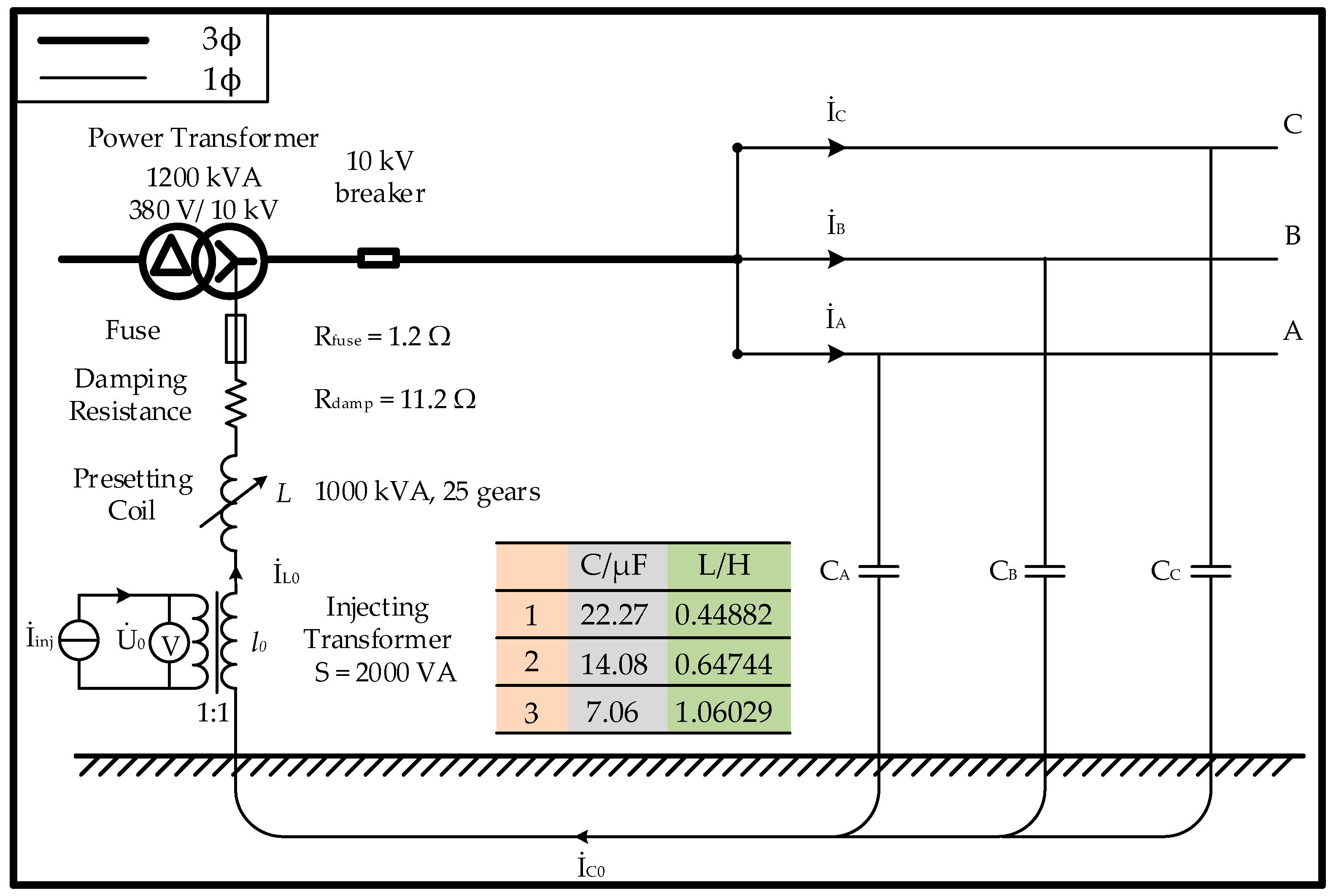
The signal injection of current signal of ISIM is conducted according to Figure 1. The low-voltage terminal of arc suppression coil L is connected in series with injecting transformer l0, whose turn ratio is 1:1, and the injecting current signal is injected into l0. Compared with the traditional injection pattern of current signal, the new injection pattern in this paper adapts the same topological structure. It could produce a higher amplitude current signal than other traditional injection pattern of current signal, which would enhance the performance of resisting external electromagnetic interference. Moreover, the new injection pattern is free from undergoing a higher amplitude of neutral-to-ground voltage, of which most of neutral-to-ground voltage is divided by coil. Furthermore, there is no longer risking switchgear explosion, caused by the short-circuit fault of the secondary side of the injecting transformer, to inject signal. Normally, the load of the system can be represented as a Y-connection impedance. The neutral point is ungrounded. Thus, the load is not taken into account in Figure 1. Besides, comparing with the impedance of line-to-ground capacitance, the system’s leakage resistances (RA & RB & RC) is so large that could be neglected. Assuming that line-to-ground capacitances are equal, which means CA = CB = CC. The equivalent circuit and its simplified circuit of zero sequence of Figure 1 are shown in Figure 2 based on the transformer Γ equivalent model. Moreover, constant frequency injection is utilized in measurement of line-to-ground capacitance according to Section 1.
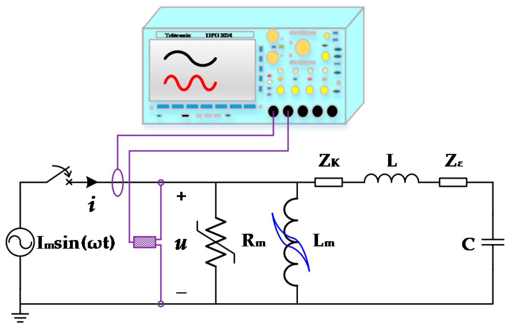
For the 1:1 turn ratio of the injecting transformer, all of the parameters shown in Figure 2 have no need to be referred. Zm represents transformer magnetizing impedance, Zm = Rm + j2πfLm. The magnetizing resistance Rm, whose value is affected by external voltage frequency f, represents the iron loss of the injecting transformer in the alternating magnetic field. Magnetizing inductance Lm also varies with external voltage frequency f. Z1σ and Z2σ is the primary impedance and the secondary impedance of l0, respectively. Let Zk = Z1σ + Z2σ, then Zk is the short-circuit impedance of l0. The value of Zk is known and linear to external voltage frequency f. The line stray impedance in zero sequence is represented by Zε, which is normally low, compared with line-to-ground impedance, which could be neglected. The line-to-ground capacitance, represent by C, is the aggregated value of the line-to-ground capacitance in each phase.
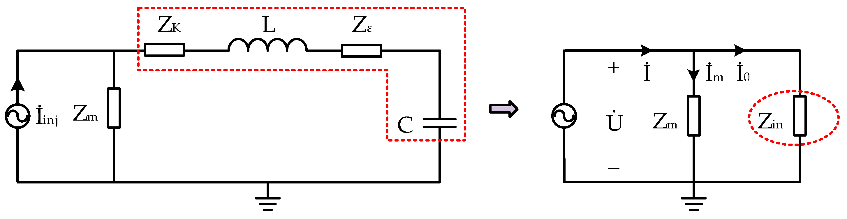
As shown in Figure 3, the current is injected into the secondary side of l0 and injecting port’s voltage is measured when launching the measurement. The ISIM is employed to measure line-to-ground capacitance C through vector information of the injecting port based on the known parameters (Zk & L) and the transformer magnetizing impedance Zm. Although operating the ISIM through the vector calculation method is simple, it has a higher demand for process module for its complex operation. Thus, the amplitude calculation method and the phase calculation method are derived and those validations are testified by experiment. It should be noted that the three calculation methods above have taken the magnetizing impedance into consideration. If the degree of simplification of magnetizing impedance is reduced, the measurement of line-to-ground capacitance is also simplified, which operates the calculation through the simplified model of magnetizing impedance rather than the improved model. For example, if the magnetizing impedance is treated as the ideal model (namely SIM), then operate the calculation with Zm = ∞, while treated as rated parameter model (namely RSIM), then operate the calculation with the rated magnetizing impedance.
Let: zero-sequence line resistance R0 = RL + Rk, zero-sequence line inductance L0 = L + Lk, zero-sequence line impedance Z0 = R0 + jωL0. Hence, input resistance Rin = R0, input impedance Xin = ωL0 − (ωC)−1.
2.1. Vector Calculation Method
The original injecting current is shunted by Zm, thus the current flow through Zin is:
So, the input impedance of load Z is:
Then, line-to-ground impedance ZRC is calculated by subtracting zero-sequence line impedance Z0 from Z:
Take the imaginary part of ZRC and divide by angular frequency ω to get the line-to-ground capacitance C:
This method is carried out through the vector information in injecting port, based on the known parameters, and takes magnetizing impedance’s frequency characteristic into consideration.
2.2. Amplitude Calculation Method
The admittance vector equation of the injecting port in Figure 3 can be calculated by:
Operating mod and square to both sides of Equation (6), then Equation (6) is deform as:
Let PRM = Rm/(Rm2 + Xm2), PXM = Xm/(Rm2 + Xm2). Once frequency is confirmed, Rm and Lm is assured, then PRM and PXM are constant values. Equation (7) can be rewritten as:
Derived from Equation (1), then we can get:
where Z02 = R02 + ω2L02, then put Equation (9) into Equation (8):
where A = M2Z02 − 2PRMR0 − 2PXMX0 − 1, B = PXM − M2X0. When there are two kinds of signals of different frequencies, they can be described as:
Then, C is given by:
This method operates calculation through two kinds of frequency signals’ voltage and current amplitude information in the injecting port and then calculates C through Equation (12), and also takes magnetizing impedance’s frequency characteristic into consideration.
2.3. Phase Calculation Method
The impedance vector equation of the injecting port in Figure 3 can be calculated by:
The tangent of impedance angle of the injecting port is given by:
Rewrite Equation (14),
Let K = PXM − PRMtanφ, which is a frequency-dependent parameter. Equation (15) can be rewritten as:
where W = KZ02 + X0 − R0tanφ, V = 2KX0 + 1, both of them vary with external frequency f. Similarly, they can be written as:
Then, C is calculated by:
This method utilizes two kinds of frequency signals’ voltage and current phase information in the injecting port, and then calculates C through Equation (18). The influence of magnetizing impedance is also considered in this method.
The three measurements of line-to-ground capacitance are shown above; it can be concluded that magnetizing impedance will influence the accuracy of measurement directly. In addition, the more saturated the iron core of the injecting transformer, the larger the deviation between calculation value and true value of magnetizing impedance, and the more affected the results. Besides, the injecting transformer in traditional measurement always owns a small capacity, which is prone to be saturated.
3. Experiment Platform and Techniques
3.1. Line-Ground-Capacitance Measurement
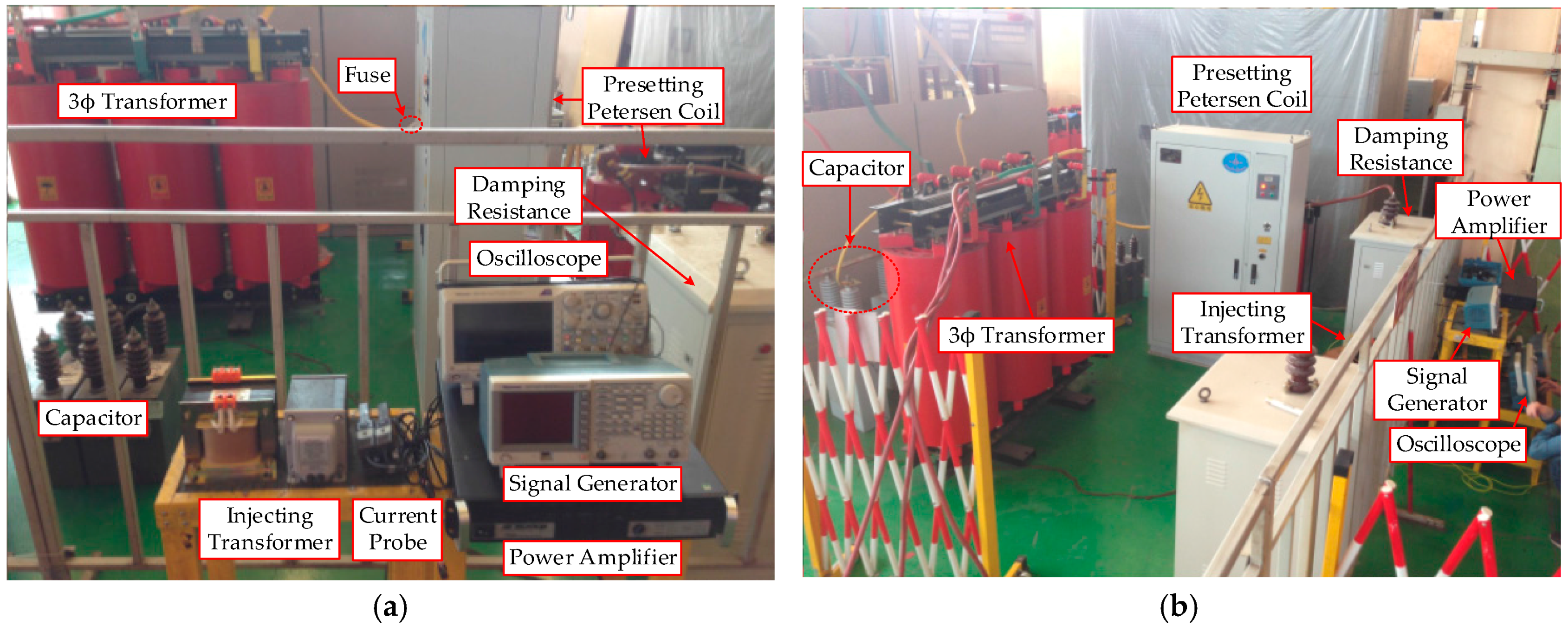
According to the diagram illustrated in Figure 1, the test circuit of 10 kV experiment platform is established as Figure 4, and its equipment and connection are shown in Figure 5.
Lumped parameter capacitors are applied to represent the line-to-ground capacitance C of the system. The capacitors are connected to the outlet terminal of a three-phase 380 V/10 kV transformer. The transformer is energized by applying 380 V voltage to the low voltage side. The resistance of fuse Rfuse is 1.2 Ω and it is in series with the neutral point to protect the coil. Once the capacitance C is changed via regulating the lumped capacitor’s value in each phase, the presetting arc suppression coil L will be adjusted to the vicinity of over-compensation, which is also near the resonant point. Thus, in this experiment, the parameter L varies with the changing of C. The coil is in series with the damping resistance (Rdamp = 11.2 Ω) to avoid zero-sequence circuit resonance. Damping resistance is connected to one endpoint of the primary side of l0. And another endpoint of the primary side of l0 is grounded. The turn ratio of l0 is 1:1, and the rated capacity is 2000 VA. When it works at the rated frequency, Rm = 467.5 Ω, Lm = 1.9558 H, Rk = 1.17 Ω, Lk =1.4 mH. Hence, the rated parameter model of the injecting transformer is obtained. Arbitrary function signal generator, TEKTRONIX AFG 3011 (TEKTRONIX, Beaverton, OR, USA), is applied to produce a sinusoidal signal. This signal is amplified by a power amplifier AE TECHRON 7224 (AE TECHRON, Elkhart, IN, USA), which turns the voltage signal into the current signal. And the gain of amplifier is adjustable. For the whole measurement, the root mean square (RMS) of the injecting current signal is no more than 1 A, and the injecting power is no more than 50 W. The input current signal is injected into the secondary side of l0 and the return voltage signal is also measured from the secondary side of l0. The signals of the input current and return voltage are sampled and filtered. Then the fast Fourier transform (FFT) and the calculation method are applied to achieve the final results. In order to strengthen the Electro Magnetic Compatibility (EMC) of the measuring system, the improved injection pattern is applied to the tests, which can mitigate the influence of the noise upon the current signal and have a high signal-to-noise ratio as the explanation in Section 1. Moreover, during the measurement, the data acquisition module of the measuring system is fine-grounded and the data is transferred through the coaxial cable whose shielding layer is grounded as well. Besides, the sampled signals of the input current and return voltage are filtered by a low-pass digital filter. In future work, the analog filter should be investigated for better EMC performance.
Besides, the line stray impedance Zε of transmission lines or cables could have little effect on the measurement of line-to-ground capacitance. However, the line stray impedance Zε is quite small compared with the line-to-ground impedance. Therefore, in most of the methods for line-to-ground capacitance measurement, the effect of the line stray impedance on the test results is normally ignored.
As mentioned in Section 2, the load of most of the systems in practice can be treated as a Y-connection impedance whose neutral points have not grounded. In this situation, the injecting zero-sequence current will not flow through the load, then the load has no influence upon the measurement. For a few special systems, its load can be simplified as a Y-connection impedance whose neutral point is grounded, but the load of the three phases is an approximate balance in formal. The zero-sequence current, flowing through the load, is quite small, which would also have little influence upon the measurement results. Thus, the presented method can be applied to the real power system.
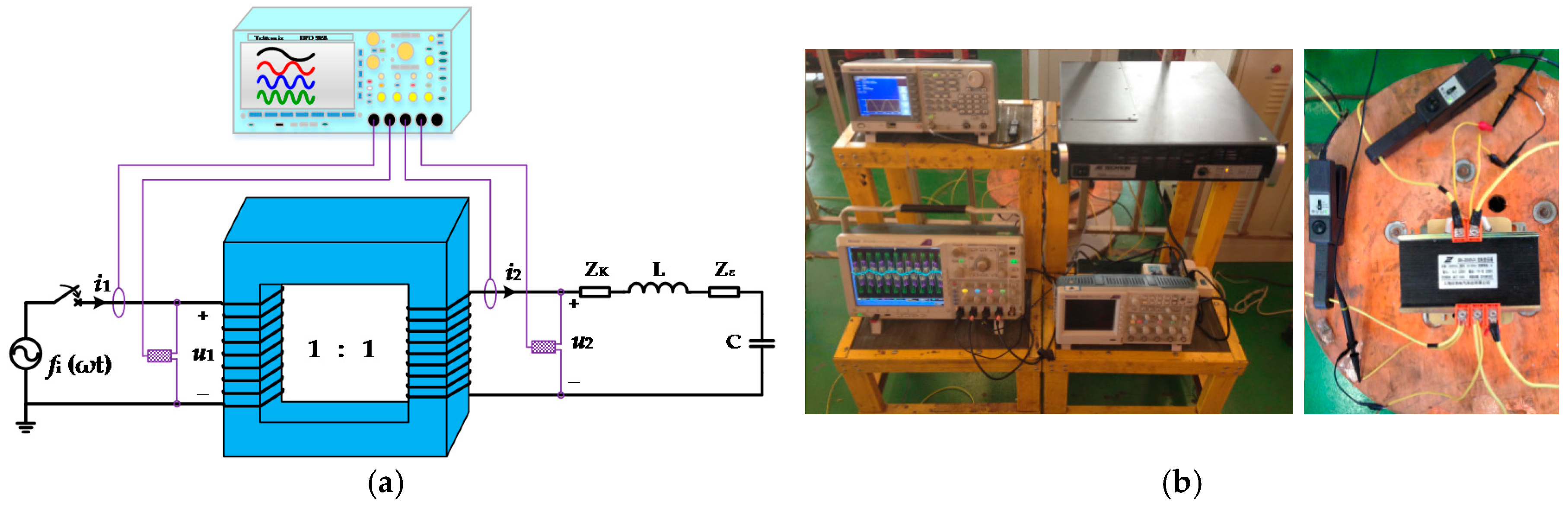
3.2. Magnetizing Impedance’s Frequency Characteristic Measurement
In the process of injecting current signal, it is found that the iron core of l0 is prone to be saturated when the frequency of injecting current signal is low. As shown in Figure 6, the frequency of injecting signal is 10 Hz, and injecting power is less than 50 W, which is much smaller compared to the injecting transformer rated capacity 2000 VA. But previous studies exclude the error caused by Zm, thus its recommended frequency groups have some randomness. Hence, it is necessary to measure the magnetizing impedance’s frequency characteristic to get an improved magnetizing impedance model for the calculation of line-to-ground capacitance, particularly when the injecting transformer is deeply saturated. It should be noted that the capacity of the power transformer is much higher than that of the injecting power. Hence, the saturation of the power transformer caused by the injecting power does not need to be considered.
The frequency scope of the injecting current signal is roughly 0–120 Hz [9,10,11,21,22]. Thus, the currents with eight frequency points, which is uniformly distributed in this frequency scope, are applied to the injecting transformer to obtain the frequency characteristic of the magnetizing impedance of the corresponding frequency based on the values of injecting current signal and returned voltage signal. During measurement of the frequency characteristic of magnetizing impedance, l0 is put into zero-sequence circuit, which assures that the circuit is the same as that of the line-to-ground capacitance measurement. Besides, the system does not need to be energized in the process of this measurement, because l0 is in series with L, which is a large inductance, and the voltage of l0 is always low. Then, the calculation of magnetizing impedance at those frequency points is operated. The formula to calculate magnetizing impedance under load is:
The diagram and physical photo of measurement are shown in Figure 7.
4. Experiment Results and Analysis
Experiment platform is established and its test circuit is shown in Figure 8. According to Figure 4, when C is set as 22.27 μF and 14.08 μF and 7.06 μF, the corresponding inductance of coil is regulated to 0.44882 H and 0.64744 H and 1.06029 H. Then, eight different current signals are injected into zero-sequence circuit in eight times, respectively. The results of vector calculation method show that the calculation of C based on ISIM is prior to the calculation based on SIM and RSIM. Moreover, the results of vector calculation method based on ISIM are excellent in the range of 10–100 Hz. Thus, six two-frequency groups are chosen in that scope to operate amplitude and phase calculation based on ISIM.
4.1. Vector Calculation Method Results
The results of the vector calculation method, based on different magnetizing impedance models, are shown in Table 1. C is the sum of capacitance of lumped capacitors in the system, while L is the corresponding inductance value of the presetting arc suppression coil. Cf is the calculation result based on ISIM, and the relative error is ef. C50Hz is the calculation result based on RSIM, and the relative error is e50Hz. C0 is the calculation result based on SIM, and the relative error is e0.
As shown in Table 1, it can be concluded that:
- (1).
- Cf is more accurate than C50Hz, while C50Hz is more accurate than C0.
- (2).
- If the calculation is based on SIM, the recommended frequency scope of the injecting signal should be in the vicinity of the rated frequency.
- (3).
- If the calculation is based on RSIM, the recommended frequency scope of the injecting signal should be 30~80 Hz, but the results are not stable and could be affected by the external topology and frequency.
- (4).
- If the calculation is based on ISIM, the recommended frequency scope could reach 20~120 Hz, and the results are more stable and reliable.
- (5).
- With the rise of frequency f of the injecting signal, e50Hz and e0 decrease first and then increase:
- when f is low, the iron core is more vulnerable to be saturated, thus magnetizing impedance for calculation far away from the true value;
- when f is high, the impedance of line-to-ground capacitance is low, and the line stray impedance Zε in zero sequence is high. Thus, calculation error and system error increase during calculation.
- (6).
- With the rise of frequency f of the injecting signal, ef has the same tendency, but the tendency is not obvious because of the improvement caused by considering the magnetizing impedance’s frequency characteristic in the ISIM calculation.
4.2. Amplitude Calculation Method Results
Based on the results in Section 4.1, six two-frequency groups are chosen and each group contains two frequencies: (10, 20), (20, 40), (30, 60), (40, 60), (40, 80), (40, 100). Moreover, amplitude information of voltage and current is employed in Section 4.1 to operate the calculation through amplitude calculation method based on ISIM.
The results are shown in Table 2. The two-frequency group consists of f1 and f2. The results of amplitude calculation is Cmf, and emf represents its relative error.
Firstly, it is obvious that the injecting signal group (10, 20) produces low precision, which is caused by iron core saturated at low frequency. The magnetic flux Φ ≈ U/(4.44Nf), where U is external voltage and N is the number of turns of l0. The larger the magnetic flux Φ, the deeper the saturation of the iron core [3,25]. Thus, the degree of saturation of the iron core is subject to the influence of external voltage U when the external frequency f is low. Therefore, the frequency component of two-frequency of injecting current signal should not be too low. Secondly, the line stray impedance Zε cannot be ignored when the injecting signal group (40, 100) is utilized. Besides, the calculation error, caused by the decrease of magnitude of line-to-ground impedance, is introduced into the results when frequency is high. Therefore, the frequency component of two-frequency of the injecting signal frequency should be properly selected. The recommend frequency scope for amplitude calculation method is 20–80 Hz.
4.3. Phase Calculation Method Results
The calculation is operated as Section 4.2, and phase information of voltage and current in Section 4.1 is employed. The results are shown in Table 3. The results calculated by phase calculation method is Cpf, and epf represents its relative error. Compared with Table 2, the suitable frequency scope of phase calculation method is much narrower, and distributes around the rated frequency. The reason is that compared with amplitude information, phase information of electrical signal is more vulnerable to the influence of electromagnetic interference. Therefore, in order to assure the accuracy of phase calculation results, it is necessary to apply shielding measures in the measurement process.
5. Conclusions
An ISIM to measure line-to-ground capacitance is proposed, and its validation is investigated. The ISIM is operated through vector information, amplitude information and phase information of the injecting port. The results are concluded as follows:
- (1).
- The topology of zero sequence of ISIM is similar to traditional methods and its applied frequency scope is extended and the accuracy of calculation is improved.
- (2).
- The saturation of iron core at low frequency and the system error due to line stray impedance Zε in zero sequence at high frequency are the major causes of measurement error.
- (3).
- When the injecting transformer is a transformer of small capacity, it is necessary to measure the frequency characteristic of magnetizing impedance for better results.
- (4).
- The frequency group should be selected in the range of 20–80 Hz, if line-to-ground capacitance is calculated through amplitude calculation method and phase calculation method via two-frequency information.
- (5).
- Nice shielding and filtering are demanded to obtain reasonable results via phase calculation method, because electrical signal is more vulnerable to the influence of electromagnetic interference.
Acknowledgments
This work is supported by the National Natural Science Foundation of China (51477018 and 51177182), and the Funds for Innovative Research Groups of China (51321063).
Author Contributions
Qing Yang contributed to the research idea and theoretical analysis of line-to-ground capacitance measurement. Bo Zhang conceived and designed the experiments, and drafted the manuscript. Jiaquan Ran checked the design of the experiment and gave valuable advice, Song Chen, Yanxiao He and Jian Sun worked on data analysis.
Conflicts of Interest
The authors declare no conflict of interest.
References
- Zadeh, M.R.D.; Sanaye-Pasand, M.; Kadivar, A. Investigation of neutral reactor performance in reducing secondary arc current. IEEE Trans. Power Deliv. 2008, 23, 2472–2479. [Google Scholar] [CrossRef]
- Wang, J.; Yang, Q.; Sima, W.X.; Yuan, T.; Zahn, M.K. A smart online over-voltage monitoring and identification system. Energies 2011, 4, 599–615. [Google Scholar] [CrossRef]
- Chen, L.; Yang, Q.; Wang, J.; Sima, W.X.; Yuan, T. Classification of fundamental ferroresonance, single phase-to-ground and wire breakage over-voltages in isolated neutral networks. Energies 2011, 4, 1301–1320. [Google Scholar] [CrossRef]
- Amin, M. A smart self-healing grid: In pursuit of a more reliable and resilient system [in my view]. IEEE Power Energy Mag. 2014, 12, 110–112. [Google Scholar] [CrossRef]
- Simpson-Porco, J.W.; Bullo, F. Distributed monitoring of voltage collapse sensitivity indices. IEEE Trans. Smart Grid 2016, 7, 1–10. [Google Scholar] [CrossRef]
- Taniguchi, T.; Kaisaki, K.; Fukui, Y. Automated linear function submission-based double auction as bottom-up real-time pricing in a regional prosumers’ electricity network. Energies 2015, 8, 7381–7406. [Google Scholar] [CrossRef]
- Cho, J.; Kim, J.H.; Lee, H.J. Development and improvement of an intelligent cable monitoring system for underground distribution networks using distributed temperature sensing. Energies 2014, 7, 1076–1094. [Google Scholar] [CrossRef]
- Kang, H.K.; Chung, I.Y.; Moon, S.I. Voltage control method using distributed generators based on a multi-agent system. Energies 2015, 8, 14009–14025. [Google Scholar] [CrossRef]
- Zeng, X.; Xu, Y.; Wang, Y. Some novel techniques for insulation parameters measurement and petersen-coil control in distribution systems. IEEE Trans. Ind. Electron. 2010, 57, 1445–1451. [Google Scholar] [CrossRef]
- Yao, H. The Resonance Grounding of the Electric System, 2nd ed.; China Electronic Power Press: Beijing, China, 2001. (In Chinese) [Google Scholar]
- Griffel, D.; Harmand, Y. A new deal for safety and quality on MV networks. IEEE Trans. Power Deliv. 1997, 12, 1428–1433. [Google Scholar] [CrossRef]
- IEEE Recommended Practice for Grounding of Industrial and Commercial Power Systems; IEEE Std. 142-2007 (Revision of IEEE Std. 142-1991); IEEE: New York, NY, USA, 2007.
- Baranski, M.; Decner, A.; Polak, A. Selected diagnostic methods of electrical machines operating in industrial conditions. IEEE Trans. Dielectric. Electr. Insul. 2014, 21, 2047–2054. [Google Scholar] [CrossRef]
- Meng, X.; Tai, N.L.; Hu, Y.; Yang, X. Shunt Petersen-coil with resistor for single phase fault detection in resonant grounded power distribution systems. Adv. Mater. Res. 2013, 860–863, 2007–2012. [Google Scholar] [CrossRef]
- Suonan, J.L.; Yang, C.; Yang, Z.L.; Song, G.B. Study of time-domain compensation algorithm of capacitive current for parallel transmission lines protection. Proc. CSEE 2010, 30, 77–81. (In Chinese) [Google Scholar]
- Zeng, X.; Hu, J.Y.; Wang, Y.; Xiong, T. Suppressing method of three-phase unbalanced overvoltage based on distribution networks flexible grounding control. Proc. CSEE 2014, 34, 678–684. (In Chinese) [Google Scholar]
- Lian, H.B.; Yang, Y.H.; Tan, P.W.; Qu, Y.L.; Qi, Z. Analysis on measuring error of capacitance current in medium-voltgae power network by biased capacitance method. Power Syst. Technol. 2005, 29, 54–58. (In Chinese) [Google Scholar]
- Yan, X.; He, Z.; Chen, W. An investigation into arc self-extinguishing characteristics on Peterson coil compensated system. In Proceedings of the International Conference on High Voltage Engineering and Application, Chongqing, China, 9–13 November 2008. [Google Scholar]
- Wu, J. Capacitive current measurement methods for arc-suppression coil with automatic tuning. Int. J. Digit. Content Technol. Its Appl. 2012, 6, 625–633. [Google Scholar]
- Li, W.; Chen, J.; Jiang, M.; Hu, Z.J.; Cheng, X. Setting of zero-sequence current compensation coefficient for ground distance relays of double-circuit transmission lines on same tower considering capacitive current. Power Syst. Technol. 2012, 36, 281–284. (In Chinese) [Google Scholar]
- Liu, L.; Sun, J. A new method to measure capacitive current in distribution network. Power Syst. Technol. 2001, 25, 63–65. (In Chinese) [Google Scholar]
- Zeng, X.; Xu, Y.; Chen, B.; Zhang, P.; Yuan, C. A novel measuring method of capacitive current for insulated neutral distribution networks. Autom. Electr. Power Syst. 2009, 33, 78–81. (In Chinese) [Google Scholar]
- Avila-Montes, J.; Campos-Gaona, D.; Vázquez, E.M.; Rodríguez-Rodríguez, J.R. A Novel compensation scheme based on a virtual air gap variable reactor for AC voltage control. IEEE Trans. Ind. Electron. 2014, 61, 6547–6555. [Google Scholar] [CrossRef]
- Tian, M.; Li, Q.; Li, Q. A controllable reactor of transformer type. IEEE Trans. Power Del. 2004, 19, 1718–1726. [Google Scholar] [CrossRef]
- Chen, X.; Chen, B.; Tian, C.; Yuan, J. Modeling and harmonic optimization of a two-stage saturable magnetically controlled reactor for an arc suppression coil. IEEE Trans. Ind. Electron. 2012, 59, 2824–2831. [Google Scholar] [CrossRef]
- Luo, A.; Shuai, Z.; Zhu, W.; Shen, Z.J. Combined system for harmonic suppression and reactive power compensation. IEEE Trans. Ind. Electron. 2009, 56, 418–428. [Google Scholar] [CrossRef]
- Kumar, C.; Mishra, M.K. An improved hybrid DSTATCOM topology to compensate reactive and nonlinear loads. IEEE Trans. Ind. Electron. 2014, 61, 6517–6527. [Google Scholar] [CrossRef]
- Zivanovic, R.; Schegner, P.; Seifert, O.; Pilz, G. Identification of the resonant-grounded system parameters by evaluating fault measurement records. IEEE Trans. Power Deliv. 2004, 19, 1085–1090. [Google Scholar] [CrossRef]
- Schulze, R.; Schegner, P.; Zivanovic, R. Parameter identification of unsymmetrical transmission lines using fault records obtained from protective relays. IEEE Trans. Power Deliv. 2011, 26, 1265–1272. [Google Scholar] [CrossRef]
Figure 1.
Line-to-ground capacitance measurement.
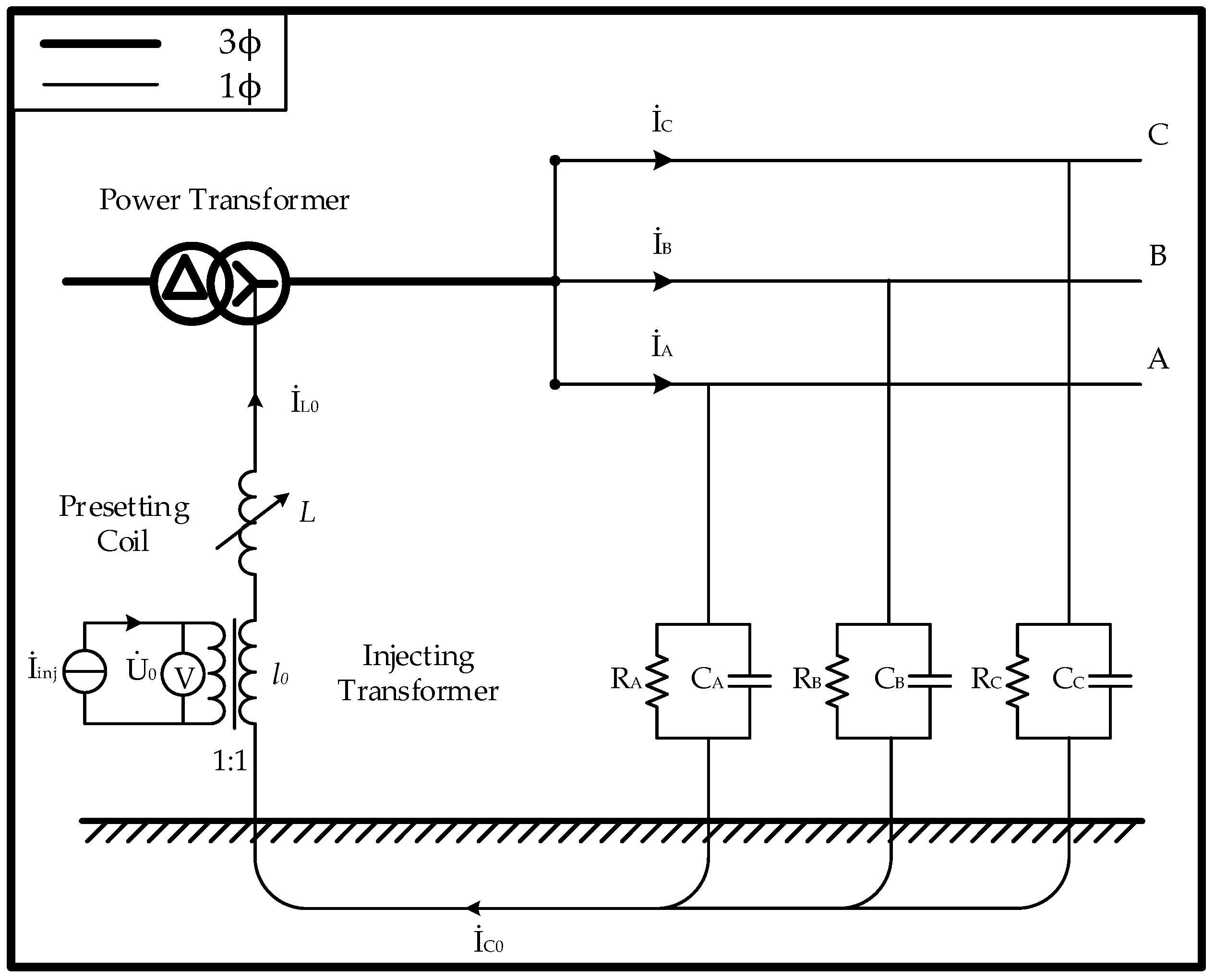
Figure 2.
Equivalent circuit. (a) Based on transformer Γ equivalent model; (b) Simplified equivalent circuit (Zk = Z1σ + Z2σ).
Figure 2.
Equivalent circuit. (a) Based on transformer Γ equivalent model; (b) Simplified equivalent circuit (Zk = Z1σ + Z2σ).
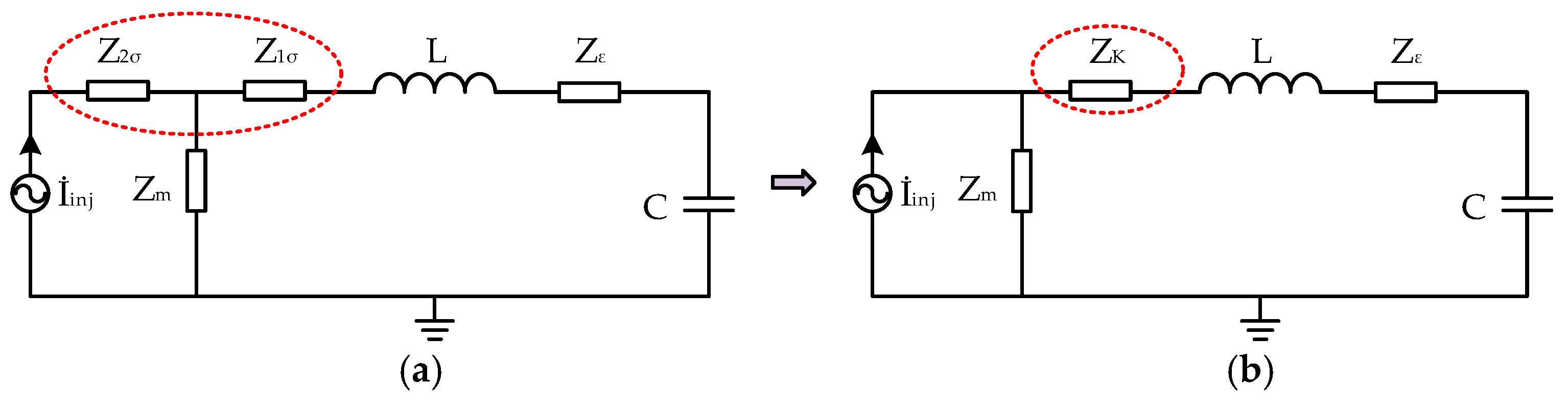
Figure 3.
Turn the impedance at right side of Zm into Zin.

Figure 4.
The test circuit of 10 kV experiment platform.

Figure 5.
The 10 kV experiment platform. (a) Equipment; (b) Connection of equipment in laboratory.

Figure 6.
The saturated phenomenon in secondary side of injecting transformer at 10 Hz injecting situation.
Figure 6.
The saturated phenomenon in secondary side of injecting transformer at 10 Hz injecting situation.
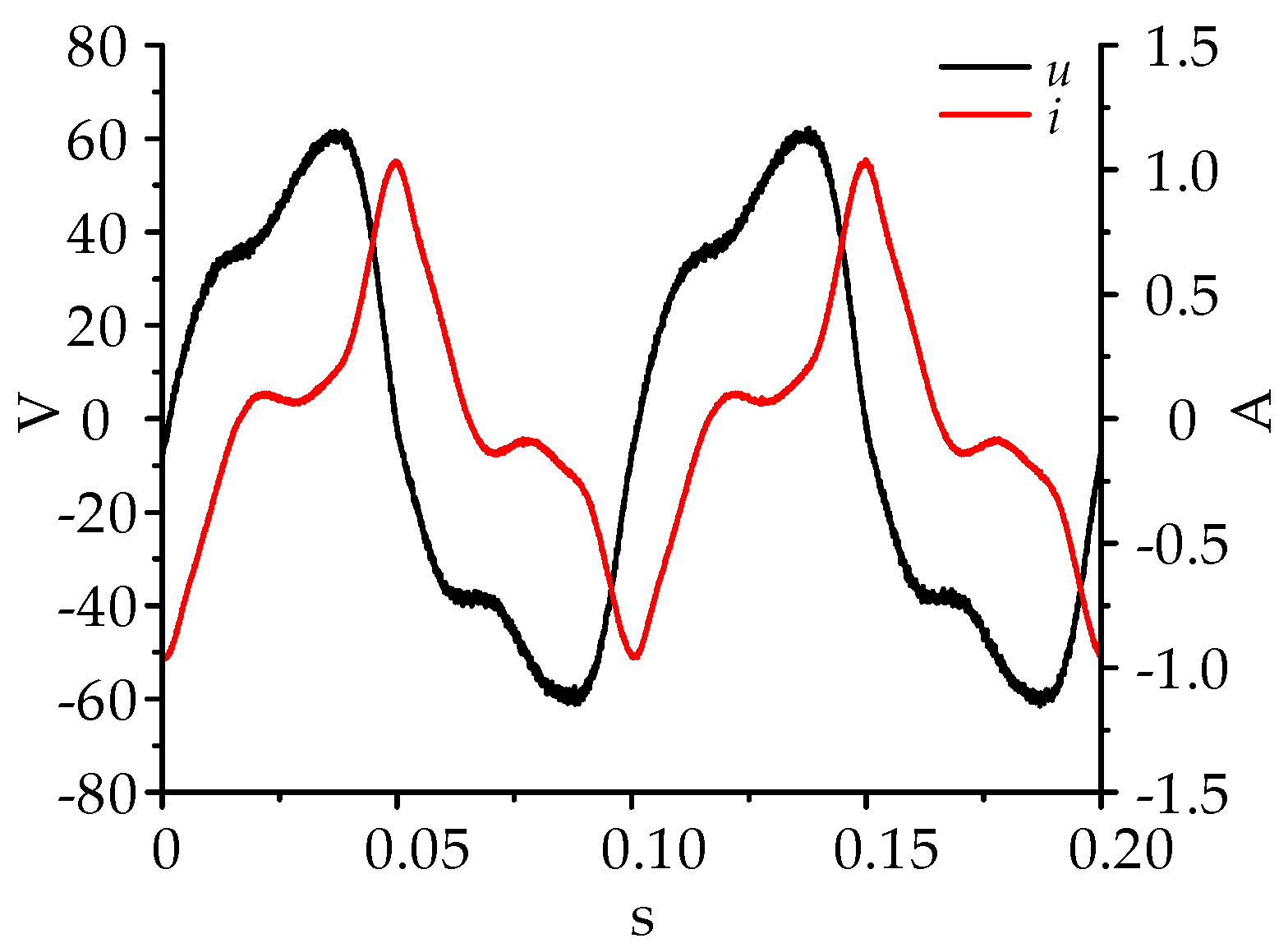
Figure 7.
Magnetizing impedance measurement. (a) Test circuit of magnetizing impedance measurement; (b) Laboratory setup.
Figure 7.
Magnetizing impedance measurement. (a) Test circuit of magnetizing impedance measurement; (b) Laboratory setup.

Figure 8.
Test circuit of zero sequence in experiment.


Table 1.
Vector calculation results based on different magnetizing impedance models.
| C (μF) | L (H) | f (Hz) | Calculation Capacitance (μF) | Relative Error (%) | ||||
|---|---|---|---|---|---|---|---|---|
| Cf | C50Hz | C0 | ef | e50Hz | e0 | |||
| 22.27 | 0.44882 | 10 | 20.96 | −171.26 | −193.28 | 5.88 | 869.02 | 967.89 |
| 20 | 21.43 | 17.63 | 13.24 | 3.77 | 20.84 | 40.55 | ||
| 30 | 22.37 | 21.69 | 19.98 | 0.45 | 2.6 | 10.28 | ||
| 40 | 22.43 | 22.74 | 21.39 | 0.72 | 2.11 | 3.95 | ||
| 60 | 22.33 | 22.57 | 21.69 | 0.27 | 1.35 | 2.6 | ||
| 80 | 21.69 | 21.52 | 18.47 | 2.6 | 3.37 | 17.06 | ||
| 100 | 19.31 | 21.07 | 16.31 | 13.29 | 5.39 | 26.76 | ||
| 120 | 24.45 | 15.88 | 11.02 | 9.79 | 28.69 | 50.52 | ||
| 14.08 | 0.64744 | 10 | 13.81 | −34.93 | −40.12 | 1.92 | 348.08 | 384.94 |
| 20 | 13.92 | 5.00 | −2.28 | 1.14 | 64.49 | 116.19 | ||
| 30 | 14.15 | 11.82 | 9.52 | 0.5 | 16.05 | 32.39 | ||
| 40 | 13.98 | 13.33 | 12.69 | 0.71 | 5.33 | 9.87 | ||
| 60 | 13.96 | 13.64 | 14.42 | 0.85 | 3.13 | 2.41 | ||
| 80 | 13.31 | 12.15 | 11.7 | 5.47 | 13.71 | 16.9 | ||
| 100 | 12.87 | 9.67 | 9.39 | 8.59 | 31.32 | 33.31 | ||
| 120 | 10.14 | 7.03 | 5.56 | 27.98 | 50.07 | 60.51 | ||
| 7.06 | 1.06029 | 10 | 5.85 | −123.84 | −211.76 | 17.14 | 1854.11 | 3099.43 |
| 20 | 6.98 | −0.02 | −5.53 | 1.13 | 100.28 | 178.33 | ||
| 30 | 7.14 | 6.22 | 3.33 | 1.13 | 11.9 | 52.83 | ||
| 40 | 7.11 | 6.51 | 5.43 | 0.71 | 7.79 | 23.09 | ||
| 60 | 6.93 | 6.92 | 6.92 | 1.84 | 1.98 | 1.98 | ||
| 80 | 6.90 | 6.15 | 5.54 | 2.27 | 12.89 | 21.53 | ||
| 100 | 7.30 | 5.15 | 4.09 | 3.4 | 27.05 | 42.07 | ||
| 120 | 6.93 | 3.95 | 3.01 | 1.84 | 44.05 | 57.37 | ||
Table 2.
Amplitude calculation results of ISIM in different capacitance.
| C (μF) | f1 (Hz) | f2 (Hz) | Cmf (μF) | emf (%) |
|---|---|---|---|---|
| 22.27 | 10 | 20 | 19.22 | 13.7 |
| 20 | 40 | 23.23 | 4.31 | |
| 30 | 60 | 23.99 | 7.72 | |
| 40 | 60 | 22.76 | 2.2 | |
| 40 | 80 | 22.59 | 1.44 | |
| 40 | 100 | 22.76 | 2.20 | |
| 14.08 | 10 | 20 | 16.96 | 20.45 |
| 20 | 40 | 13.42 | 4.69 | |
| 30 | 60 | 12.98 | 7.81 | |
| 40 | 60 | 14.02 | 0.43 | |
| 40 | 80 | 13.79 | 2.06 | |
| 40 | 100 | 13.70 | 2.70 | |
| 7.06 | 10 | 20 | 6.42 | 9.07 |
| 20 | 40 | 6.71 | 4.96 | |
| 30 | 60 | 6.94 | 1.70 | |
| 40 | 60 | 6.97 | 1.27 | |
| 40 | 80 | 6.88 | 2.55 | |
| 40 | 100 | 7.50 | 6.23 |
Table 3.
Phase calculation results of ISIM in different capacitance.
| C (μF) | f1 (Hz) | f2 (Hz) | Cpf (μF) | epf (%) |
|---|---|---|---|---|
| 22.27 | 10 | 20 | 19.46 | 12.62 |
| 20 | 40 | 21.87 | 1.80 | |
| 30 | 60 | 21.95 | 1.44 | |
| 40 | 60 | 22.28 | 0.04 | |
| 40 | 80 | 22.06 | 0.94 | |
| 40 | 100 | 23.4 | 5.07 | |
| 14.08 | 10 | 20 | 15.37 | 9.16 |
| 20 | 40 | 12.43 | 11.72 | |
| 30 | 60 | 12.44 | 11.65 | |
| 40 | 60 | 13.74 | 2.41 | |
| 40 | 80 | 12.33 | 12.43 | |
| 40 | 100 | 11.24 | 20.17 | |
| 7.06 | 10 | 20 | 7.68 | 8.78 |
| 20 | 40 | 6.52 | 7.65 | |
| 30 | 60 | 6.59 | 6.66 | |
| 40 | 60 | 7.29 | 3.26 | |
| 40 | 80 | 7.66 | 8.50 | |
| 40 | 100 | 6.26 | 11.33 |
© 2017 by the authors. Licensee MDPI, Basel, Switzerland. This article is an open access article distributed under the terms and conditions of the Creative Commons Attribution (CC BY) license (http://creativecommons.org/licenses/by/4.0/).
Share and Cite
MDPI and ACS Style
Yang, Q.; Zhang, B.; Ran, J.; Chen, S.; He, Y.; Sun, J. Measurement of Line-to-Ground Capacitance in Distribution Network Considering Magnetizing Impedance’s Frequency Characteristic. Energies 2017, 10, 477. https://doi.org/10.3390/en10040477
AMA Style
Yang Q, Zhang B, Ran J, Chen S, He Y, Sun J. Measurement of Line-to-Ground Capacitance in Distribution Network Considering Magnetizing Impedance’s Frequency Characteristic. Energies. 2017; 10(4):477. https://doi.org/10.3390/en10040477
Chicago/Turabian StyleYang, Qing, Bo Zhang, Jiaquan Ran, Song Chen, Yanxiao He, and Jian Sun. 2017. "Measurement of Line-to-Ground Capacitance in Distribution Network Considering Magnetizing Impedance’s Frequency Characteristic" Energies 10, no. 4: 477. https://doi.org/10.3390/en10040477
Note that from the first issue of 2016, this journal uses article numbers instead of page numbers. See further details here.