Limitations and Constraints of Eddy-Current Loss Models for Interior Permanent-Magnet Motors with Fractional-Slot Concentrated Windings

Abstract
:1. Introduction
Contributions and Outline of the Paper
2. Review of Eddy-Current Loss Models
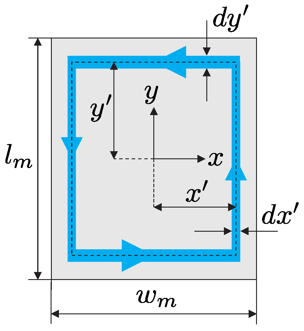
2.1. Model A: Assumed Eddy-Current Paths
2.2. Model B: Solving the Helmholtz Equation with the Imposed Source Term
2.3. Model C: Solving the Helmholtz Equation Prescribing Boundary Surface Currents
3. Analysis and Evaluation
3.1. Loss-Model Constraints When Applied to IPMs
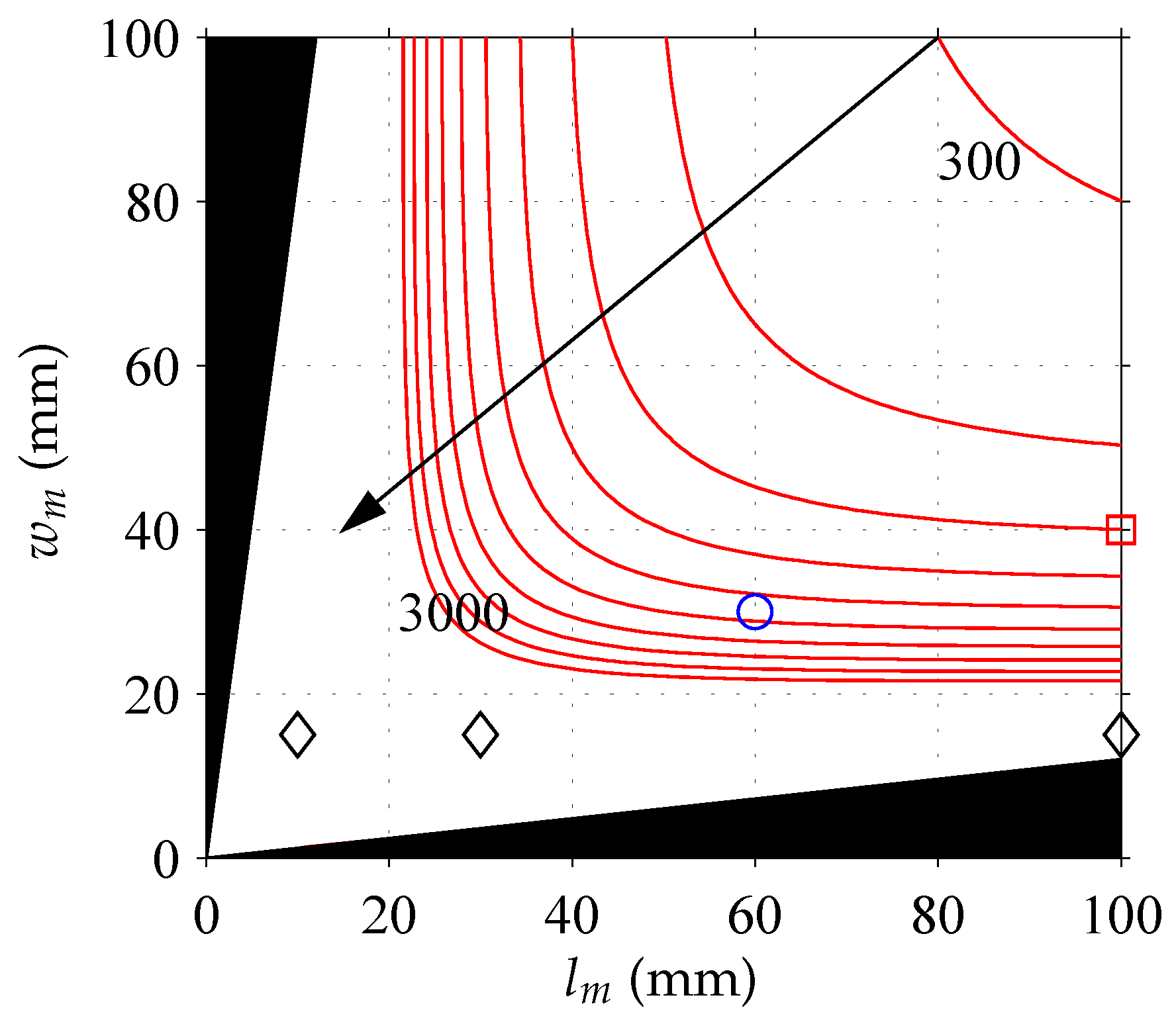
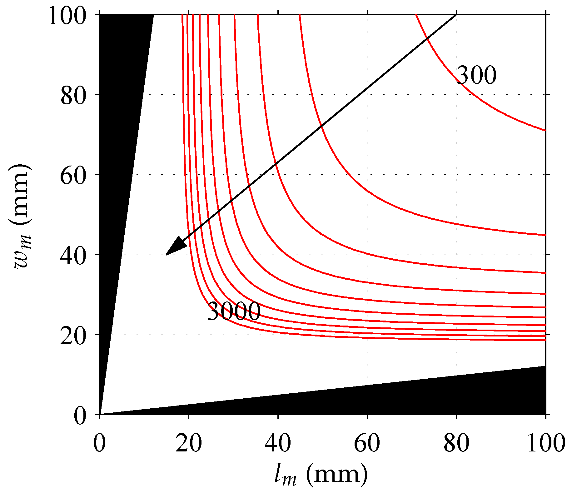
3.2. Limits for Model A Due to Eddy-Current Reaction Fields
Approximation of
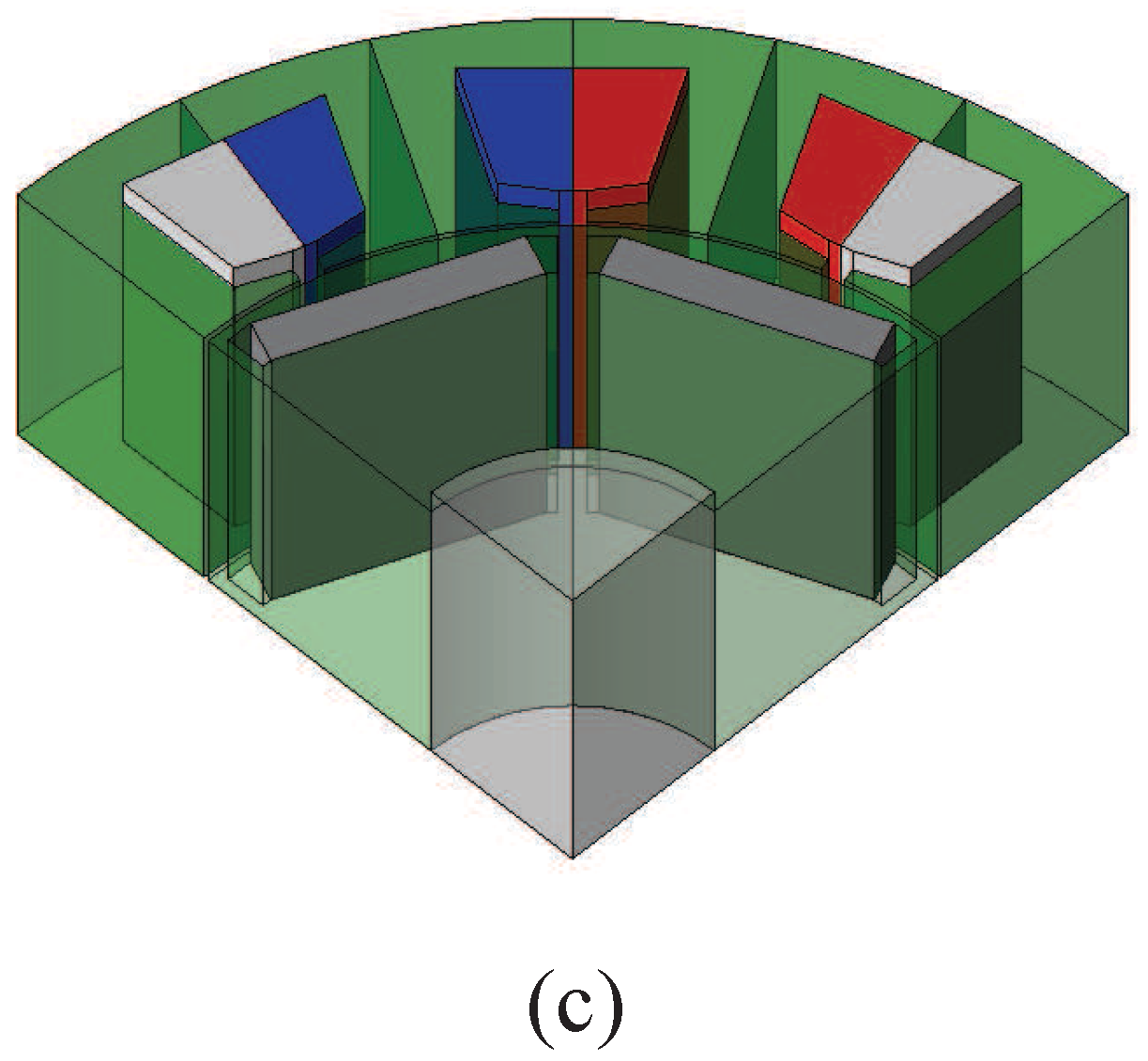
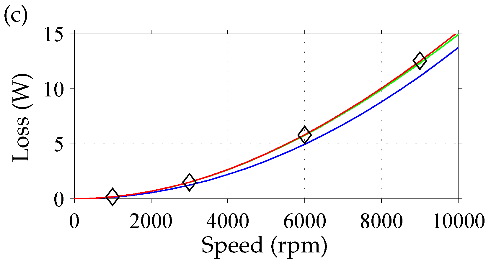
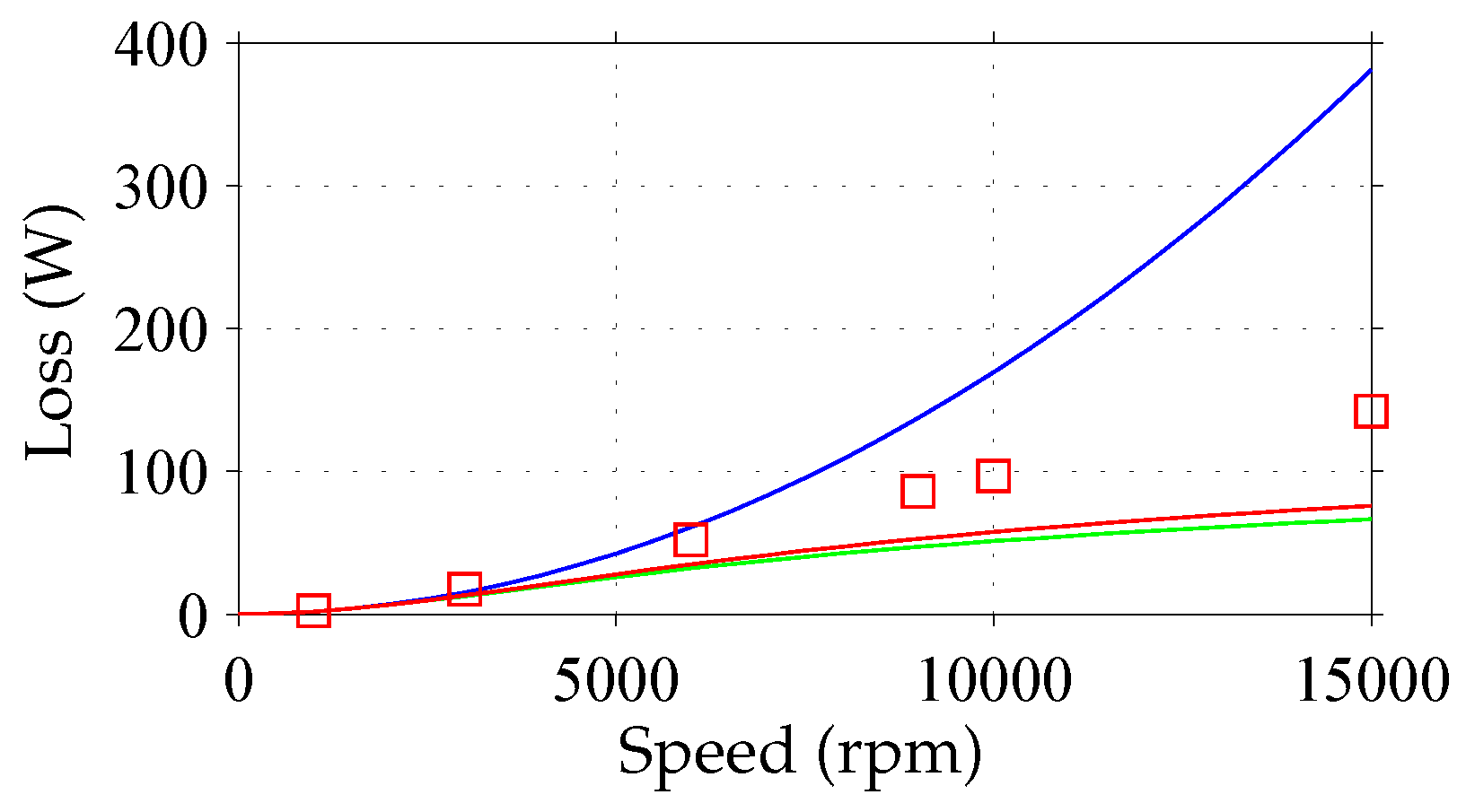
3.3. 3DFEM-Evaluation
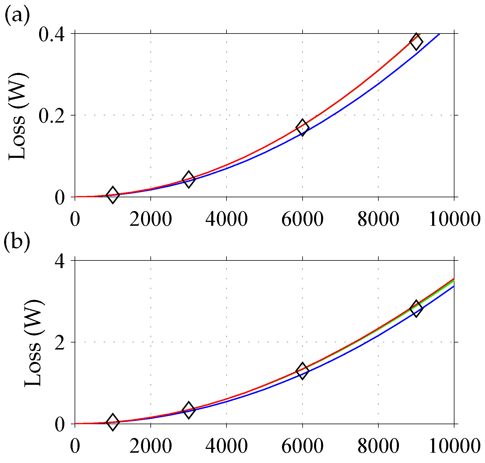
3.3.1. Negligible Eddy-Current Reaction Fields
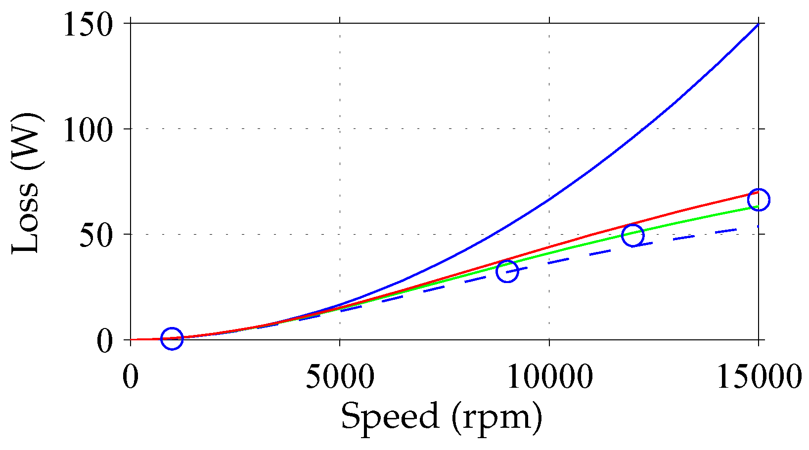
3.3.2. Non-Negligible Eddy-Current Reaction Fields
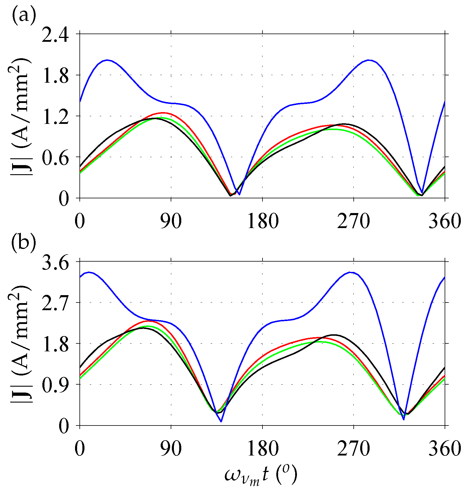
3.3.3. Impact of Non-Uniform Flux-Density Variation
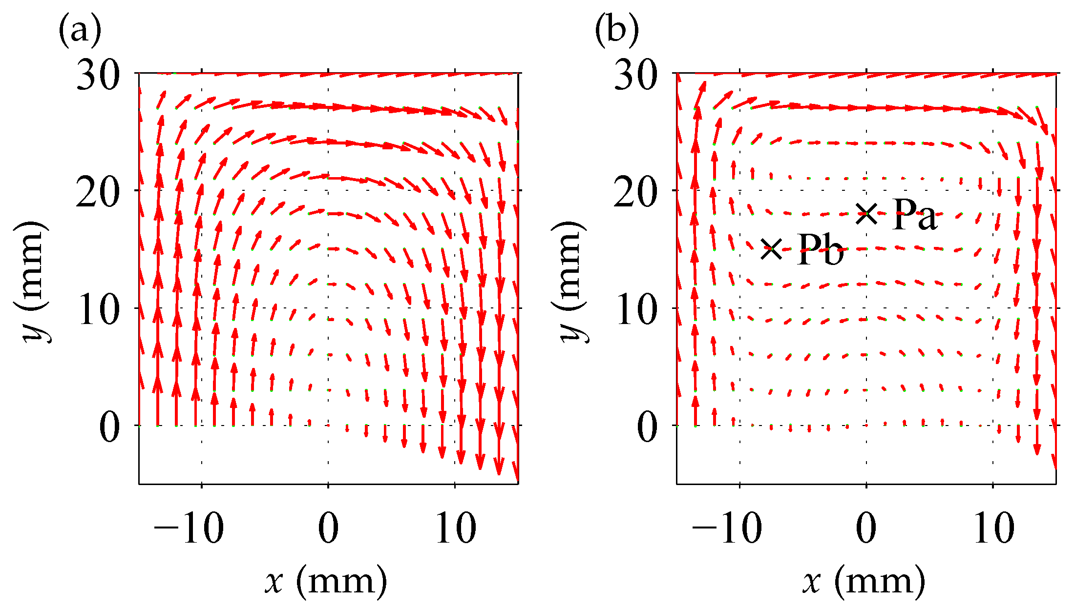
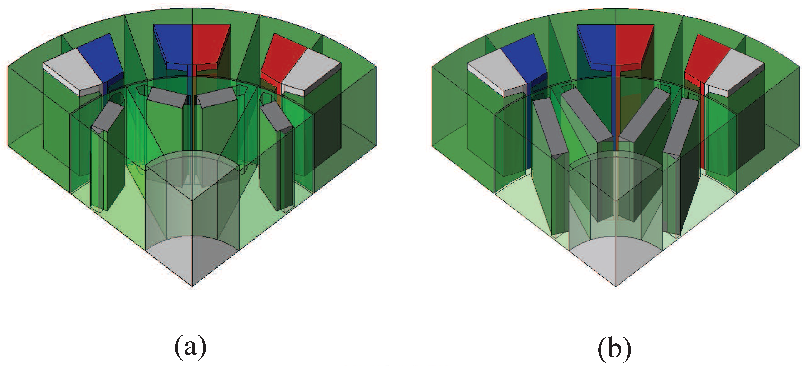
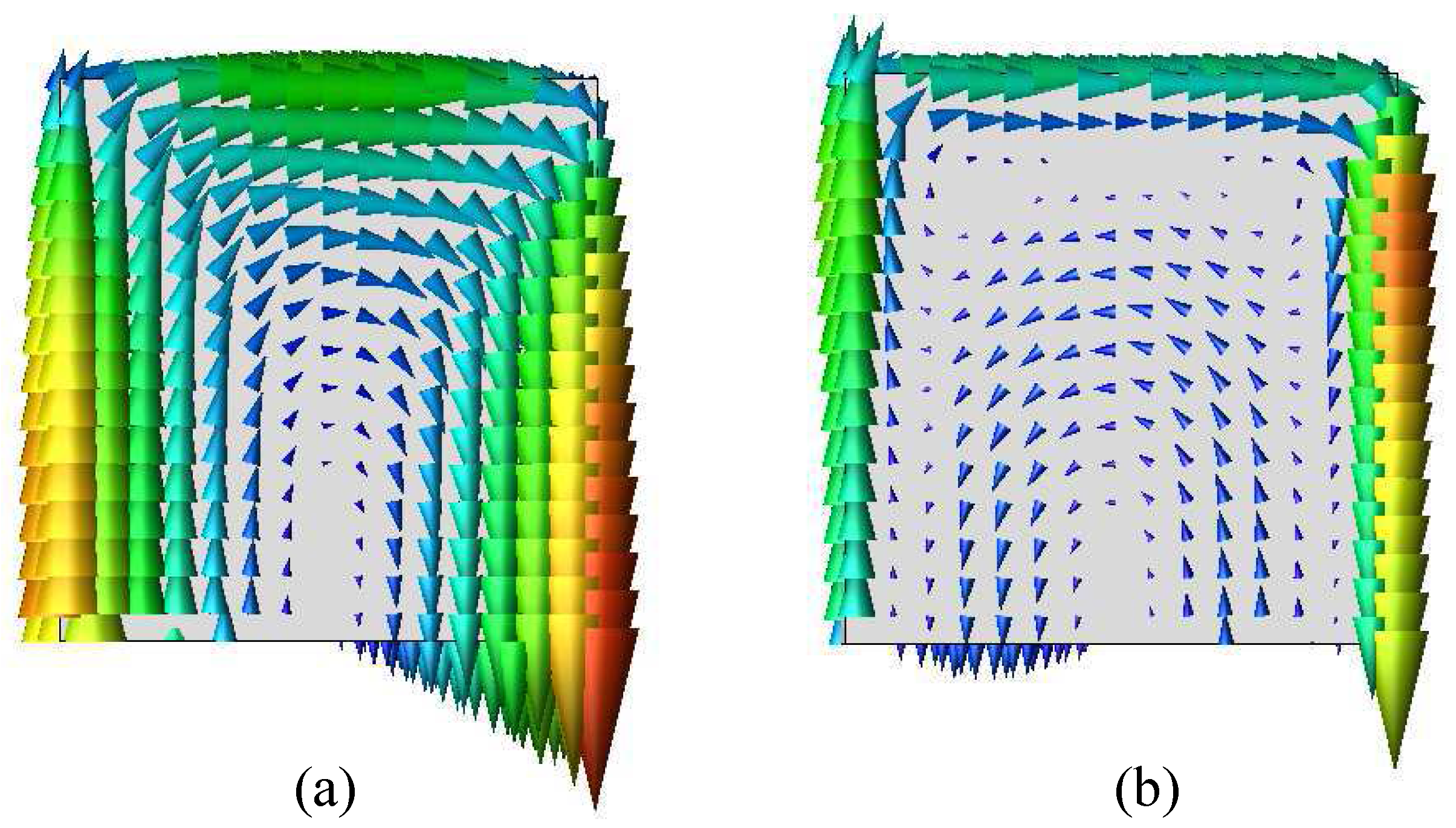
3.4. Visualization of the Resulting Eddy-Current Distribution
4. PM Losses in Automotive Applications
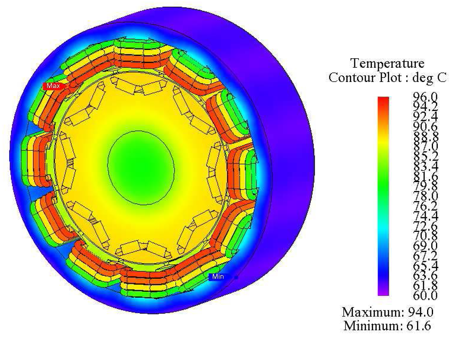
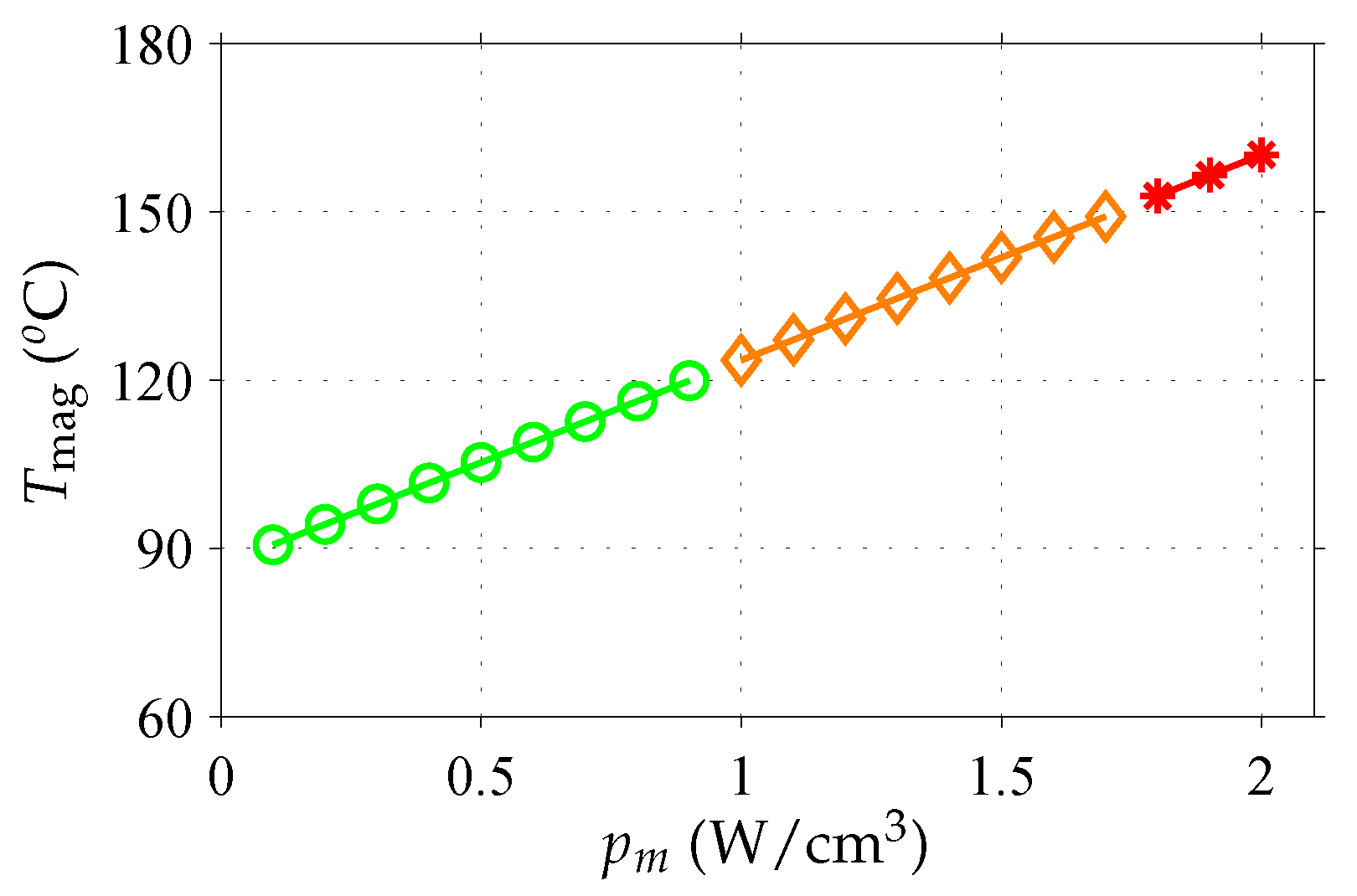
4.1. Thermal Impact
4.2. Losses for p and Common in Automotive Applications
5. Conclusions
Acknowledgments
Author Contributions
Conflicts of Interest
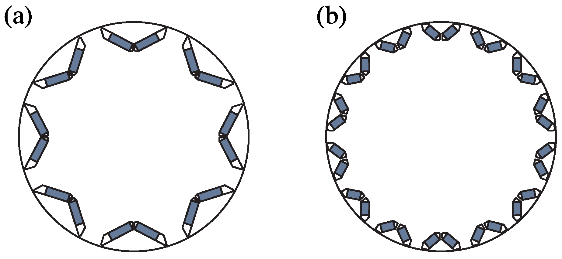
Appendix A. FSCW Fundamentals
Appendix A.1. Preliminaries
Appendix A.2. Air-Gap MMF Distribution Due to Stator Current
Appendix A.3. Winding Factor for Harmonic ν
Appendix A.4. PM Flux Density Variations
Appendix B. IPM Parameters

| Parameter | Value | Unit |
|---|---|---|
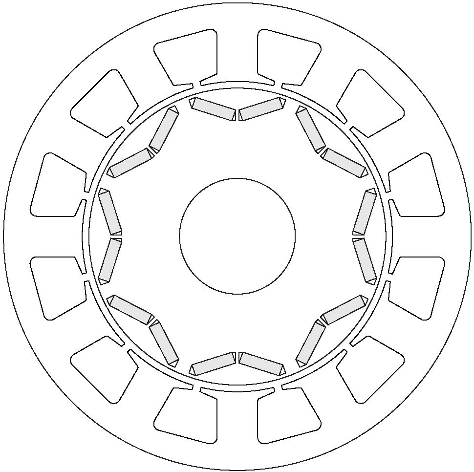
| # poles (p) | 8 | - |
| # stator slots () | 12 | - |
| # turns per slot () | 16 | - |
| Rated current (I) | 97 | A (rms) |
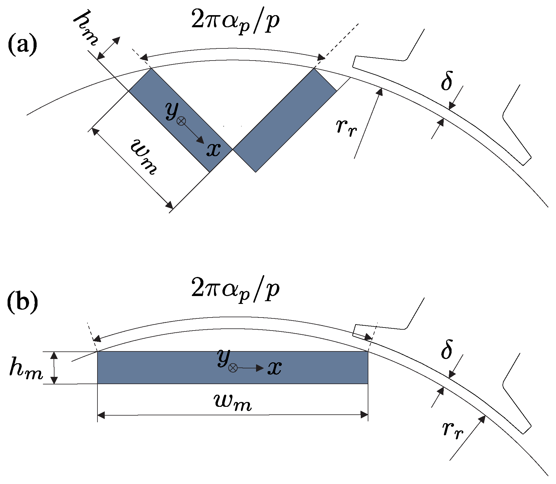
| Rotor radius () | mm | |
| Air-gap length (δ) | mm | |
| Magnet height () | mm | |
| Magnet conductivity () | 694 | kS/m |
| Magnet relative permeability () | - |
References
- Gu, W.W.; Zhu, X.Y.; Li, Q.; Yi, D. Design and optimization of permanent magnet brushless machines for electric vehicle applications. Energies 2015, 8, 13996–14008. [Google Scholar] [CrossRef]
- Lim, S.; Min, S.; Hong, J.-P. Optimal rotor design of IPM motor for improving torque performance considering thermal demagnetization of magnet. IEEE Trans. Magn. 2015, 51, 1–5. [Google Scholar] [CrossRef]
- Ahn, K.; Bayrak, A.E.; Papalambros, P.Y. Electric vehicle design optimization: Integration of a high-fidelity interior-permanent-magnet motor model. IEEE Trans. Veh. Technol. 2015, 9, 3870–3877. [Google Scholar] [CrossRef]
- Kato, T.; Minowa, M.; Hijikata, H.; Akatsu, K.; Lorenz, R.D. Design methodology for variable leakage flux IPM for automobile traction drives. IEEE Trans. Ind. Appl. 2015, 51, 3811–3821. [Google Scholar] [CrossRef]
- Wallscheid, O.; Böcker, J. Global identification of a low-order lumped-parameter thermal network for permanent magnet synchronous motors. IEEE Trans. Energy Convers. 2016, 31, 354–365. [Google Scholar] [CrossRef]
- EL-Refaie, A.M.; Jahns, T.M. Application of bi-state magnetic material to an automotive IPM starter/ alternator machine. IEEE Trans. Energy Convers. 2005, 20, 71–79. [Google Scholar] [CrossRef]
- Yang, Z.; Brown, I.P.; Krishnamurtht, M. Comparative study of interior permanent magnet, induction, and switched reluctance motor drives for EV and HEV applications. IEEE Trans. Transport. Electr. 2015, 1, 245–254. [Google Scholar] [CrossRef]
- Bianchi, N.; Dai Pré, M. Use of the star of slots in designing fractional-slot single-layer synchronous motors. IET Electr. Power Appl. 2006, 153, 459–466. [Google Scholar] [CrossRef]
- Skaar, S.E.; Krøvel, Ø.; Nilssen, R. Distribution, coil-span and winding factors for PM machines with concentrated windings. In Proceedings of the International Conference on Electrical Machines (ICEM), Chania, Greece, 2–5 September 2006; p. 346.
- Bianchi, N.; Bolognani, S.; Dai Pré, M.; Grezzani, G. Design considerations for fractional-slot winding configurations of synchronous machines. IEEE Trans. Ind. Appl. 2006, 42, 997–1006. [Google Scholar] [CrossRef]
- Aslan, B.; Semail, E.; Korecki, J.; Legranger, J. Slot/pole combinations choice for concentrated multiphase machines dedicated to mild-hybrid applications. In Proceedings of the IEEE Industrial Electronics Society (IECON), Melbourne, Australia, 7–10 November 2011; pp. 3698–3703.
- Bianchi, N.; Fornasiero, E. Index of rotor losses in three-phase fractional-slot permanent magnet machines. IET Electr. Power Appl. 2009, 3, 381–388. [Google Scholar] [CrossRef]
- Zheng, P.; Wu, F.; Lei, Y.; Sui, Y.; Yu, B. Investigation of a novel 24-slot/14-pole six-phase fault-tolerant modular permanent-magnet in-wheel motor for electric vehicles. Energies 2013, 6, 4980–5002. [Google Scholar] [CrossRef]
- Bianchi, N.; Bolognani, S.; Fornasiero, E. An overview of rotor losses determination in three-phase fractional-slot PM machines. IEEE Trans. Ind. Appl. 2010, 46, 2338–2345. [Google Scholar] [CrossRef]
- Jahns, T. Comparison of interior PM machines with concentrated and distributed stator windings for traction applications. In Proceedings of the IEEE Vehicle Power and Propulsion Conference (VPPC), Chicago, IL, USA, 6–9 September 2011; pp. 1–8.
- EL-Refaie, A.M.; Bolognani, S.; Fornasiero, E. Fractional-slot concentrated-windings synchronous permanent magnet machines: Opportunities and challenges. IEEE Trans. Ind. Electron. 2010, 57, 107–121. [Google Scholar] [CrossRef]
- Malloy, A.C.; Martinez-Botas, R.F.; Lampérth, M. Measurement of magnet losses in a surface mounted permanent magnet synchronous machine. IEEE Trans. Energy Convers. 2015, 30, 323–330. [Google Scholar] [CrossRef]
- Zhang, P.; Sizov, G.Y.; He, J.; Ionel, D.M.; Demerdash, N.O.A. Calculation of magnet losses in concentrated winding permanent magnet synchronous machines using a computationally efficient finite element method. IEEE Trans. Ind. Appl. 2013, 49, 2524–2532. [Google Scholar] [CrossRef]
- Aslan, B.; Semail, E.; Legranger, J. General analytical model of magnet average eddy-current volume losses for comparison of multiphase PM machines with concentrated winding. IEEE Trans. Energy Convers. 2014, 29, 72–83. [Google Scholar] [CrossRef] [Green Version]
- Böcker, J. 3D analytical model for estimation of eddy-current losses in the magnets of IPM machine considering the reaction field of the induced eddy currents. In Proceedings of the IEEE Energy Conversion Congress and Exposition (ECCE), Montreal, QC, Canada, 20–24 September 2015; pp. 2862–2869.
- Yamazaki, K.; Fukushima, Y. Effect of eddy-current loss reduction by magnet segmentation in synchronous motors with concentrated windings. IEEE Trans. Energy Convers. 2011, 47, 779–788. [Google Scholar] [CrossRef]
- Chalmers, B.J. Electromagnetic Problems of A.C. Machines; Chapman and Hall: London, UK, 1965; pp. 66–87. [Google Scholar]
- Sadarangani, C. Electrical Machines—Design and Analysis of Induction and Permanent Magnet Motors; Universitetesservice: Stockholm, Sweden, 2006; pp. 543–658. [Google Scholar]
- Ruoho, S.; Santa-Nokki, T.; Kolehmainen, J.; Arkkio, A. Modeling magnet length in 2-D finite-element analysis of electric machines. IEEE Trans. Magn. 2009, 45, 3114–3120. [Google Scholar] [CrossRef]
- Krakowski, M. Eddy-current losses in thin circular and rectangular plates. Archiv für Elektrotechnik 1982, 64, 307–311. [Google Scholar] [CrossRef]
- Sinha, G.; Prabhu, S.S. Analytical model for estimation of eddy current and power loss in conducting plate and its application. Phys. Rev. Spec. Top. Accel. Beams 2011, 14, 062401. [Google Scholar] [CrossRef]
- Mukerji, S.K.; George, M.; Ramamurthy, M.B.; Asaduzzaman, K. Eddy currents in solid rectangular cores. Prog. Electromagn. Res. B 2008, 7, 117–131. [Google Scholar] [CrossRef]
- Nategh, S.; Wallmark, O.; Leksell, M.; Zhao, S. Thermal analysis of a PMaSRM using partial FEA and lumped parameter modeling. IEEE Trans. Energy Convers. 2012, 27, 477–488. [Google Scholar] [CrossRef]
- Zhang, H.; Wallmark, O.; Leksell, M.; Norrga, S.; Harnefors, M.N.; Jin, L. Machine design considerations for an MHF/SPB-converter based electric drive. In Proceedings of the IEEE Industrial Electronics Society (IECON), Dallas, TX, USA, 29 October–1 November 2014; pp. 3849–3854.
- Mayer, J.; Dajaku, G.; Gerling, D. Mathematical optimization of the MMF-function and -spectrum in concentrated winding machines. In Proceedings of the International Conference on Electrical Machines and Systems (ICEMS), Beijing, China, 20–23 August 2011.
- Zhao, L.; Li, G. The analysis of multiphase symmetrical motor winding MMF. Electr. Eng. Autom. 2013, 2, 11–18. [Google Scholar]


| \p | 8 | 10 | 12 | 14 |
|---|---|---|---|---|
| 6 | 4.0 | 4.7 | N.F. | 4.1 |
| 9 | N.F. | N.F. | 6.3 | N.F. |
| 12 | 0.8 | 2.0 | N.F. | 6.2 |
| 15 | N.F. | 1.0 | N.F. | N.F. |
| 18 | 0.5 | 0.5 | 1.2 | 4.6 |
| 21 | N.F | N.F. | N.F. | 1.3 |
| 24 | 5.6 | N.F. | 7.7 | |
| 27 | N.F. | 0.8 | N.F. | |
| 30 | N.F. | 0.9 | ||
| N.F. | Not feasible/unbalanced winding | |||
| Distributed windings | ||||
| Low losses | ||||
| Medium losses | ||||
| High losses | ||||
| \p | 8 | 10 | 12 | 14 |
|---|---|---|---|---|
| 6 | 9.8 | 9.8 | N.F. | 6.7 |
| 9 | N.F. | N.F. | 11.3 | N.F. |
| 12 | 1.9 | 4.0 | N.F. | 9.1 |
| 15 | N.F. | 2.0 | N.F. | N.F. |
| 18 | 1.2 | 1.0 | 2.1 | 7.4 |
| 21 | N.F | N.F. | N.F. | 2.2 |
| 24 | 11.5 | N.F. | 12.5 | |
| 27 | N.F. | 1.4 | N.F. | |
| 30 | N.F. | 1.5 | ||
| N.F. | Not feasible/unbalanced winding | |||
| Distributed windings | ||||
| Low losses | ||||
| Medium losses | ||||
| High losses | ||||
© 2017 by the authors. Licensee MDPI, Basel, Switzerland. This article is an open access article distributed under the terms and conditions of the Creative Commons Attribution (CC BY) license ( http://creativecommons.org/licenses/by/4.0/).
Share and Cite
Zhang, H.; Wallmark, O. Limitations and Constraints of Eddy-Current Loss Models for Interior Permanent-Magnet Motors with Fractional-Slot Concentrated Windings. Energies 2017, 10, 379. https://doi.org/10.3390/en10030379
Zhang H, Wallmark O. Limitations and Constraints of Eddy-Current Loss Models for Interior Permanent-Magnet Motors with Fractional-Slot Concentrated Windings. Energies. 2017; 10(3):379. https://doi.org/10.3390/en10030379
Chicago/Turabian StyleZhang, Hui, and Oskar Wallmark. 2017. "Limitations and Constraints of Eddy-Current Loss Models for Interior Permanent-Magnet Motors with Fractional-Slot Concentrated Windings" Energies 10, no. 3: 379. https://doi.org/10.3390/en10030379