A Dynamic Economic Dispatch Model for Uncertain Power Demands in an Interconnected Microgrid

Abstract

In this paper, we propose a dynamic economic dispatch (DED) model with sharing of responsibility for supply–demand balance under uncertain demands in a microgrid (MG). For developing the proposed model, an energy band operation scheme, including a tie-line flow (TLF) contraction between the main grid and the microgrid (MG), is constructed for preventing considerable changes in the TLFs caused by DED optimization. The proposed scheme generalizes the relationship between TLF contractions and MG operational costs. Moreover, a chance-constrained approach is applied to prevent short- and over-supply risks caused by unpredictable demands in the MG. Based on this approach, it is possible to determine the reasonable ramping capability versus operational cost under uncertain power demands in the MG.

1. Introduction

Distributed energy resources (DERs), such as photovoltaics (PVs), wind turbines (WTs), micro turbines (MTs), and storage devices, are expected to play an important role in the electricity supply system and the low-carbon economy in future. However, the greater challenge is to determine the extent to which the DERs may be adopted in a power system. In particular, an excessive supply of DERs will produce a load balancing problem under time-varying power consumption and renewable resource generation [1].

Owing to energy generation limits and economic concerns, the system operator (SO) of a main grid must secure adequate energy resources in advance and solve the dynamic economic dispatch (DED) problem. The DED problem involves determining a method of reducing operational costs based on load demands over the N-step horizon. In computing, it has become increasingly difficult to determine the optimal resource allocation for the DED problem in growing bulk-power systems, and it is impracticable to economically manage individual DERs because of their dimensional and computational complexities. Thus, an interconnected microgrid (MG) can be used to reduce the complexities of the DED problem in a main grid by independently managing the assigned DERs.

To minimize operating costs while considering the forecast of demands in a main grid, several studies have been conducted on the design of control structures and models [2,3]. Accordingly, many DED model designs have been developed for MGs [4,5,6,7,8,9,10,11]. In [4], for example, a centralized controller was proposed to monitor the execution of a scheduling plan, interrupt the monitoring process to input new information, and repair the plan during the execution in each time interval. In a similar study, Chen et al. presented a smart three-phase strategy using forecasting, storage, and management modules [5]. Their study evaluated the economic performance of energy storage systems (ESSs) based on the respective capital, operating, and maintenance costs. To further develop the control algorithms from [4,5], Parisio et al. proposed a linear mixed-integer programming model for DED in an MG without considering the fluctuations in the tie-line flow (TLF) [6], and Olivares et al. proposed an energy management system (EMS), architecture and algorithm for isolated MGs [7]. These studies included unit commitment constraints, selling and purchasing of energy to/from the main grid, and the curtailment schedule. Meanwhile, the distributed or decentralized control structure-based DED models in MG have been also founded. In [8], Mahmoodi et al. proposed a distributed economic dispatch strategy for MGs. Based on this distributed control structure, a centralized optimization problem with computational complexity is decomposed into multiple optimization problems defined over nanogrids. In [9,10,11], the architectures for managing multi-stage operation scheduling are proposed through multi-agent system approach. As a decentralized control structure, these studies were to provide the highest possible autonomy for different DER units and loads. However, in these control structures, the special protocols and procedures to handle the information are yet to be studied [12].

Despite the advances made in the above research, it remains necessary to develop a method of sharing and distributing the power outputs of the controllable generation resources under uncertain demands between the main grid and the MGs. Most of the strategies as per previous studies can increase potential risks or operational costs in the main grid, because those studies focused on computing the control signals by reducing the costs of MG operation even though the main grid is interconnected. This means that TLF, which is not in the isolated MG, is a very important variable to optimize the objective function in the interconnected MG. Besides, more a detailed modeling of the uncertainty should be required to be enough to ensure the reliable operation of the system. This is because determining the amount of energy reserve to be secured is very important for maintaining the system reliability while minimizing operational costs. The primary objectives of our present study are the following.

• Development of a model predictive control (MPC)-based controller for minimizing the MG operating costs, including the cost of load shedding.
• Design of a sharing scheme for demand uncertainties between the main grid and the MG (energy band-based operation scheme).
• Generalization of the relationship between TLF contractions and MG operational costs.
• Contemplation of the change in operational costs according to the reliability level required in the MG.

In order to obtain more an optimal and reasonable solution in the interconnected MG, the centralized control model for DED in MG is designed, and we newly specify the variables required for TLF operation. These variables include the energy contractions in each time interval between the main grid and MG as well as the energy band operation scheme to improve the system reliability. The remainder of this paper is organized as follows. In Section 2, the state transition models for MTs, battery energy storage system, tie-line power flow, and unbalanced demand control are introduced to apply the techniques in the MPC. Section 3 presents the proposed energy band operational scheme to share demand uncertainties between the main grid and the MG. Section 4 presents the design of the chance-constrained approach for considering the demand uncertainties as well as the relationship between system reliability and operational costs in the MG. Section 5 presents the formulation of the objective function through the MPC-based approach. Section 6 illustrates a numerical study conducted on the proposed control model. The conclusions are presented in Section 7.

2. MPC-Based Microgrid System Modeling

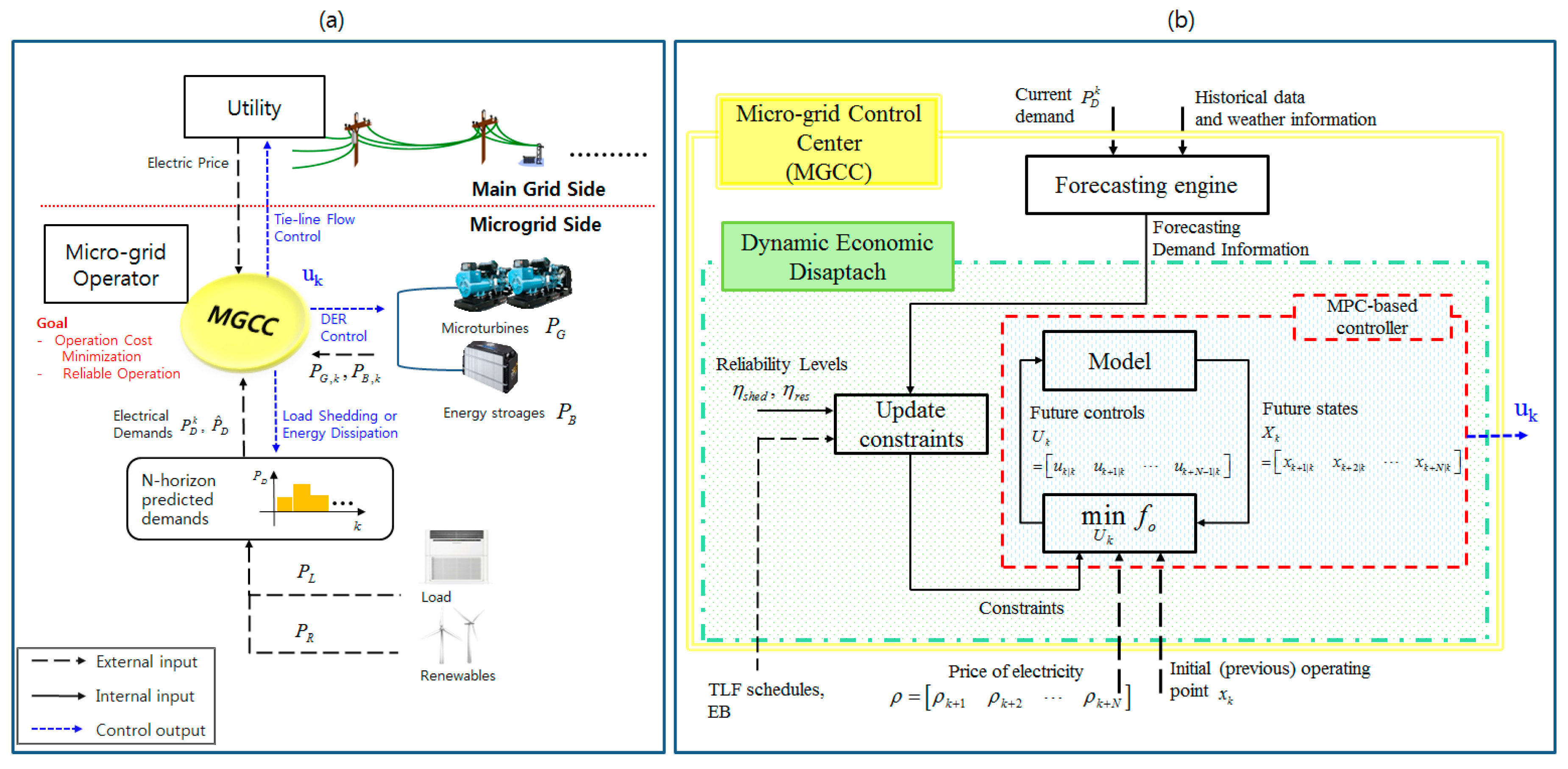
Figure 1 depicts a schematic control diagram for an interconnected MG. As shown in this figure, the present research assumes that the MG is centrally controlled and managed by an MG central controller (MGCC), which has been studied in [13,14], and that the control signals are computed by considering predicted demands over the N-step horizon and energy contracts with the main grid. In this section, the key features of the controllable resources considered in this research are described.

2.1. Micro Turbines

In micro turbines (MTs), the ramp and power output constraints are mainly considered. With these considerations, the state transition model and constraints of N_G micro turbines are defined as:

$$P_G^{k+1}=P_G^k+u_G^k=A_G{P}_G^k+B_G{u}_G^k$$

(1)

$$P_G^k={[\begin{array}{ccccc}{P}_{G,1}^k& \cdots & P_{G,i}^k& \cdots & P_{G,N_G}^k\end{array}]}^T$$

(2)

$$u_G^k={[\begin{array}{ccccc}{u}_{G,1}^k& \cdots & u_{G,i}^k& \cdots & u_{G,N_G}^k\end{array}]}^T$$

(3)

$$P_{G,i}^{\min }\le P_{G,i}^k\le P_{G,i}^{\max },\mathrm{for}1\le i\le N_G$$

(4)

$$u_{G,i}^{\min }\le u_{G,i}^k\le u_{G,i}^{\max },\mathrm{for}1\le i\le N_G$$

(5)

where $A_G$ and $B_G$ are N_G-by-N_G identity matrices.

2.2. Energy Storage

Unlike the case of an MT, the state-of-charge (SOC) and power output constraints are of primary concern in the case of energy storage. This element is not significantly affected by the generation ramp such as in Equation (5); nevertheless, it involves a new and different constraint (e.g., SOC). The state transition and constraints of the battery energy storage can be expressed as:

$$P_{B,i}^{k+1}=B_{dis}{u}_{dis,i}^k+B_{ch}{u}_{ch,i}^k=B_B{u}_{B,i}^k$$

(6)

$$S_{B,i}^{k+1}=S_{B,i}^k+{\eta }_{dis,i}{u}_{dis,i}^k+{\eta }_{ch,i}{u}_{ch,i}^k$$

(7)

$$P_B^k={[\begin{array}{ccccc}{P}_{B,1}^k& \cdots & P_{B,i}^k& \cdots & P_{B,N_B}^k\end{array}]}^T$$

(8)

$$S_B^k={[\begin{array}{ccccc}{S}_{B,1}^k& \cdots & S_{B,i}^k& \cdots & S_{B,N_B}^k\end{array}]}^T$$

(9)

$$u_B^k={[\begin{array}{ccccc}{u}_{B,1}^k& \cdots & u_{B,i}^k& \cdots & u_{B,N_B}^k\end{array}]}^T$$

(10)

$$S_{B,i}^{\min }\le S_{B,i}^k\le S_{B,i}^{\max },\mathrm{for}1\le i\le N_B$$

(11)

$$P_{B,i}^{\min }\le P_{B,i}^k\le P_{B,i}^{\max },\mathrm{for}1\le i\le N_B$$

(12)

$$u_{dis,i}^k\le 0,\mathrm{for}1\le i\le N_B$$

(13)

$$0\le u_{ch,i}^k,\mathrm{for}1\le i\le N_B$$

(14)

In addition, $B_B$ = [1, 1] and $u_B$ = [$u_{dis}$, $u_{ch}$]^T. As shown in Equations (6)–(14), the battery model has two independent control inputs, one for charging, $u_{ch}$, and the other for discharging, $u_{dis}$.

2.3. Tie-Line Power Flows

The state transition and constraints of a single tie-line power flow are given by:

$$P_{tie}^{k+1}=P_{tie}^k+u_{tie}^k=A_t{P}_{tie}^k+B_t{u}_{tie}^k$$

(15)

$$P_{tie}^{\min }\le P_{tie}^k\le P_{tie}^{\max }$$

(16)

where $A_t$ and $B_t$ have a value of 1.

The form of this model is similar to that of the MT state model. However, scheduling $P_{tie}^{k+1}$ in (15) depends on the system marginal prices (SMPs) of the main grid and the MG. In other words, the tie-line power flow is not directly associated with power production and consumption.

2.4. Controls for Unbalanced Power Demands

Two types of uncontrollable resource allocation conditions exist for meeting an uncertain demand: energy shortage and excess supply. In these cases, the control state transition and constraints of the two conditions can be represented as:

$$P_{curt}^{k+1}=u_{curt}^k$$

(17)

$$P_{shed}^{k+1}=u_{shed}^k$$

(18)

$$u_{curt}^k\ge 0$$

(19)

$$u_{shed}^k\le 0$$

(20)

Here, the two control options are energy curtailment in the case of an excess supply, and load shedding in the case of a resource shortage.

2.5. Concatenated State Transition Model

The concatenated state transition matrix in the MG is developed using Equations (1)–(20). The state transition model has the following form.

$$x_{k+1}=A{x}_k+B{u}_k$$

(21)

where,

$$x_k={[\begin{array}{cccccc}{P}_G^k& P_B^k& P_{tie}^k& S_B^k& P_{curt}^k& P_{shed}^k\end{array}]}^T$$

(22)

$$u_k={[\begin{array}{cccccc}{u}_G^k& u_{dis}^k& u_{ch}^k& u_{tie}^k& u_{curt}^k& u_{shed}^k\end{array}]}^T$$

(23)

where both A and B are expressed as a matrix with ($N_G$ + (2 × $N_B$) + $N_{tie}$ + 2)-by-($N_G$ + (2 × $N_B$) + $N_{tie}$ + 2), respectively. Based on Equation (21), the state predictive model over the N-step horizon is given by:

$$\begin{array}{l}{X}_{k|k}=\left[\begin{array}{c}A\\ A^2\\ \begin{array}{c}⋮\end{array}\\ A^N\end{array}\right]x_k+\left[\begin{array}{c}B\\ AB\\ \begin{array}{c}⋮\end{array}\\ A^{N-1}B\end{array}\begin{array}{c}0\\ B\\ \begin{array}{c}⋮\end{array}\\ A^{N-2}B\end{array}\begin{array}{c}\cdots \\ \cdots \\ \begin{array}{c}\ddots \end{array}\\ \cdots \end{array}\begin{array}{c}0\\ 0\\ \begin{array}{c}⋮\end{array}\\ B\end{array}\right]\left[\begin{array}{c}{u}_{k|k}\\ u_{k+1|k}\\ \begin{array}{c}⋮\end{array}\\ u_{k-1+N|k}\end{array}\right]\\ \hspace{1em}=M_x{x}_k+C_u{U}_k\end{array}$$

(24)

3. Energy-Band Operation Scheme

A DED is a long-term operation schedule for minimizing the operating cost of resource generation by forecasting the next N-demands every 5 to 60 min. Operational efficiency and optimization can thus be effectively achieved by sharing the resource and demand information among the participants, including the SO and MG operators.

Compared to the main grid, the MG has the major complication that the demand significantly depends on the uncontrollable power sources [15,16]. Moreover, the demand can have relatively sharp fluctuations caused by a few customers with a large electrical demand. Previous MG studies endeavored to develop an estimation model to forecast the MG demand patterns. Despite the contributions of these models, the demand estimation errors in an MG cannot be ignored owing to the high volatility. 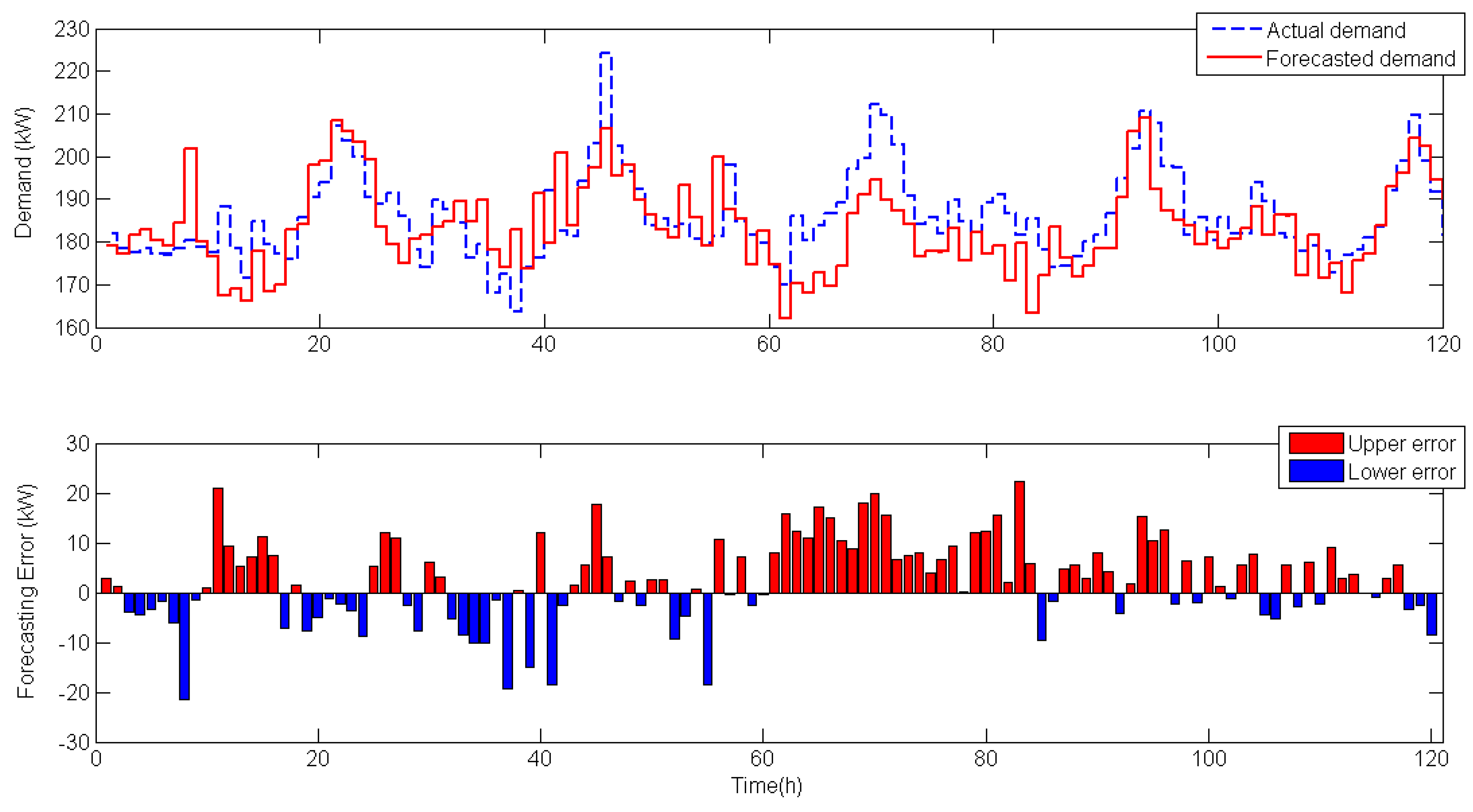Figure 2 shows the differences between the actual power demand and the day-ahead forecasted demand in an MG, with a peak load of approximately 200 kW, in the isolated Gasa Island in Korea [17]. Each demand is calculated as the summation of the load and renewable power outputs. Over the five days of the investigation, this system experienced a large number of forecasting errors owing to the uncertain information on the renewables and loads in the future. Through the existing MG operational scheme, the responsibility for supply–demand balancing is transferred to the SO when this MG system is interconnected with the main grid.

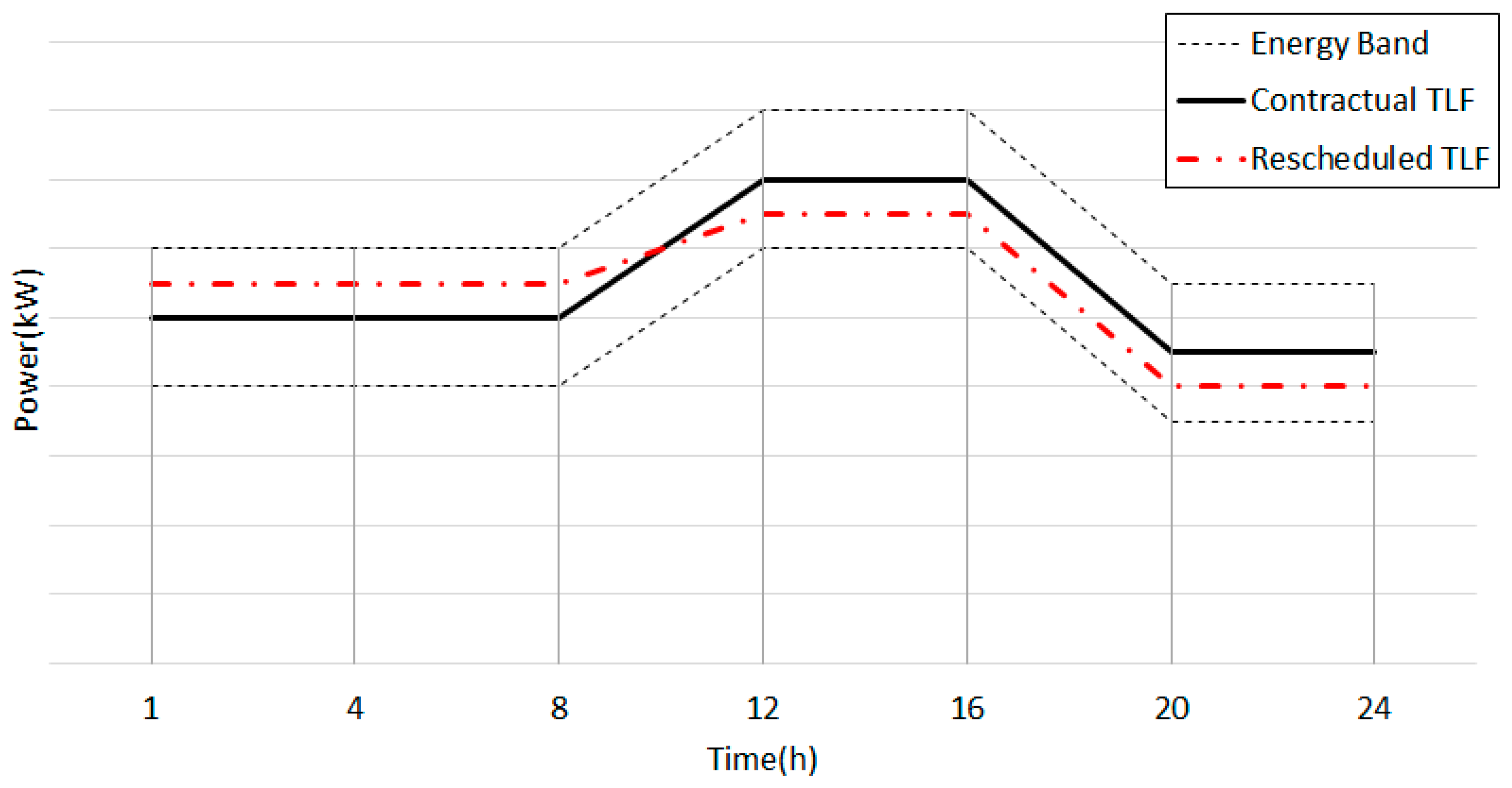
To economically share the uncertainties in an interconnected MG, the present research considers an energy band (EB) operation scheme. Figure 3 shows the basic concept of the EB operation of a TLF. A rescheduled TLF, $P_{tie}^k$, is expressed as:

$$P_{tie,c}^k-P_{tie}^{RB}\le P_{tie}^k\le P_{tie,c}^k+P_{tie}^{RB}$$

(25)

$$P_{tie,c}^{k+1}-P_{tie}^{RB}-P_{tie}^k\le u_{tie}^k\le P_{tie,c}^{k+1}+P_{tie}^{RB}-P_{tie}^k$$

(26)

where $P_{tie,c}$ is the amount of contractual TLF (CTLF), and $P_{tie}^{RB}$ is the size of the energy band used to shift the demand uncertainties to the SO by the CTLF.

Equation (26) describes the new constraints under the multi-stage control and the rescheduled TLF given in Equation (25). In this scheme, there is no additional energy cost for a breach of the CTLF within the EB; this is similar to the previous power exchange market for frequency control [18]. However, in contrast to the exchange market, the rescheduling information should be confirmed with the SO before changing the TLF schedule from $P_{tie,c}$, because it is a schedule of the resource generation and not a short-term operating scheme. This information can assist the SO in minimizing the operating costs and maintaining a stable operation through resource allocation.

4. Designing Chance-Constrained Approach for DED in an MG

Most conventional DED studies have presented precise information: i.e., a known probability mass function with a few events. However, such knowledge is rarely available in practice, and the schedule, computed through a few scenarios, might be infeasible or exhibit poor performance when implemented. This section introduces the proposed chance-constrained approach for the MGCC and contemplates two different standards, the value of lost load (VOLL) and the required system reliability, for optimization.

4.1. Ramping Capability with CTLF Consideration

At each time k, the upward and downward ramping capability (URC and DRC) for the next period, k + 1, is computed as:

$$r_u^k=\left[\begin{array}{l}{\displaystyle \sum _{i=1}^{N_G}\min (P_{G,i}^{\max }-P_{G,i}^k,u_{G,i}^{\max })+\min (P_{tie,c}^{k+1}+P_{tie}^{RB}-P_{tie}^k,P_{tie}^{\max }-P_{tie}^k)}\\ +{\displaystyle \sum _{i=1}^{N_B}\min (\frac{1}{{\eta }_{i,dis}}(-S_{B,i}^{\min }+S_{B,i}^k),-P_{B,i}^{\min }+P_B^k)}\end{array}\right]$$

(27)

$$r_d^k=\left[\begin{array}{l}{\displaystyle \sum _{i=1}^{N_G}\max (P_{G,i}^{\min }-P_{G,i}^k,u_{G,i}^{\min })}+\max (P_{tie,c}^{k+1}-P_{tie}^{RB}-P_{tie}^k,P_{tie}^{\min }-P_{tie}^k)\\ +{\displaystyle \sum _{i=1}^{N_B}\max (\frac{1}{{\eta }_{i,ch}}(-S_{B,i}^{\max }+S_{B,i}^k),-P_{B,i}^{\max }+P_B^k)}\end{array}\right]$$

(28)

where,

$$\max (a,b)=\{y|y\ge a\mathrm{and}y\ge b,y\in \{a,b\left\}\right\}$$

(29)

$$\min (a,b)=\{y|y\le a\mathrm{and}y\le b,y\in \{a,b\left\}\right\}$$

(30)

By securing $r_u^k$, the MG operator can avoid the operational risk caused by resource shortage if the future power demand at time k + 1 is less than the summation of the given power demand $P_D^k$ and the upward ramping capability $r_u^k$. Equation (28) relates to the future energy dissipation (or curtailment) at time k + 1.

In determining the ramping capability, it is necessary to reflect the CTLF and EB, because a change in CTLF affects the demand patterns in the MG; moreover, it may cause load shedding or energy curtailment. For example, the TLF at time k can be set to the maximum value, $P_{tie,c}^k+P_{tie}^{RB}$, while the SMP in the MG is higher than that in the main grid. In this case, the URC from the TLF can have a negative value when $P_{tie,c}^{k+1}$ is lower than $P_{tie,c}^k$. Hence, to reduce load shedding or energy curtailment, the values of URC and DRC should reflect the change in CTLF and EB over the predictive horizons.

4.2. Chance-Constrained Approach for Ramping Capability

To prevent system operation risks arising from resource shortages or excessive supply conditions, the MG operator employs a strategy for determining the proper amount of URC and DRC for future use. In this study, a chance-constrained approach is adopted to maintain an adequate reliability level for the predictive horizon $N_R$, where $N_R\le N$. Assuming that $w_k$ is an independently distributed random variable, which provides the uncertainties of the forecasted demand information, the constraints at each time k have the mathematical form:

$$prob\left({\widehat{P}}_D^{k+1}-{\widehat{P}}_D^k+w_k-r_u^k\le 0\right)\ge {\eta }_{shed}^k$$

(31)

$$prob\left({\widehat{P}}_D^{k+1}-{\widehat{P}}_D^k+w_k-r_d^k\ge 0\right)\ge {\eta }_{curt}^k$$

(32)

Figure 4 shows the method of determining the amount of energy reserve in the proposed approach. In this case, it is assumed that the forecasting engine provides the forecasted demand and the probability distribution function (PDF) of the forecasting errors in each time interval based on the actual demand, weather information, and historical data. Based to this information, the MGCC can handle the supply–demand balance for a designated reliable level, given by Equations (31) and (32). In this case, the chance-constrained approach can be easily realized and implemented, even though most of the chance constraints are nonlinear and difficult to handle, because the cumulative distribution function of $w_k$ in each time interval is a known continuous function. Thus, Equations (31) and (32) can be written in the following form:

$$r_u^k\ge P_u^k$$

(33)

$$r_d^k\le P_d^k$$

(34)

where $P_u^k$ and $P_d^k$ are the minimum and maximum constant values that satisfy (31) and (32), respectively.

Since convex functions guarantee the convexity or concavity of their composition [19], the constraints, given by Equations (33) and (34), are convex. Accordingly, the optimization process can be developed through a numerical analysis method. This research uses sequential quadratic programming (SQR) to optimize the generation resource allocation schedule.

4.3. Value of Lost Load versus System Reliability in Optimization

VOLL, which is the cost of an outage to customers or the price that an average customer would be willing to pay to avoid an involuntary interruption of their electricity supply [20], is an important parameter for managing the MG economically. The MG operator should consider the extent to which the URC is economical according to the VOLL. However, it is a well-known fact that determining the VOLL is very difficult, and the major reasons for the difficulty are as follows.

• Each electricity customer in the power system has different attributes in terms of electricity outage or power quality degradation.
• The value of electricity demand changes with time.
• Load shedding in the power system is an economic problem as well as a reliability problem.

For these reasons, the conventional two-stage or scenario-based approach will have limitations during operation, because they usually assume that the VOLL is a fixed and constant price.

The chance-constrained approach can provide a stable operating condition for the designated reliability level. Therefore, the MG operator can set the reliability level based on extensive consultations with the local customers in the MG. Otherwise, to minimize the operating cost, the MG operator can approach the subject by applying various reliability levels versus a scenario of VOLL over time. In this case, the operational cost can be expressed as a value over the convex curve computed using different degrees of URC.

5. Mathematical DED Formulation

Considering the physical and operational constraints given in Equations (1) to (34), the objective function in (35) represents the cost for the multi-stage operation, including the active power outputs of the controllable DERs, load shedding, and energy dissipation at each time k.

$$\begin{array}{l}\min f_0={\displaystyle \sum _{k=1}^{N}Cos{t}^k}\\ ={\displaystyle \sum _{k=1}^N\left({\displaystyle \sum _{i=1}^{N_G}{C}_i(P_{G,i}^k)}+{\rho }^k{\displaystyle \sum _{i=1}^{N_{tie}}{P}_{tie,i}^k+{\displaystyle \sum _{i=1}^{N_B}{C}_i^{wear}(P_{B,i}^k)-{\rho }^{shed}{P}_{shed}^k}}\right)}\end{array}$$

(35)

where,

$${\displaystyle \sum _{i=1}^{N_G}{P}_{G,i}^k}+{\displaystyle \sum _{i=1}^{N_B}{P}_{B,i}^k+P_{tie}^k}-P_{res}^k-P_{shed}^k={\widehat{P}}_D^k$$

(36)

$$C_i(P_{G,i}^k)=a_i{P_{G,i}^k}^2+b_i{P}_{G,i}^k+c_i$$

(37)

$$C_i^{wear}(P_{B,i}^k)=C_{bw,i}{P}_{B,i}^k$$

(38)

Interestingly, the proposed control scheme computes the optimal signals through a single forecasted scenario. The scenario generation process is required only to develop the PDF at each time rather than to compute the complicated objective functions including multiple scenarios. On the other hand, in the scenario-based approach, which is widely applied in stochastic problems, there is a difficulty in determining the breadth of the scenario of the future [21], because the number of scenarios in the optimization process affects the credibility of the computed solution and also increases the computation cost. Without loss of generality, the computation cost in the scenario-based approach is increased by a factor given by the product of predicted horizon size and the number of scenarios.

During the control process, energy imbalances can occur at the stage k + i because of the high reliability levels required for the demand at the next stage k + i + 1. When a sudden surge of demand arises, the URC is spontaneously decreased, because the operating points of the DERs can be changed near their physical maximum outputs. These outputs may be unable to secure the URC for the next stage. In this case, the strict constraints of the URC can increase the size of load shedding. This means that it is necessary to balance the economic values of the quantity of load shedding at the k + i stage and that it is important to maintain the specified reliability levels for the demand at the next stage (k + i + 1). To manage the MG as flexibly as possible, the option of MGCC reducing the corresponding reliability levels is suggested at the unsettled and unstable time horizons until the levels do not affect the load shedding.

6. Numerical Examples

With the predictive horizon N to 24 h, the proposed EB-based control scheme was implemented by updating the control signals hourly. Analysis was performed on the operation results in the modified Gasa Island MG that involved three MTs and one battery energy storage [17].

Table 1. Simulation data for DERs and tie-line.

Type	Parameters and Values
MT #1	$P_{G,1}^{\min }$	$P_{G,1}^{\max }$	$u_{G,1}^{\min }$	$u_{G,1}^{\max }$	$P_{G,1}^0$
	20	80	−10	10	60
	$a_1$	$b_1$	$c_1$
	0.35	0.095	1.5 × 10−4
MT #1	$P_{G,2}^{\min }$	$P_{G,2}^{\max }$	$u_{G,2}^{\min }$	$u_{G,2}^{\max }$	$P_{G,2}^0$
	20	80	−10	10	50
	$a_2$	$b_2$	$c_2$
	0.40	0.115	1.4 × 10−4
MT #3	$P_{G,3}^{\min }$	$P_{G,3}^{\max }$	$u_{G,3}^{\min }$	$u_{G,3}^{\max }$	$P_{G,3}^0$
	20	100	−10	10	40
	$a_3$	$b_3$	$c_3$
	0.45	0.125	1.2 × 10−4
Tie-line	$P_{tie}^{\min }$	$P_{tie}^{\max }$	$P_{tie}^0$
	−60	60	50
Battery energy storage	$C_B$	$P_B^{\min }$	$P_B^{\max }$	$P_B^0$	ηdis
	80	−10	10	0	1.1/80
	ηch	$S_B^{\min }$	$S_B^{\max }$	$S_B^0$	Cbw
	0.9/80	20	80	50	0

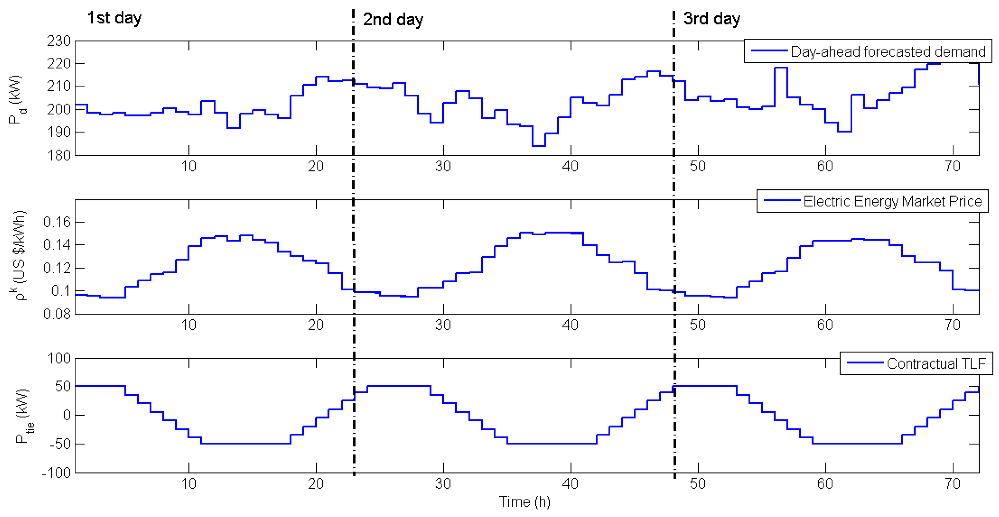
presents the parameters and initial operating points for the given system. To analyze the operational results of the energy storage among different control strategies, the wear cost was assumed as zero. Figure 5 shows the day-ahead forecasted demand, the market prices for electrical energy (or contracted energy prices) at the main grid, and the CTLF schedule for the next 72 h. Here, the CTLF schedule was developed by optimizing Equation (35) based on a deterministic day-ahead forecasted demand. In this simulation, to implement a stochastic environment system easily, it was assumed that $w_k$ in each time interval was represented by an independent and identically distributed random variable with a Gaussian distribution $N({\mu }_k,{\sigma }_k^2)$. In this case, ${\mu }_k$ is designed to ensure that the pattern of the forecasted demand is preserved in the actual demand scenario, and the stochastic demand scenario is generated by an Ornstein–Uhlenbeck mean reverting random walk model as given below [22,23].

$$P_D^{k+1}=P_D^k+\alpha \left({\widehat{P}}_D^k-P_D^k\right)+w_k$$

(39)

$P_D^k$ is the actual demand.

Table 2. Parameters for the stochastic process and value of lost load (VOLL).

Parameter		Value
Mean reverting ratio	$\alpha$	0.7
Mean	${\mu }_k$	${\widehat{P}}_D^{k+1}-{\widehat{P}}_D^k$
Variation	$\sigma$	7.42
VOLL ($/kWh)	${\rho }^{shed}$	3–10

lists the parameters computed by analyzing the data of the Gasa Island MG and the VOLL. This research especially considers various VOLLs in the range of 3–10 $/kWh, because the VOLL significantly affects the operational results, i.e., the operating costs.

6.1. Comparison of MG Operation Strategy

In Figure 6, a comparison of the operation results in the interconnected system are shown for the case when the VOLL is $3/kWh, The MG operator in the given system uses one of the following operation strategies for optimizing the control signals.

(1)

Case 1: As a representative operational strategy of an interconnected MG system, this case does not have the ramping limitation of the TLF, nor does it consider the necessity of securing the URC and DRC.

(2)

Case 2: The MG operator is required to maintain the CTLF within ±20 kW; however, it does not consider the necessity of securing the URC and DRC.

(3)

Case 3: The MG operator maintains the URC over$2\sigma$, which is approximately 97.2%, where $N_R$ = 24. Conversely, the DRC is required to be below −$2\sigma$.

According to the operating conditions of the TLF, the MG operator shares in a different manner the responsibility for the supply–demand balance under uncertain demand changes with the SO. In Case 1, very different TLF results are obtained from the predetermined (contractual) TLF scenario, as shown in region R2 in Figure 6. These results show that the MGCC re-optimizes the control signal schedules for cost minimization with no tie-line ramp (EB) limitations. As an interesting aspect, the TLFs are found to change significantly to about 41.4 kW from 11 h to 12 h with the corresponding change of actual demand of 21.3 kW. Such large changes in region R2 in Case 1 involve an increase in potential risks or operational costs in the main grid, despite a significant reduction in operating costs in the MG The major problem is the decrease in system reliability which is much more critical and important than the operating cost reduction in MG. This means that the scalability, to adopt MGs in main grid, can be limited. In the proposed EB-based scheme, the MGCC optimizes the control signal of the TLF within the EB, as shown in the figure for Cases 2 and 3. Such results are relevant to prevent the extension of operational problems in the MG, i.e., shortages of energy supply to the main grid, even though each operational cost is higher compared to that in Case 1. Therefore, sharing of reliability—i.e., determining the size of the EB as an operating condition—should be carefully considered, because each interconnected system has a trade-off between system reliability and operating cost.

In the proposed EB-based scheme, securing adequate ramping capability in the MG is very important for avoiding the operation risks caused by load shedding or energy curtailment. As shown in Figure 6 for Case 2, the decreased and restricted control for the TLF may accompany the increase for the supply–demand balancing problem in the MG. Specifically, the operational costs in Cases 1, 2, and 3 are $1174.1, $1236.7, and $1184.5, respectively, when the VOLL is $3/kWh. Although the operating cost in the proposed scheme, Case 3, is 0.8% ($10.4) higher than that in Case 1, it is a successful choice compared to Case 2 because the operation cost is reduced about 4.2% ($52.2). These results show that the increased responsibility for the supply–demand balance requires the preparation of a plan for securing the ramping capability of the MG operator.

To pursue profits from energy storage, it is necessary to consider the characteristics of energy storage or the given MG system conditions. Figure 6 shows that the given energy storage, except in Case 3, is not sufficiently recharged to restore SOC; this is to ensure profit by discharging the energy in the future. This is because the round-trip efficiency is set to approximately 82%, which is a normal value of efficiency in the conventional technique [24]. In the given scenario, arbitrage trading—without considering the wear cost—could occur while an SMP in the MG during N predictive demand is at least 1.22 times greater or less with respect to the present condition. This means that the SMPs in the given MG do not have such a difference, even without the wear cost of energy storage. However, the energy storage in Case 3 is better utilized than in other cases, because securing the ramping capability increases the difference among the SMPs in the MG. In particular, the energy storage had a distinguishable charging process from 29 h to 31 h in region R1, which increases SOC about 22.5% even though SOCs over the other cases are reduced or not changed. The reason why the battery was not fully charged is that the charged power was used to secure the URC; the charged power was used for supplying power during the period from 36 to 40 h, which is the time interval with relatively high market price for electrical energy, as shown in Figure 5.

Table 3. Operating costs with different VOLLs.

Parameters		Operation Strategies
		Case 1	Case 2	Case 3
VOLL ($/kWh)	0.2	1174.1	1183.7	1184.5
	0.5	1174.1	1189.4	1184.5
	1	1174.1	1198.9	1184.5
	2	1174.1	1217.8	1184.5
	3	1174.1	1236.7	1184.5

presents the extent to which the operating cost can change with different VOLL settings. It can be seen from Table 3 that the operating costs in Case 2 are largely affected by a change in the VOLL, unlike in Cases 1 and 3. Besides, the amount of load shedding is 18.9 kWh at Case 2. The reason why the operational costs and schedules in Cases 1 and 3 have not changed is the availability of sufficient secured reserves, which completely prevent load shedding. According to the results in Case 3, the reliability level should be carefully determined because the reliability level may be set too high. In other words, the VOLL does not affect the generation schedule developed through the proposed approach once the MG operator decides the reliability level.

Using a computer with an Intel Core i5-3570 CPU @ 3.40 GHz and 8 GB RAM, the average and maximum computation time for optimizing the schedule shown in Figure 6 were recorded as 2.66 s and 4.98 s, respectively. The reason why these impressive results are obtained is that the objective function has a simple convex form. In addition, as mentioned before, the scenario generation process is required only to develop the PDF at each time for determining the URC and DRC based on the designated reliability level. However, in the scenario-based approach, the generated and clustered scenarios should be inserted into the objective function, and this increases the computational complexity.

6.2. Effects of Tie-Line Flow Contraction and Reliability Level

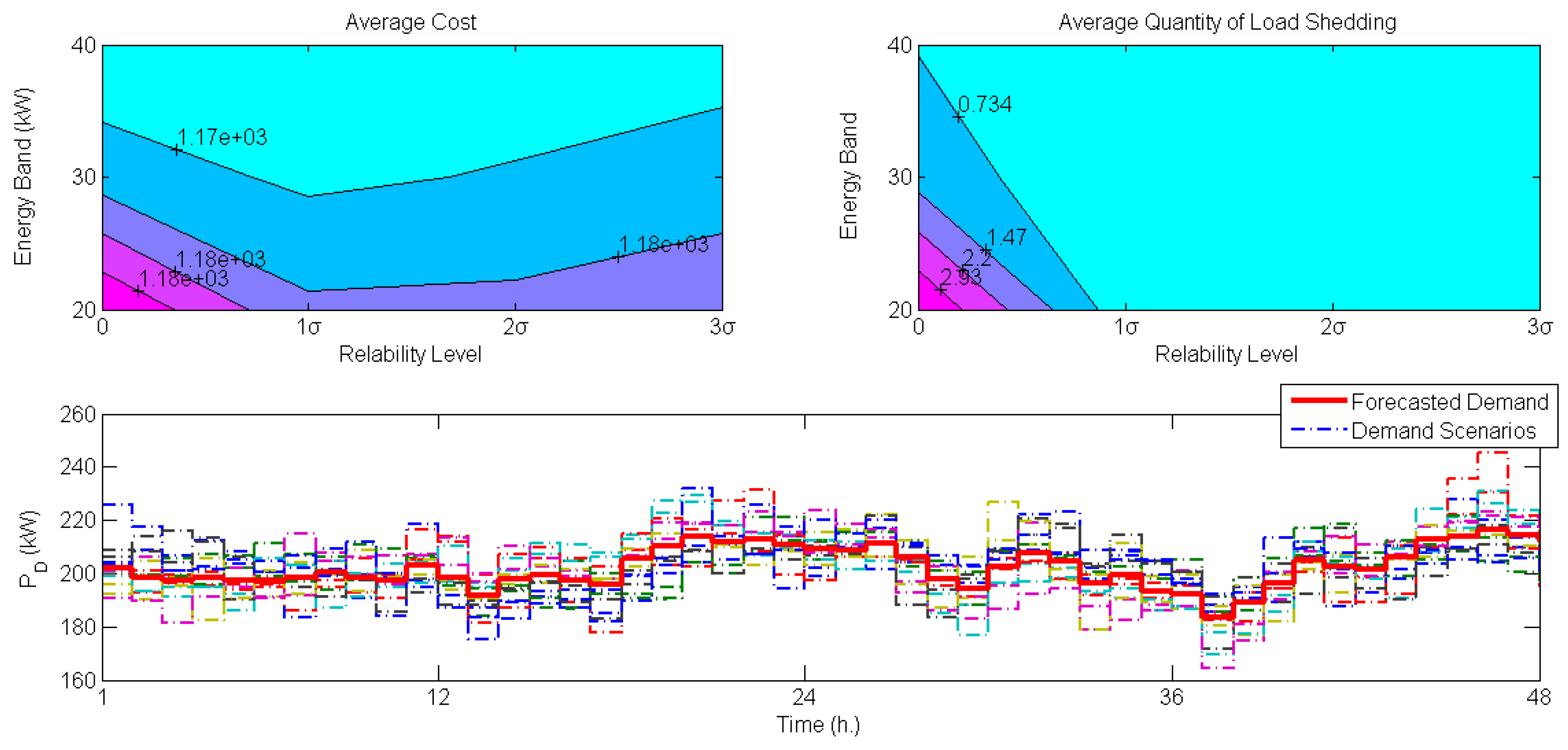
Figure 7 shows the average operation results from 15 randomly generated actual demand scenarios according to different sizes of the EB and different reliability levels. It can be seen that the MG operator can expect a significant decrease in operating cost by expanding the size of the EB. In all cases, when the VOLL is $3/kWh, the operating cost decreases as the EB is further secured. In simulation, the average operation costs (the maximum changes of TLFs) in sizes of EB, 20 kW, 30 kW, and 40 kW, are $1177.6 (38.0 kW), $1773.4 (40.5 kW), and $1170.9 (48.2 kW), respectively, when the reliability level is 1σ. For this, the SO may avoid determining a large size of the EB; however, a small size of the EB can aggravate the economic feasibility in the MG. The current MG systems typically have insufficient economic efficiency on account of high marginal prices or relatively low reliability compared to the main grid. In this case, to lead the MG operators to voluntarily participate in this proposed scheme, additional support—such as incentives for control efforts during uncertain demands, and construction of eco-friendly generation resources—would be required.

It is necessary to secure a proper ramping capability to prevent operation risks and reduce operating costs. As shown in Figure 7, when the MG operator secures a URC of more than $2\sigma$, load shedding almost does not occur, but the operating cost at 1σ is up to 0.7% ($8.4) lower than for the others. This shows that increasing the reliability level decreases the operation risks caused by load shedding; however, securing adequate reserves inevitably incurs additional costs. Based on this relation, the expected average cost is expressed as mentioned before, and a reasonable reliability level is determined by computing the reliability level that responds to the minimum value of the curve.

To minimize the operating cost, the reliability level should be changed according to the operating conditions. In Figure 7, it can be seen that the operating costs at $1\sigma$ are lower than in the other cases. However, $1\sigma$ could not be an optimal choice if the operating conditions are changed. There are two key factors for this. First, expanding the size of the EB is to vitalize energy trading to reduce the SMP caused by uncertain demands in the MG. In simulation for Figure 7, the maximum changes of TLFs in the different sizes of EB, 20 kW, 30 kW, and 40 kW, are 38 kW, 40.5 kW, and 48.2 kW, respectively, when the reliability level is 1σ. From the point of view of the MG operator, the responsibility for balancing supply-demand in MG could be transferred to the SO in main grid, as the use of the expensive generators due to uncertain demand increases could be reduced. Based on these, an MG operator strategy for minimizing the operating costs could be to expand the size of EB more rather than increasing the reliability level. Second, the VOLL is also the key consideration in determining the reliability level. Some sectors of industry, such as mining, place an extremely high VOLL, exceeding 50,000 $/MWh [20]. Clearly, the higher the VOLL that is set in the MG, the higher is the reliability level that is required. This means that the average operating cost curves in Figure 7 should be moved to the right.

7. Conclusions

In this study, an MPC-based controller for optimizing DED problems under uncertain demands in an interconnected MG was developed. The controller optimizes the control signals of MTs, battery energy storage system, tie-line power flow, and unbalanced demand control. In order to reduce operation risks made by the demand uncertainties in MG, the chance-constrained approach was adopted in stochastic process. In simulation, the process was developed by an Ornstein–Uhlenbeck mean reverting random walk model. Based on this approach, this study analyzed the relationship between system reliability and operational costs as well as contemplating the reasonable reliability level in MG. It provided outstanding results in reducing operating costs and preventing energy imbalances within a designated reliability level. In addition, to mitigate the effect of considerable changes in power demands caused by the MG, an EB-based operational scheme was constructed for sharing the demand uncertainties with the main grid. This scheme could prevent potential risks and reduce operational costs in the main grid in comparison with previous studies which focused on only reducing the costs on MG. Based on this scheme, in simulation, the TLF was smoothly managed within the energy band even though the results from existing interconnected MG operational schemes showed that TLF changes sharply. In future research, the authors plan to design the structure of a distributed control model that involves several interconnected MGs.