Optimum Design and Operation of an HVAC Cooling Tower for Energy and Water Conservation

Abstract

The energy consumption increase in the last few years has contributed to developing energy efficiency policies in many countries, the main goal of which is decreasing CO${}_2$ emissions. One of the reasons for this increment has been caused by the use of air conditioning systems due to new comfort standards. In that regard, cooling towers and evaporative condensers are presented as efficient devices that operate with low-level water temperature. Moreover, the energy consumption and the cost of the equipment are lower than other systems like air condensers at the same operation conditions. This work models an air conditioning system in TRNSYS software, the main elements if which are a cooling tower, a water-water chiller and a reference building. The cooling tower model is validated using experimental data in a pilot plant. The main objective is to implement an optimizing control strategy in order to reduce both energy and water consumption. Furthermore a comparison between three typical methods of capacity control is carried out. Additionally, different cooling tower configurations are assessed, involving six drift eliminators and two water distribution systems. Results show the influence of optimizing the control strategy and cooling tower configuration, with a maximum energy savings of 10.8% per story and a reduction of 4.8% in water consumption.

1. Introduction

The increase in energy consumption, as well as CO${}_2$ emissions in the past few decades has become an important and challenging issue. Secure, reliable and affordable energy supplies are fundamental to economic stability and development. In this scenario, governments’ policies tend to be environmentally friendly and energy-saving. As an example, the European Commission 2020 climate and energy package sets three key targets: 20% cut in greenhouse gas emissions (from the 1990 levels), 20% of EU energy from renewables and 20% improvement in energy efficiency. A large proportion of the consumed energy takes place in the residential and services sectors, involving heating, ventilation and air conditioning [1]. The increase in the use of air conditioning systems, which is beginning to be essential due to the new comfort standards, is one of the main reasons for this increase.

Choosing the most suitable configuration and improving the quality and the operation of the devices used in air conditioning systems is one of the available possibilities to tackle this issue. In this regard, cooling towers and evaporative condensers are devices with a high efficiency, which can be used to reject heat in refrigeration cycles, air conditioning or industrial processes. They operate with a low-level water temperature, so that under the same operation conditions, the energy consumption is lower than air condensed devices. Their operation is based on the exchange of mass and energy between sprayed water and an airstream, evaporating a minor part of the water and cooling the rest. The chilled water falls into the tower basin, and the exchanged heat is evacuated by means of the air stream. As a consequence of this operating principle, there is a possibility that some water droplets are captured by the air stream and could escape from the cooling tower. This phenomenon is known as drift, and its associated disadvantages could cause environmental damage and negative effects on human health [2]. Thus, some local governments tend to restrict the installation of cooling towers in some regions despite worsening energy efficiency [3,4]. Furthermore, one of the main challenges in the operation of evaporative condensing systems is to preserve fresh water sources while minimizing energy consumption. The water consumption in the cooling tower includes evaporation and drift, as well as the above-mentioned blowdown. This blowdown water is used to maintain water quality and to avoid scaling and fouling of not only the cooling tower, but also the system heat exchangers. Therefore, the optimization of the cooling tower operation should be two-fold in terms of the components’ design and minimizing energy and water consumption.

In the design of the cooling towers, special attention to three components is provided: the water distribution system and the fill and drift eliminator. Water distribution systems connect the cooling tower with the hydraulic circuit and spread the water over the fill. According to Mohiuddin and Kant [5], this process can be generally carried out by film flow and splash systems, composed by a water canal or nozzles, respectively. Water falls into the cooling tower and is distributed uniformly by the fill, which delays the water fall, and it favors the heat and mass transfer with the air stream. Moreover, to reduce the adverse effects produced by drift, cooling towers have a drift eliminator installed at the exit surface, to minimize the amount of water lost by changing the direction of the airflow.

There are several work in the literature that study the components previously mentioned to assess their influence on the cooling tower thermal performance. Regarding the fill, Thomas and Houston [6] and Lowe and Christie [7] developed heat and mass transfer correlations using cooling towers fitted with different types of fill. Kelly and Swenson [8] studied the heat transfer and pressure drop characteristics of a splash grid type of cooling tower fill. These authors concluded that the properties and geometry of the fill affect the tower characteristic value through correlations with the water to air mass flow ratio. Goshayshi and Missenden [9] experimentally studied the mass transfer and the pressure drop characteristics of smooth and rough surface corrugated fill in atmospheric cooling towers. The results showed that mass transfer performance of the corrugated packing was increased by up to 1.5–2.5-times compared to a smooth packing, and in order to have the maximum mass transfer, the ratio of the pitch to spacing of the corrugation should be of the order of 1.36–1.50. Gao et al. [10] investigated the thermal performance of a wet cooling tower under different layout patterns of fillings, including a uniform layout and four kinds of non-uniform layout patterns. Experimental results manifest that, compared with the uniform layout pattern, the cooling efficiency can be enhanced approximately by 24%–30% under different non-uniform layout patterns.

Besides the fill, drift eliminators and water distribution systems affect the cooling tower’s performance, as well. Hajidavalloo et al. [11] included a brief discussion about the effect of the drift eliminator on the performance of a cross-flow cooling tower taking into account the reduction of the airflow rate. In order to reduce entering dust and suspended solids in the tower, a U-shaped impact separator with a 5% reduction in air flow rate was proposed to place in front of the air louvers of the tower. As a result, no important effect on increasing the outlet water temperature was found, and this may be used easily in front of the towers to filter dusty air. Lucas et al. [12] developed a study to analyze the influence of the drift eliminator on the thermal performance of a draft counter-flow wet cooling tower. The tower characteristic was also correlated with water-to-air mass flow ratios for six different drift eliminators, obtaining an average difference between them of 46.54%. Regarding the distribution system, Lucas et al. [13] analyzed the influence of a film flow (gravity) and a splash (pressure) water distribution system and six different drift eliminators on the cooling tower performance. The obtained results were compared with other works that used a splash-type pressure water distribution system, assessing the best cooling tower performance.

The works mentioned above focus on the thermal performance of cooling towers as an isolated element. However, to find the optimal operating point of a cooling tower incorporated in an HVAC system, it is necessary to study this device in the overall system. Several papers addressing the behavior of a cooling tower linked to an HVAC system can be found in the literature. Jin et al. [14] developed a model of a mechanical cooling tower for the purpose of energy conservation and management. This model was able to predict with simple characteristic parameters the cooling tower performance, validating the results with real operating data from the air conditioning system of a commercial hotel. Engelman et al. [15] compared five different air conditioning strategies for an office building operating in four geographical locations during summer time. They studied the carbon footprints and the grade of comfort. One of the mentioned configurations consists of a cooling tower coupled with a water-water chiller and a fan coil. The results show that this system might be an acceptable solution for buildings in hot summer regions with a high comfort level. However, no control strategies were implemented. Lu et al. [16] developed an optimized model to minimize the energy consumption in the water loop in an HVAC system, analyzing each component and their interactions within and between the cooling tower and chiller. This algorithm was simulated using a centralized pilot plant, with a substantial reduction in operation costs.

The control of the cooling tower fan speed is a key variable in order to reduce the energy consumption of the system. In this regard, some papers report how control strategies affect the overall performance of the system. Chang et al. [17] analyzed a zone temperature method to replace the set-point method of fan control in a cooling tower that uses operational data from an existing variable frequency driver-fan-based system in Taiwan. Savings of 38% for a 0.75 ${}^{\circ }$C zone without increasing the on/off switching frequency were achieved. Some authors have focused their research on optimizing the operation of an air conditions system by setting the power consumption to a minimum. Sayyaadi and Nejatolahi [18] proposed a mathematical study based on three optimization scenarios of a cooling tower assisted with a vapor compression refrigeration system, including thermodynamic and economic single-objective and thermoeconomic multi-objective. The obtained results showed that the multi-objective design more acceptably satisfies the generalized engineering criteria than the other two single-objective optimized designs. Rubio-Castro et al. [19] presented an optimal design algorithm for mechanical draft counter flow wet-cooling towers based on the rigorous Poppe model and mixed-integer nonlinear programming, in order to minimize the total annual cost, which includes capital and operating costs. Results determined that the Poppe method predicts the same optimal values of the tower approach as the Merkel one. However, the Poppe method leads to more reliable optimal designs of wet-cooling towers. Cortinovis et al. [20] developed an integrated model to minimize the operation cost in a cooling water process by optimizing the fan speed, water removal flow rate and valve positions at the heat exchanger branches. It was observed that the outlet temperature of the cooling tower must be kept as high as possible in order to optimize economically the operation of the system. On the other hand, for the cases that require cooler temperatures, the most economical operations are, in this order, increase in the flow rate of the recycle water, increase in the flow rate of the air in the cooling tower and, finally, the forced removal of a portion of the inlet water flow rate to the tower. Sane et al. [21] studied a set of problems in control and optimization in water cooling plants and considered an optimized problem using a dither-based extremum-seeking control to minimize the sum total of chiller and cooling tower power consumption. An improvement of 10% on average was obtained, regarding a commonly-adopted control strategy that maintains condenser water at a constant difference between ambient and wet-bulb temperature. Lu et al. [22] developed a mathematical model of the main components in an HVAC system and implemented an optimization of the energy consumption through a modified genetic algorithm. This optimization problem was transformed and simplified into a compact form to study a pilot-scale centralized HVAC plant, improving the system performance up to 17.2%.

Despite the importance of taking into account both energy and water consumption in a cooling tower at the same time, few works have been reported in the literature on this topic. Marques et al. [23] analyzed an open and closed-loop of a counter flow wet cooling tower to improve the tower’s performance, analyzing its efficiency, considering the water loss through evaporation and the energy consumption in the cooling tower (pump and fans). However, they only include the evaporated water as the amount of water consumed, assuming that drift and blowdown are negligible. Taking into account the price of electric energy in Brazil, an annual energy savings of about US$ 380,000/year was estimated. Chargui et al. [24] worked on a TRNSYS model to take advantage of the water in industrial processes to use it in a cooling tower. The vapor loss is used to run a high capacity heat pump while the rest of the water is connected with a heat exchanger that satisfies the demand of a house in Tunisia. Al-Bassam and Alasseri [25] compared experimentally the effect of installing variable frequency drives instead of dual speed fans in energy and water consumption savings in a cooling tower in Kuwait during the summer season. The results showed a reduction in water consumption of 13% and 5.8% in consumed energy by the fans and chiller for the same amount of cooling produced. For optimization, they incorporated the water consumed as an additional term of energy consumed by using a conversion factor between cubic meters of fresh water and energy needed to produce it in a desalination plant. Although interesting, this approach is only useful in Arabian Peninsula countries. In light of these works, the control optimization and design of cooling towers represent a good strategy for improving energy efficiency and reducing water consumption in HVAC systems.

The main objective of this work is to optimize the design of a cooling tower as a heat dissipation element of an HVAC system and also its operating point, considering the water and energy consumption of the system (cooling tower fan and chiller compressor) in economic terms, while meeting the building cooling demand. To achieve this goal, a model that includes a cooling tower, a water-water cooler and a building was developed. Four methods of capacity control on cooling towers have been considered in the model to carry out a comparative study, taking into account an optimizing control strategy specifically developed to predict and manage the operation point of a cooling tower during simulation and three additional typical control strategies. The secondary objectives are to assess the influence of cooling tower design by analyzing different components (water distribution system and drift eliminator) on the energy and water consumption of the system. For this purpose, the results predicted by transient simulation software, considering twelve cooling tower configurations operating in a Mediterranean location during summer time, have been compared. Furthermore, the model has incorporated the experimental data of thermal performance and drift emissions as part of the previous work of the research group, and also, specific experimental tests have been carried out to fully define the model of the cooling tower in relation to the electricity consumption of the fan.

2. Methodology

The model has been designed by using a transient simulator software, TRNSYS v16 [26], which is able to simulate different systems along a period of time by means of a visual interface based on module connection. This software is recognized as a validating software by the Building Energy Software Tools Directory of the U.S. Department of Energy (DoE) and the International Energy Agency (IEA) [27].

In this work, an air conditioning system comprised of a cooling tower and a water-water chiller has been characterized, in order to meet the demand of a reference building. Four methods of capacity control on cooling towers have also been implemented in order to assess and compare the influence of each of them in the system.

Furthermore, as reported in the previous section, 12 simulations were carried out to determine the influence of the cooling tower elements (drift eliminator and water distribution system) on energy and water consumption of the system in a Mediterranean climate (Alicante, Spain). The cooling tower configurations defined in the work of Lucas et al. [13] were taken as a reference. The authors considered for their experimental tests 6 different drift eliminators (defined from A–F), 2 water distribution systems (pressure water distribution system (PWDS) and gravity water distribution system (GWDS)) and 3 levels for water and air mass flow rates, respectively, for a total of 108 tests. On the one hand, Drift Eliminators A, B and C present a zig-zag structure and consist of fiberglass plates separated at distances of 55, 37 and 30 mm, respectively. Drift Eliminator D is made of plastic as a honeycomb, while Drift Eliminator E is a 45${}^{\circ }$ tilted rhomboid mesh also made of plastic. Drift Eliminator F has the same structure as Eliminator E with a 45${}^{\circ }$ tilted lower half and a 135${}^{\circ }$ tilted upper half. On the other hand, the GWDS consists of a large channel, which covers the effective part of the cooling system outlet section and operates under gravity, while the PWDS is a distribution system equipped with pressure nozzles, which are used to distribute the water droplets uniformly over the packing.

2.1. General Description of the Model

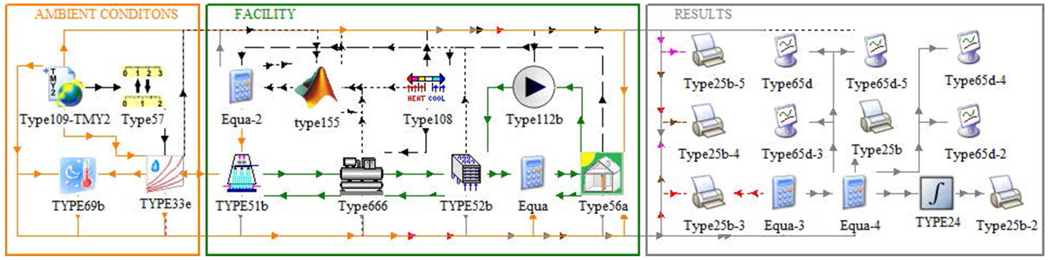
The working modules, usually referred to as types in TRNSYS, involved to represent the installation are depicted in Figure 1. As can be seen, the scheme has been divided into three blocks: ambient conditions, facility and results.

In the ambient block, a typical meteorological year (TMY) as the climate file generated by Meteonorm software [28] is read through type109. This file contains the annual information about meteorological conditions in a geographical location previously set. This information enters as an input in the cooling tower (defined by type51b) and the reference building (type56a) in order to consider its effect on the behavior of these two modules. The facility includes the main components of the model. The cooling tower is connected to the chiller’s condenser (type666) to dissipate the heat that comes from the building through the fan-coil (type52b and type112b). This system is controlled by two additional components. On the one hand, a thermostat (type108) establishes the building set-temperature and controls the start/stop of the air conditioning equipment depending on the building demand. On the other hand, type155 calls external software (MATLAB) to execute a script specifically programmed for this work. It takes the ambient conditions and the information of the current state of the system to calculate the most suitable working point according to each of the four controls implemented. These types are described in more detail later. Finally, the results section saves the simulation data, and it generates charts about the most important variables.

The day with the highest demand has been used to carry out the component selection task. In addition, two considerations have been taken into account: the chiller has to be able to reach to set-point temperature at each simulation time-step, and the demand required by the chiller cannot exceed the nominal capacity of the cooling tower on average while it is working. The air conditioning system satisfies the required energy from the building during the entire year, assuming a time-step of one hour.

2.2. Component Models

2.2.1. Cooling Tower (type51b)

The cooling tower’s performance is modeled via type51b in TRNSYS. This module interacts with the general air conditioning model through one parameter: cooling tower water output temperature. Furthermore, two additional variables provided by this type are used to analyze and compare the control and system performance: power and water consumption.

Cooling Tower Water Output Temperature ($T_{w2}$) Prediction

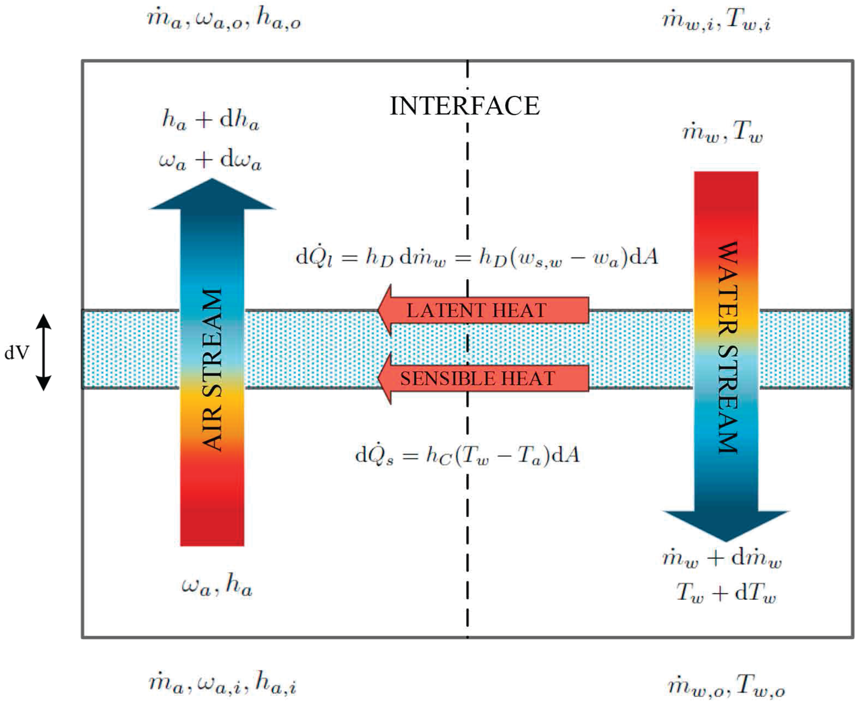
The cooling tower water output temperature ($T_{w2}$) can be calculated through the set of differential equations that predict the evolution of air and water in a counterflow wet cooling tower. These equations can be derived from the governing equations for heat and mass transfer applied to the control volume shown in Figure 2, which represents the schematic of a counterflow cooling tower where the relevant states and dimensions are given. The energy balance at the interface between the water and the air depicts that the heat is transferred from the interface to the air partly as sensible heat (due to the difference in temperature) and partly as latent heat (due to the difference in vapor concentration). The heat transfer due to evaporation is related to the diffusion of water vapor from the water to the interface.

By applying the steady-state mass and energy balances on the incremental volume of Figure 2 simplified by using the following listed major assumptions and the relationships for sensible and latent heat, one can derive, upon rearrangement, the set of differential equations formed by Equations (1)–(3).

• Heat and mass transfer in a direction normal to the flows only.
• Negligible heat and mass transfer through the tower to/from the surroundings.
• Constant water and dry air specific heats.
• Uniform temperature throughout the water stream at any cross-section.
• Uniform cross-sectional area of the tower.

$$\frac{\mathrm{d}{\omega }_a}{\mathrm{d}V}=-\frac{NTU}{V_T}\left({\omega }_a-{\omega }_{s,w}\right)$$

(1)

$$\frac{\mathrm{d}{h}_a}{\mathrm{d}V}=-\frac{LeNTU}{V_T}\left[\left(h_a-h_{s,w}\right)+\left({\omega }_a-{\omega }_{s,w}\right)\left(\frac{1}{Le}-1\right)h_{g,w}\right]$$

(2)

$$\frac{\mathrm{d}{T}_w}{\mathrm{d}V}=\frac{\frac{\mathrm{d}{h}_a}{\mathrm{d}V}-c_{pw}\left(T_w-T_{\mathrm{ref}}\right)\frac{\mathrm{d}{\omega }_a}{\mathrm{d}V}}{\left[\frac{{\dot{m}}_{w1}}{{\dot{m}}_a}-\left({\omega }_{a2}-{\omega }_a\right)\right]c_{pw}}$$

(3)

Here, the Lewis number, Le, represents the ratio of thermal diffusivity to mass diffusivity. It is used to characterize fluid flows where there is simultaneous heat and mass transfer by convection. The number of transfer units (NTU) is the accepted concept of the cooling tower’s performance and measures the degree of difficulty of the mass transfer processes.

$$Le=\frac{h_C}{h_D{C}_{pa}}$$

(4)

$$NTU=\frac{h_D{A}_V{V}_T}{{\dot{m}}_a}$$

(5)

This set of equations may be solved numerically for the exit conditions of both the air and water stream given the inlet conditions and mass flow of both streams and either the outlet air/water temperature or the NTU. The solution is iterative with respect to the outlet air humidity ratio and water temperature (${\omega }_{a2}$ and $T_{w2}$). At each iteration, Equations (1)–(3) are integrated numerically over the entire tower volume from air inlet to outlet.

Effectiveness Model Type51b uses the effectiveness model for cooling towers developed by Braun et al. [29] to predict the cooling tower performance. This model is based on the well-known Merkel [30] model, which relies on two key assumptions: Le = 1 and negligible water loss due to evaporation in the energy balance. According to these simplifications, the equations for the cooling tower may be reduced to:

$$\frac{\mathrm{d}{h}_a}{\mathrm{d}V}=-\frac{NTU}{V_T}\left(h_a-h_{s,w}\right)$$

(6)

$$\frac{\mathrm{d}{T}_w}{\mathrm{d}V}=\frac{{\dot{m}}_a\frac{\mathrm{d}{h}_a}{\mathrm{d}V}}{{\dot{m}}_w{c}_{pw}}$$

(7)

Therefore, by introducing the Merkel assumptions, the solution of Equations (6) and (7) is iterative with respect to a single variable, $T_{w2}$, instead of two variables. However, the solution of Equations (6) and (7) gives only the exit temperature of the water stream and exit enthalpy on the air stream. To obtain the exit humidity ratio, however (necessary to calculate the amount of evaporated water), it is still necessary to numerically integrate Equations (1) after the solution of Equations (6) and (7) has been obtained.

Equation (7) may be rewritten in terms of air enthalpies only by introducing the derivate of the saturated air enthalpy with respect to the enthalpy evaluated at the water temperature.

$$\frac{\mathrm{d}{h}_{s,w}}{\mathrm{d}V}=\frac{{\dot{m}}_a{C}_s\frac{\mathrm{d}{h}_a}{\mathrm{d}V}}{{\dot{m}}_w{c}_{pw}}$$

(8)

where:

$$C_s={\left[\frac{\mathrm{d}{h}_s}{\mathrm{d}T}\right]}_{T=T_w}$$

(9)

$C_s$ is known as saturation specific heat. If the saturation enthalpy were linear with respect to temperature (constant $C_s$), Equations (6) and (9) could be solved analytically for the exit conditions. These equations are analogous to the differential equations that result for a sensible heat exchanger with $C_s$, $h_a$ and $h_{s,w}$ replaced by $C_{pa}$, $T_a$ and $T_w$.

Effectiveness is usually defined as the ratio of the actual to maximum possible heat transfer. However, when $C_s$ is taken as the slope of the straight line between the water inlet and outlet conditions, then the air-side effectiveness rather than an overall effectiveness should be used. The air-side effectiveness is defined as the ratio of the actual heat transfer to the maximum possible air-side heat transfer that would occur if the exiting air stream were saturated at the temperature of the incoming water ($h_{a2}=h_{s,w1}$). The actual heat transfer is then given in terms of this effectiveness as:

$$\dot{Q}={\epsilon }_a{\dot{m}}_a\left(h_{s,w1}-h_{a1}\right)$$

(10)

where, analogous to a dry counterflow heat exchanger, the effectiveness is evaluated as:

$${\epsilon }_a=\frac{1-exp\left(-NTU\left(1-m^{*}\right)\right)}{1-m^{*}exp\left(-NTU\left(1-m^{*}\right)\right)}$$

(11)

where:

$$m^{*}=\frac{{\dot{m}}_a}{{\dot{m}}_{w1}\left(c_{pw}/C_s\right)}$$

(12)

The exit air enthalpy and water temperature are determined from the overall energy balance on the flow streams,

$$h_{a2}=h_{a1}+{\epsilon }_a\left(h_{s,w1}-h_{a1}\right)$$

(13)

$$T_{w2}=T_{\mathrm{ref}}+\frac{{\dot{m}}_{w1}\left(T_{w1}-T_{\mathrm{ref}}\right)c_{pw}-{\dot{m}}_a\left(h_{a1}-h_{a2}\right)}{{\dot{m}}_{w2}{c}_{pw}}$$

(14)

Equation (14) is written in terms of the mass flow rates of water entering and leaving the tower. If the water loss is neglected in the energy balance as in the Merkel [30] method, Equations (10)–(14), along with psychrometric data are sufficient for determining the overall heat transfer conditions. $C_s$ is defined as the average slope of the saturation enthalpy with respect to temperature curve. It is determined with the water inlet and outlet conditions,

$$C_s=\frac{h_{s,w1}-h_{s,w2}}{T_{w1}-T_{w2}}$$

(15)

Since $C_s$ depends on $T_{w2}$, the solution of Equations (10)–(15) is iterative.

In this work, the value for the NTU has been used for closing the set of equations and to determine the tower effectiveness. As suggested by the ASHRAE [31] Equipment Guide, mass transfer data are generally correlated in the form,

$$NTU=\frac{h_D{A}_V{V}_T}{{\dot{m}}_a}=c{\left(\frac{{\dot{m}}_w}{{\dot{m}}_a}\right)}^{1-n}$$

(16)

As general correlations for heat and mass transfer in cooling towers in terms of the physical tower characteristics are not readily available, constants c and n in Equation (16) have been taken from the work of Lucas et al. [13].

Cooling Tower Power Consumption Prediction

The power consumed by the fan of the tower (${\dot{W}}_{\mathrm{fan}}$) is used to compare the performance of the cooling system working under different control strategies and scenarios. The magnitude of the power is expected to depend on the air mass flow rate circulating through the tower (${\dot{m}}_a$). Experimental results for air mass flow rate for the 12 cooling tower configurations taken as a reference in this work can be found in Ruiz [32]. The author found that ${\dot{m}}_a$ not only depends on the fan frequency, but also on the cooling tower configuration and the ${\dot{m}}_w$ level, ${\dot{m}}_a={\dot{m}}_a(f,\mathrm{config},{\dot{m}}_w)$. The influence of the cooling tower configuration is related to the different pressure drop induced into the airstream by the components, whereas the water mass flow influence is explained by the exchange of momentum between air and water streams. Therefore, it is expected that the power consumed by the fans is being affected by the (${\dot{m}}_a$) fan frequency, cooling tower configuration and ${\dot{m}}_w$. 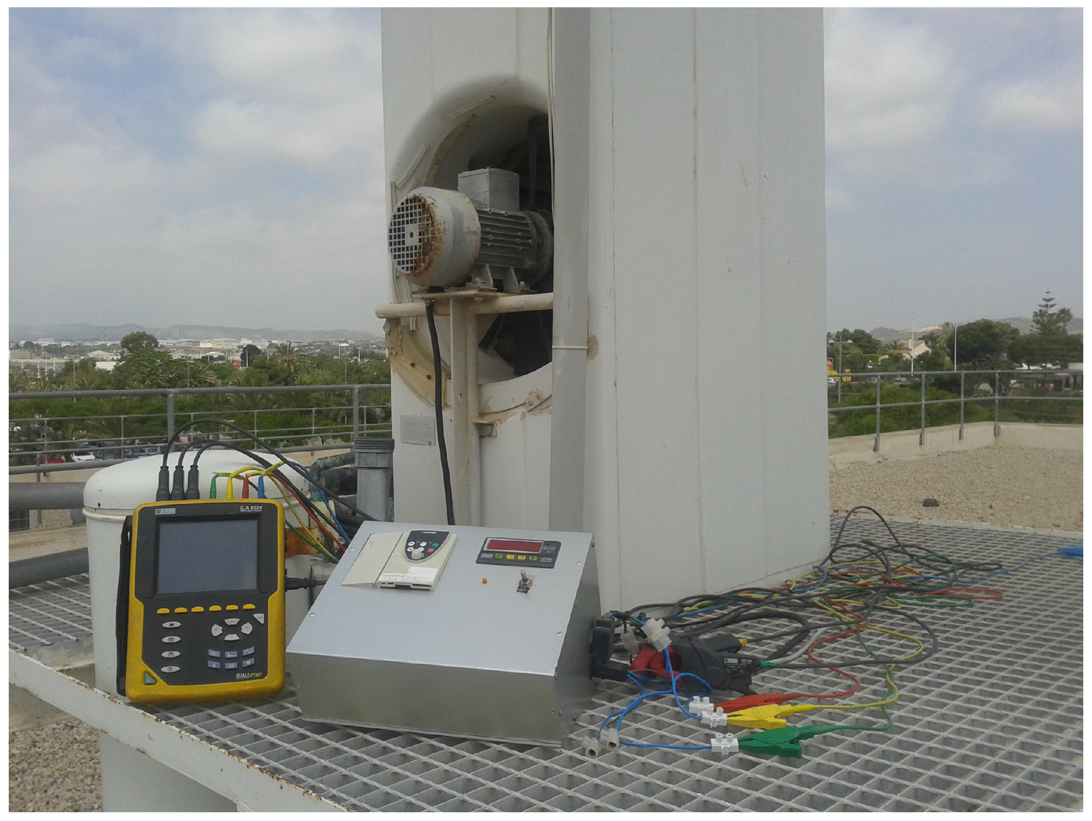As the results for ${\dot{W}}_{\mathrm{fan}}$ for different frequencies and configurations were not initially available in the literature, some ad hoc experiments were conducted in order to assess the validity of the model prediction. In this sense, 120 experimental tests were carried out in the same experimental pilot plant and for all 12 cooling tower configurations (combination of drift eliminator and water distribution system) described in Lucas et al. [13]. The frequency of the fan (f) was fixed at 10 levels (ranging from 5–50 Hz, in 5-Hz intervals). Some additional tests were conducted to analyze the influence of ${\dot{m}}_w$. A Chauvin Arnoux CA 8334 electrical installation tester, with an accuracy of ±0.5% in both tension and intensity, ±1% in power and ±0.01 Hz in frequency, was used in the tests (Figure 3).

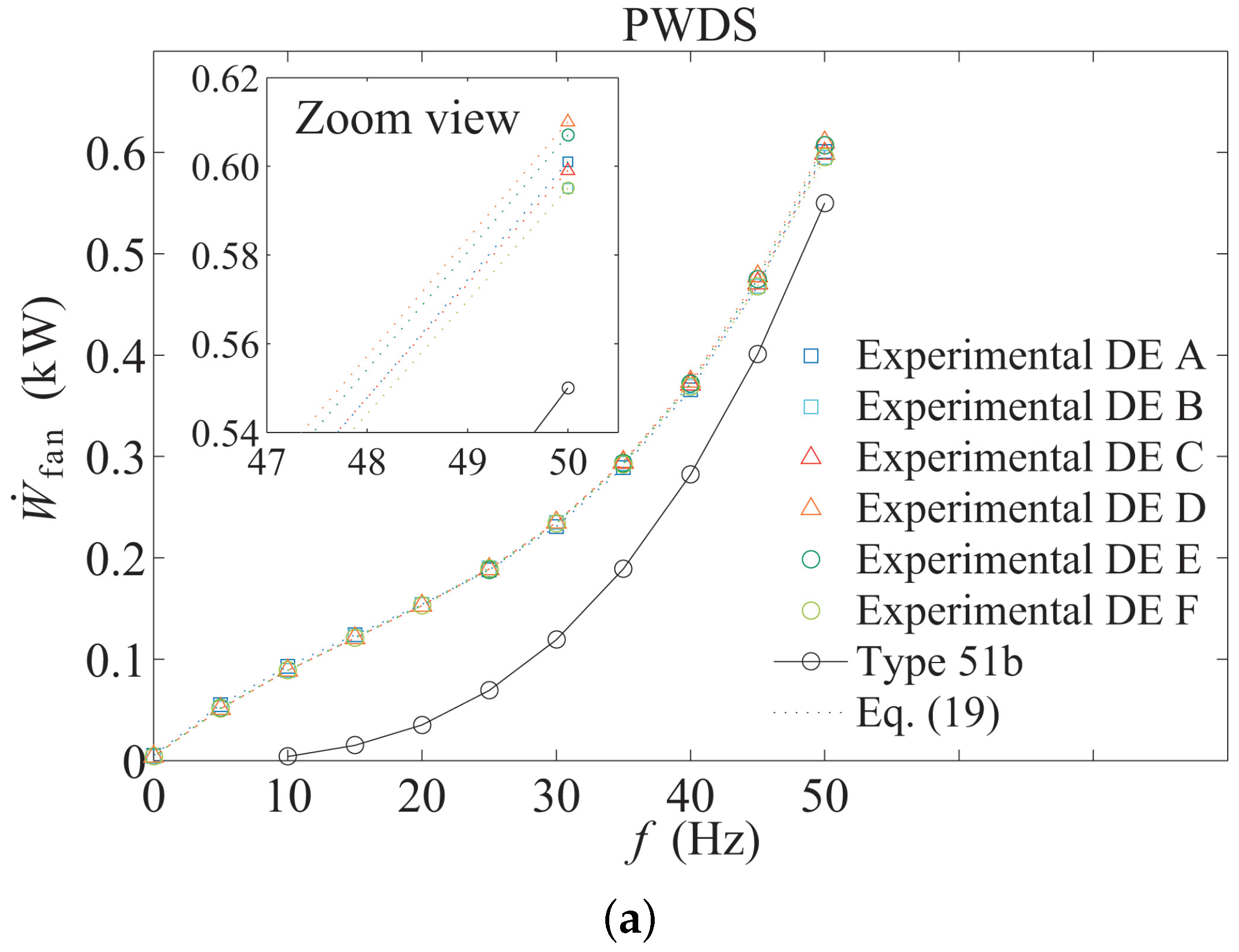
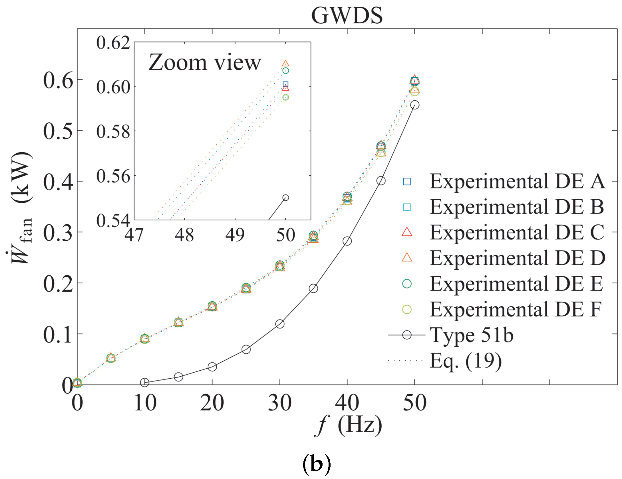
The results for the power consumption experimental tests are displayed in Figure 4. As can be seen, ${\dot{W}}_{\mathrm{fan}}$ is affected mainly by the fan frequency (${\dot{m}}_a$). The influence of the cooling tower configuration was smaller than expected (maximum difference of 5.58% and average of 3.69%) (see left upper figure enlargement), and the ${\dot{m}}_w$ level influence was found negligible (these results are not even shown in Figure 4).

Figure 4 also includes the theoretical behavior of ${\dot{W}}_{\mathrm{fan}}$ defined by type51b (solid line). As can be seen, the pre-defined model differs from the experimental results obtained about power consumption of the tower. This can be justified by the fact that the experimental facility uses a variable frequency drive, which alters the power consumption of the fan adding a factor of efficiency. Moreover, it should be considered that the air mass flow and consequently the power consumption not only depend on the fan frequency as considered by the model, but also on the tower configuration.

Hence, to successfully predict the outlet water temperature and the power consumption of the fan according to the experimental data, it was necessary to obtain the functions ${\dot{W}}_{\mathrm{fan}}={\dot{W}}_{\mathrm{fan}}(f,\mathrm{config})$ and ${\dot{m}}_a={\dot{m}}_a(f,\mathrm{config},{\dot{m}}_w)$. The former is used to compare the performance of the air conditioning system operating in different scenarios, and the latter is used in the thermal performance calculation via the ratio ${\dot{m}}_w/{\dot{m}}_a$. Therefore, an inappropriate modeling of some of these parameters will result in a misleading power and thermal performance prediction.

In this sense, the polynomic equations presented in Equations (17) and (18) were used to link the ${\dot{W}}_{\mathrm{fan}}$ and ${\dot{m}}_a$ with the frequency of the fan, cooling tower configuration and also ${\dot{m}}_w$ in the case of the ${\dot{m}}_a$. The constants for each configuration and equation can be found in

Table 1. Constants for Equation (17).

Configuration	α	β	γ	δ
	[W·Hz${}^{-3}$]	[W·Hz${}^{-2}$]	[W·Hz${}^{-1}$]	[W]
PWDS-A	0.00704	−0.34459	11.54566	4.64615
PWDS-B	0.00626	−0.29466	10.90257	3.66853
PWDS-C	0.00628	−0.29149	10.78880	3.88112
PWDS-D	0.00650	−0.29934	10.82658	3.95944
PWDS-E	0.00661	−0.30910	10.99469	3.50420
PWDS-F	0.00626	−0.29325	10.83723	3.71678
GWDS-A	0.00655	−0.31012	11.01327	3.68462
GWDS-B	0.00688	−0.33929	11.61161	2.05175
GWDS-C	0.00652	−0.30857	11.01921	3.67483
GWDS-D	0.00635	−0.30900	11.08539	3.53916
GWDS-E	0.00635	−0.30136	11.05990	3.26014
GWDS-F	0.00585	−0.27771	10.68402	3.98112

and

Table 2. Constants for Equation (18).

Configuration	${\dot{\mathit{m}}}_{\mathit{a},\mathbf{max}}$	$\mathit{x}\times {10}^9$	$\mathit{y}\times {10}^7$	$\mathit{z}\times {10}^7$	${\mathit{x}}^{\prime }\times {10}^6$	${\mathit{y}}^{\prime }\times {10}^4$	${\mathit{z}}^{\prime }\times {10}^2$	${\mathit{x}}^{\prime \prime }\times {10}^2$	${\mathit{y}}^{\prime \prime }\times {10}^1$	${\mathit{z}}^{\prime \prime }\times {10}^0$
	[kg· h${}^{-1}$]	[h${}^{-2}$·kg${}^{-2}$·Hz${}^{-2}$]	[h${}^{-2}$·kg${}^{-2}$·Hz${}^{-1}$]	[h${}^{-2}$·kg${}^{-2}$]	[h${}^{-1}$·kg${}^{-1}$·Hz${}^{-2}$]	[h${}^{-1}$·kg${}^{-1}$·Hz${}^{-1}$]	[h${}^{-1}$·kg${}^{-1}$]	[Hz${}^{-2}$]	[Hz${}^{-1}$]	[-]
PWDS-A	3148.18	0.09460	−0.05048	0.37426	−0.67950	0.34870	−0.01952	0.09413	−0.24351	0.05077
PWDS-B	3947.54	0.21874	−0.15843	2.65464	−1.81739	1.31301	−0.21864	0.35127	−2.31797	4.11900
PWDS-C	4132.97	−0.20945	0.16038	−2.58101	1.75825	−1.34302	0.21220	−0.34058	2.80877	−4.11206
PWDS-D	3770.53	0.02849	−0.04030	0.99325	−0.19989	0.29741	−0.07719	0.02015	−0.22406	1.24783
PWDS-E	3059.00	−0.11425	0.07863	−1.31778	0.81994	−0.55919	0.09099	−0.13032	1.07447	−1.38599
PWDS-F	3142.05	0.45753	−0.34221	6.03667	−3.68569	2.74174	−0.48699	0.68581	−4.88648	9.09243
GWDS-A	4402.98	0.00217	−0.03071	0.83499	0.32532	0.02083	−0.03215	−0.10400	0.43010	0.10470
GWDS-B	3469.25	−0.08375	0.05941	−1.10113	0.50596	−0.36311	0.07121	−0.04455	0.53083	−0.82314
GWDS-C	4171.26	0.02978	−0.01378	−0.08302	−0.50219	0.30391	−0.02564	0.15544	−0.80898	1.09495
GWDS-D	3741.09	0.34067	−0.22908	3.45193	−2.69013	1.79803	−0.26871	0.49231	−3.08144	4.85449
GWDS-E	2330.40	0.07389	−0.04520	0.41255	−0.63511	0.39548	−0.03896	0.09702	−0.38986	0.52379
GWDS-F	2438.36	0.03954	−0.02633	0.32788	−0.35884	0.24167	−0.03113	0.04567	−0.09154	0.31584

. Values for ${\dot{m}}_{a,max}$ in each configuration have been taken from Ruiz [32]. By implementing Equations (17) and (18) in type51b, it is assured that the model successfully predicts the air mass flow rate power consumption of the fan and thermal performance for a given fan frequency and configuration. This is observed in Figure 4, where the dashed lines represent the results for the model prediction once the set of equations have been implemented in the type.

$${\dot{W}}_{\mathrm{fan}}=3.6\left(\alpha f^3+\beta f^2+\gamma f+\delta \right)$$

(17)

$${\dot{m}}_a={\dot{m}}_{a,\max }\left[{\dot{m}}_w^2\left(x{f}^2+yf+z\right)+{\dot{m}}_w\left(x^{\prime }{f}^2+y^{\prime }f+z^{\prime }\right)+\left(x^{″}{f}^2+y^{″}f+z^{″}\right)\right]$$

(18)

Cooling Tower Water Consumption Prediction

Besides the power consumed by the fans, the other variable used to compare the air conditioning system performing in different scenarios is the water consumption. With regard to cooling tower water consumption, 3 losses have been considered: evaporation, drift and blowdown. Other losses, such as process leaks, have been neglected.

Evaporated water can be calculated from an overall mass balance in the incremental volume of Figure 2. The exit water mass flow rate is,

$${\dot{m}}_{w2}={\dot{m}}_{w1}-{\dot{m}}_a\left({\omega }_{a2}-{\omega }_{a1}\right)$$

(19)

The exit air humidity ratio can be determined by numerically integrating Equation (1) over the tower volume. An alternative approach, which allows an analytic solution, is to assume that Equation (1) is approximately satisfied over the entire tower volume with the local ${\omega }_{s,w}$ replaced with a constant appropriately averaged value. This is known as the effective water surface condition. Assuming Le = 1, integration of Equation (1) gives,

$${\omega }_{s2}={\omega }_{s,w,e}+\left({\omega }_{a1}-{\omega }_{s,w,e}\right)exp\left(-NTU\right)$$

(20)

By integrating Equation (6) for constant $h_{s,w}$, an effective saturation enthalpy can be determined as:

$$h_{s,w,e}=h_{a1}+\frac{h_{a2}-h_{a1}}{1-exp\left(-NTU\right)}$$

(21)

The effective saturation humidity ratio ${\omega }_{s,w,e}$ associated with $h_{s,w,e}$ can be found from psychrometric data. type51b uses this approach (effective water surface condition) to estimate water losses.

Drift losses refer to the amount of total tower water flow escaping the cooling tower. Because of their operation principle, which requires spraying water across or through which a stream of air is passing, water droplets are incorporated into the air stream. Depending on the velocity of the air, it will be taken away from the unit. Drift losses (D) are usually expressed as the ratio between the mass flow of water escaping from the tower (${\dot{m}}_d$) and the total mass flow recirculated by the tower (${\dot{m}}_r$).

$$D=\frac{{\dot{m}}_d}{{\dot{m}}_r}$$

(22)

All of the information needed by TRNSYS to calculate drift losses can be found in the work of Ruiz [32]. The author performed a systematic study (43 tests) by means of the sensitive paper method and determined the D values for all of the cooling tower configurations considered in this paper in several operating conditions.

Finally, blowdown losses (${\dot{m}}_b$) are related to the dissolved solids (such as calcium, magnesium, chloride and silica) remaining in the recirculating water when water evaporates from the tower. As more water evaporates, the concentration of dissolved solids increases, and the solids can cause scale to form within the system. Blowdown consists of removing a portion of the highly concentrated water and replacing it with fresh make-up water. ${\dot{m}}_b$ can be calculated taking into account the cooling tower cycles of concentration ($C_c$). Cycles of concentration represent the accumulation of dissolved minerals in the recirculating cooling water. Analytically, ${\dot{m}}_b$ can be estimated as,

$${\dot{m}}_b=\frac{{\dot{m}}_d+{\dot{m}}_{\mathrm{evap}}}{C_c-1}$$

(23)

In the simulations, $C_c$ was set depending on the hardness of the water ($C_c$ = 1.43 for Alicante, Spain).

Validation of Cooling Tower Model

In order to assess the validity of the cooling tower model, a validation stage was carried out through a comparative analysis between the experimental data available in the literature and the predicted results calculated by TRNSYS. Cooling tower thermal performance was considered to verify the accuracy of the model, assessing the agreement with water outlet temperature and the outlet air mass flow rate.

The results reported in the literature were compared with the predicted results by the model. The ambient conditions recorded during the experimental tests were considered in the simulations. Average differences of 0.7% in outlet water temperature and 2.6% in the air mass flow rate were found between experimental and predicted results.

Figure 5 shows, as an example, the validation of the cooling tower model. In this case, the difference between the results calculated by the model and the experimental ones reported in the bibliography for the cooling tower equipped with Drift Eliminator D and the PWDS can be observed [13]. Here, the differences are below 1% on average for $T_{w2}$ and ${\dot{m}}_a$.

2.2.2. Reference Building (type56a)

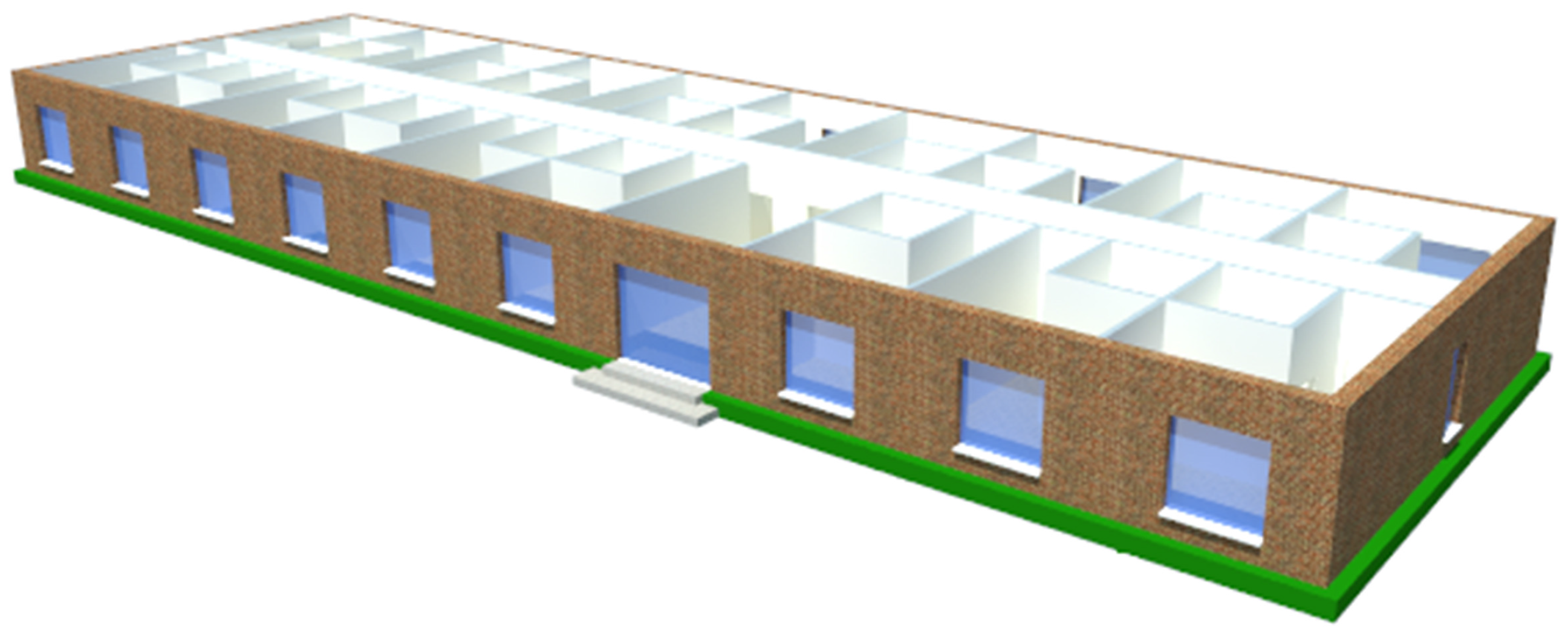
A free-standing one-story hotel building is defined by the module 56a. It is oriented along the east-west axis with an internal access corridor in the center. The glazed area on the north and south facade amounts to 25% of the facade area and 4% on the east and west facade. Figure 6 shows a 3D building model of the hotel. Construction specifications have been taken from the work of Hennin [33], while construction properties meet the requirements set by the European “Energy Performance of Buildings Directive” (EPBD). Nineteen people have been considered simultaneously as a full occupancy during the whole week, there being only two employees at noon. The relevant parameters used in the simulations are displayed in

Table 3. Main hotel properties in TRNSYS.

Building Properties
Area [m${}^2$]	642.6
Wall U${}_{\mathrm{mean}}$ [W·m${}^{-2}$·K${}^{-1}$]	0.24
Wall thickness [m]	0.16
Window u-value [W·m${}^{-2}$·K${}^{-1}$]	1.0
Window g-value	0.58
Solar shading	0.8
Infiltration constant [h${}^{-1}$]	0.5
Volume of air change [m${}^3$·h${}^{-1}$]	900
Room temperature set-point [${}^{\circ }$C]	24

and

Table 4. Internal building loads.

Configuration	Value	Schedule
Laptop [W]	80	9:00–11:00
TV [W]	250	17:00–22:00
Refrigerator [W]	100	00:00–24:00
Lightning [W·m${}^{-2}$]	13	17:00–22:00
Guests [W] [sensible/latent]	[65/55] × 19	00:00–11:00/14:00–24:00
Employees [W] [sensible/latent]	[65/55] × 2	11:00–14:00

.

Regarding solar shading, it works as mechanically-activated shading with external blinds. The solar control is considered as a fraction of the direct radiation on the vertical surface: external blinds are rolled down, reducing the incoming radiation of 80% whenever the solar energy exceeds 200 W·m${}^{-2}$.

There are two different ways to simulate a building with this type: power and temperature level control. On the one hand, the power level control procedure calculates the energy requirements (cooling loads) of the building in each time-step of the simulation, so that it is used for dimensioning and selecting the suitable equipment in order to satisfy the building’s demand. On the other hand, temperature level control allows a realistic behavior, regulating the building’s conditions by means of a thermostat. In refrigeration mode, a cold air stream is used to decrease the temperature of the space taking into account two scenarios. If the equipment is designed properly, the thermostat will turn off the air conditioning system once the setup temperature has been reached. However, if the capacity of the equipment is not enough, the setup temperature will not be met. The first method has been applied to design the air conditioning system, using the second alternative to carry out the simulations. 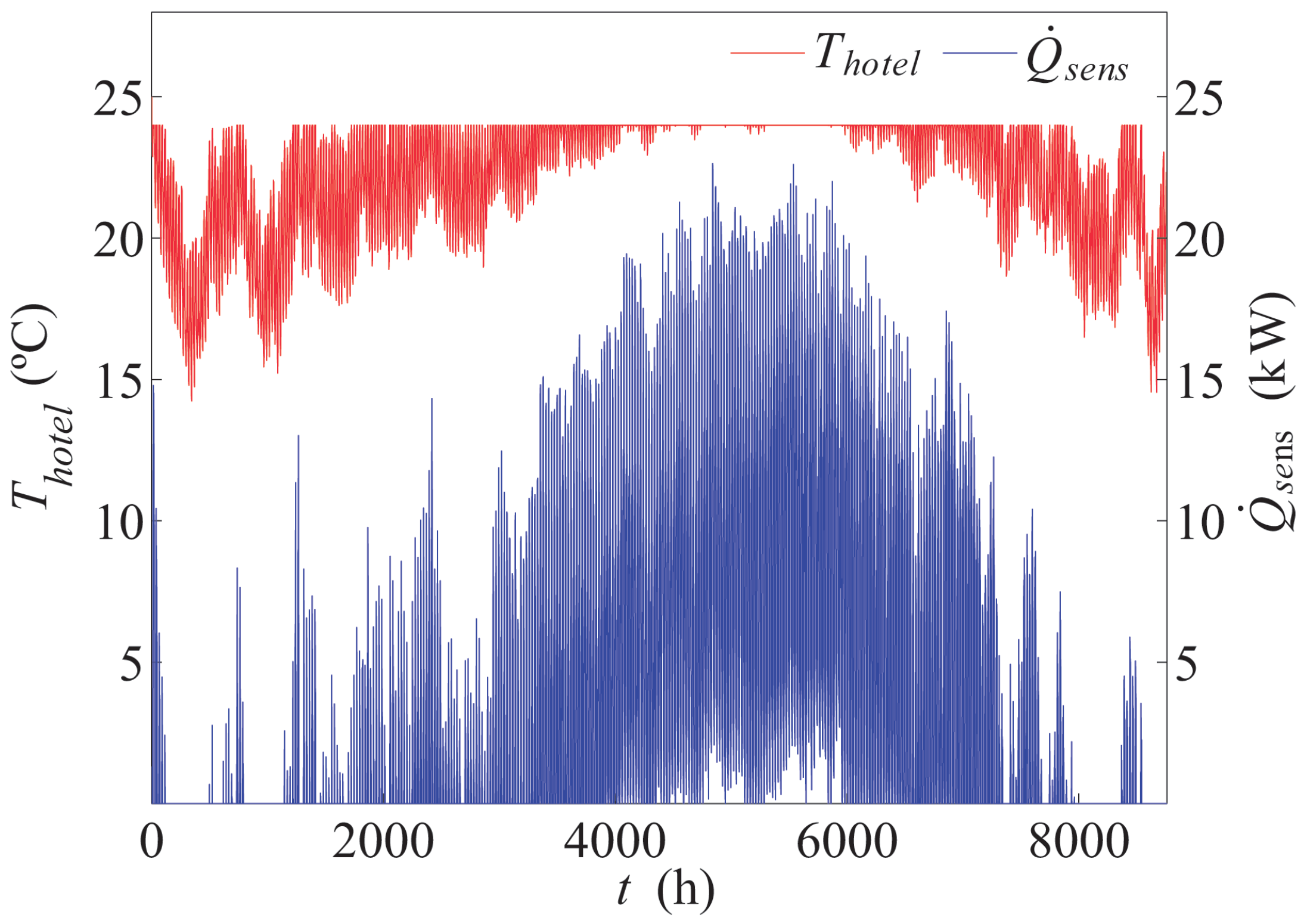Figure 7 depicts the sensible demand of the hotel during a year, using the power level control. Note that the temperature of the hotel does not exceed the design temperature of 24 ${}^{\circ }$C, increasing the demand as necessary until satisfying this condition. Furthermore, it is worth mentioning that the simulation has been carried out for the entire year due to the existence of some occasional moments in which the cooling demand is required during the winter season. Heating mode is not considered in this work.

2.2.3. Chiller (type666)

type666 has been used to model a water/water chiller. This component reads two data files previously defined by the user. The former one provides the capacity and the ratio of the coefficient of performance (COP${}_{\mathrm{ratio}}$) for the values of chilled water set point temperature and entering cooling water temperatures. The latter provides the fraction of full load power for values of the partial load ratio. In that regard, an Airwell brand water-water chiller (Model CWP 09 CO) has been selected to meet the building requirements, with a cooling capacity of 33.7 kW. Nominal COP and capacity at current conditions are calculated as,

$${COP}_{\mathrm{nom}}={COP}_{\mathrm{rated}}{COP}_{\mathrm{ratio}}$$

(24)

$${\dot{Q}}_{\mathrm{ch}}={\dot{Q}}_{\mathrm{ch},\mathrm{rated}}{\dot{Q}}_{\mathrm{ch},\mathrm{ratio}}$$

(25)

The chiller load is calculated by,

$${\dot{Q}}_{\mathrm{load}}={\dot{m}}_{\mathrm{chw}}{c}_{pw}(T_{\mathrm{chw}1}-T_{\mathrm{chw},\mathrm{set}})$$

(26)

The PLR (part load ratio) is therefore,

$$PLR=\frac{{\dot{Q}}_{\mathrm{load}}}{{\dot{Q}}_{\mathrm{ch}}}$$

(27)

If the calculated PLR is greater than unity, type666 automatically limits the load met by the chiller to the capacity of the machine. With a valid PLR calculated (between 0 and 1), the resulting value is the fraction of full load capacity for the current conditions (FFLC). The chiller’s power draw is given by:

$${\dot{W}}_{\mathrm{comp}}=\frac{{\dot{Q}}_{\mathrm{ch}}}{{COP}_{\mathrm{nom}}}FFLC$$

(28)

A corrected COP is then calculated as,

$$COP=\frac{{\dot{Q}}_{\mathrm{met}}}{{\dot{W}}_{\mathrm{comp}}}$$

(29)

The energy rejected to the cooling tower by the device is therefore,

$${\dot{Q}}_{\mathrm{rejected}}={\dot{Q}}_{\mathrm{met}}+{\dot{W}}_{\mathrm{comp}}$$

(30)

and the outlet temperature of the chilled fluid stream is,

$$T_{\mathrm{chw}2}=T_{\mathrm{chw}1}-\frac{{\dot{Q}}_{\mathrm{met}}}{{\dot{m}}_{\mathrm{chw}}{c}_{pw}}$$

(31)

while the outlet temperature of the cooling fluid stream is,

$$T_{\mathrm{cw}2}=T_{\mathrm{cw}1}+\frac{{\dot{Q}}_{\mathrm{rejected}}}{{\dot{m}}_{\mathrm{cw}}{c}_{pw}}$$

(32)

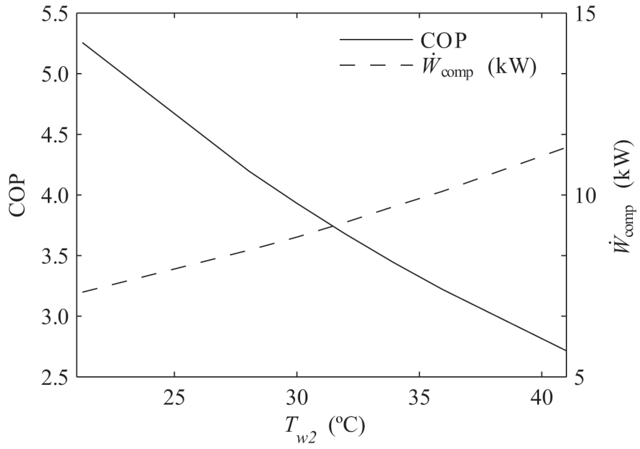
Figure 8 shows the average COP and power consumption as a function of water inlet temperature in the condenser, with a temperature range of 5 ${}^{\circ }$C in the evaporator. As can be seen, the lower $T_{w2}$, the lower power demand required by the chiller’s compressor. The speed of the air in the cooling tower is the key variable to modify the value of $T_{w2}$. A higher fan rotative speed leads to a lower value of $T_{w2}$ and, thus, to a lower chiller power consumption. However, this increase in the rotative speed implies a major power consumption consumed by the fan. Therefore, to improve the performance of the system, it is necessary to reach an optimum fan rotational speed considering it as a tradeoff between all of the variables involved (energy consumption and water losses).

In order to connect the refrigerating system with the building, it was necessary to design a fan-coil, which rejects energy from the ambient hotel with the evaporator’s chiller. This task has been carried out through the types 112b and 52b, using Coolmac Coil Bulletin 5050 [34] to dimension the components through obtaining technical specification, like the number of pipes, rows and fins and, also, the water and air mass flow rate.

The control temperature of the hotel is managed by a thermostat defined with type108. This module controls the starts and stops of the air conditioning system, considering a set-point temperature. A 2 ${}^{\circ }$C hysteresis has also been considered to modify the cooling set temperatures based on the previous state of the controller, in order to avoid continuous starts and stops.

2.2.4. Control Strategies

Four different ways to manage the air conditioning system have been considered in this work through MATLAB software, via type155. This type works as an additional element to the type108 previously mentioned, containing both the cooling tower and chiller model. The capacity control methods implemented are listed below:

• Fan cycling control (FCC).
• Multiple-speed fan motor control in 3 stages of velocity (MSC).
• Frequency-modulating control via VFD (FMC).
• Optimum control (OC).

The FCC is the simplest method of capacity control on cooling towers considered in this work. This control keeps the system working until the thermostat sends a signal once the set-point temperature in the hotel is reached. While the system is working, the fan speed corresponds to f = 50 Hz.

The MSC works by selecting the suitable fan rotational speed that meets the set-point value for $T_{w2}$. Hence, the MSC is an outlet-water temperature-based control. That means that it interacts with the system according to the value of $T_{w2}$. It can work at 3 different frequencies levels: f = 50, 37.5 and 25 Hz.

The FMC involves the use of variable frequency drives (VFD) coupled with a standard fixed-pitch fan. As the MSC, this method is an outlet-water-temperature-based control. The main difference between them is that in the FMC, $T_{w2}$ is kept constant to its set-point by modifying the rotational speed of the fan, whereas in the MSC, just 3 stages can be selected, providing a $T_{w2}$ equal to or lower than the set-point. As a result, this method can provide virtually infinite capacity control and energy management, and it operates efficiently when the tower is at less than full load. A water temperature set-point of 35 ${}^{\circ }$C was considered for MSC and FMC, which corresponds to the regular inlet temperature in nominal conditions for cooling towers.

The fourth and last control, concerning the OC, was developed specifically for this work. The simulations carried out between the cooling tower and water-water chiller have shown a minimum in power consumption at a different point than nominal, regarding the cooling tower fan and chiller compressor. This fact has contributed to finding the optimal operation point in the system, in order to reduce both energy and water consumption in economic terms. To carry out this task, it is necessary to assume the cost of energy and water. In that regard,

Table 5. Energy and water costs.

Measure	Range	Cost	Unit
Energy	-	0.224	€· kWh${}^{-1}$
Water	9 $\ge V_{\mathrm{m}}$	0.962	€·m${}^{-3}$
	32 $\ge V_{\mathrm{m}}>$ 9	1.578
	60 $\ge V_{\mathrm{m}}>$ 32	2.695
	$V_{\mathrm{m}}>$ 60	4.520

shows the usual prices of these two variables in the southeast of Spain (taxes included), considering intervals in the water consumption rates.

3. Results and Discussion

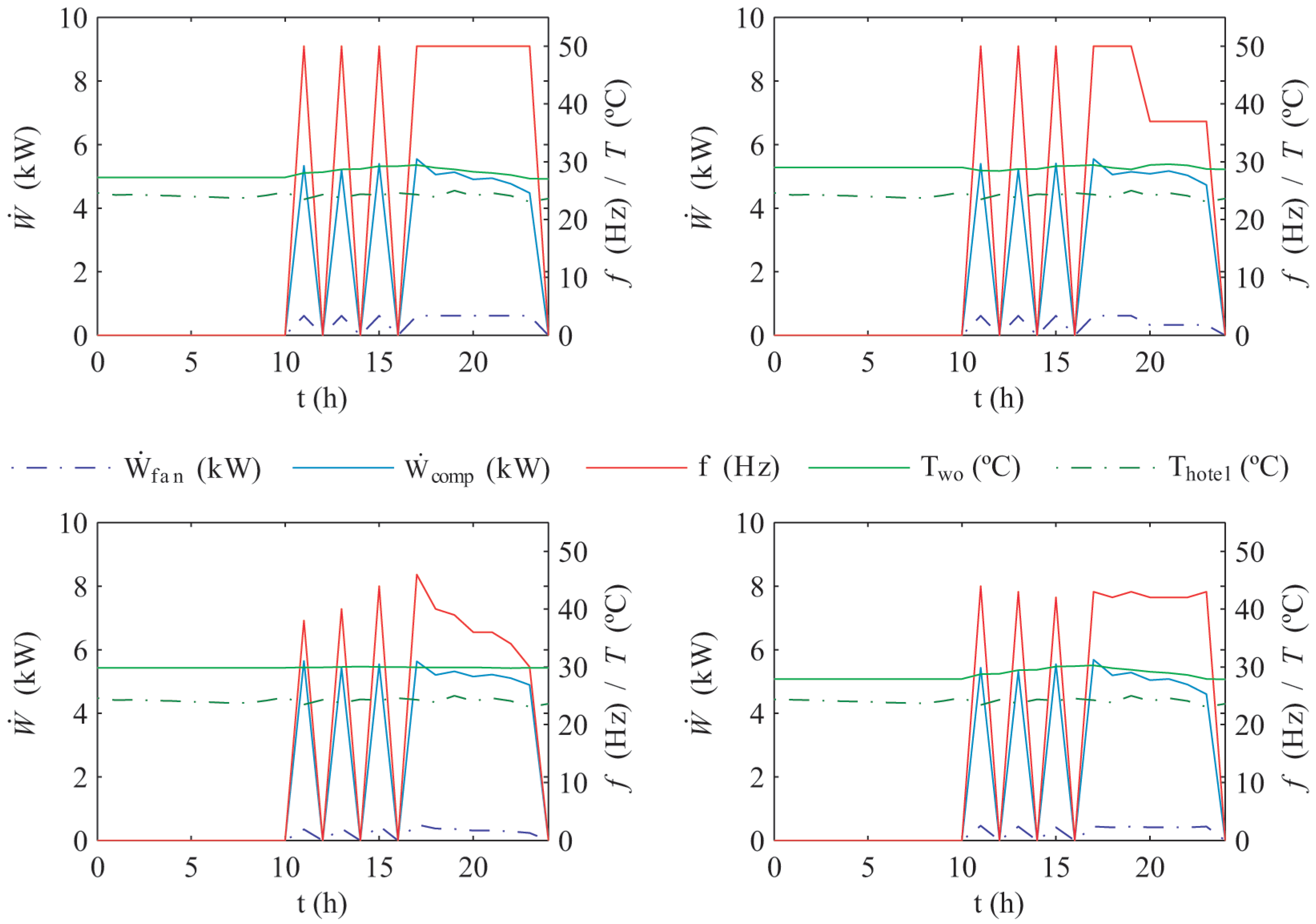
Figure 9 depicts the simulation results of a case study (PWDS and Drift Eliminator D) carried out for each control during a randomly selected day. The charts show the frequency of the fan and the outlet water temperature of the cooling tower, the temperature of the hotel and the power consumption required by the system (fan and compressor).

As can be seen, the FCC control operates at the constant frequency of 50 Hz when there is cooling demand, and it stops working whenever the hotel temperature is below the set-point. The $T_{w2}$ control methods, FMC and MSC, show similar behavior, with the caveat that the former one uses a wide range of frequencies that allows the system to get the water temperature set-point more accurately than the MSC, which uses only three stages of frequency. In the OC, the air conditioning system works in a different set-point than nominal during the simulations. By setting the optimizing control strategy and assuming a cost of energy and water consumption, the overall cost is minimized while meeting the referenced building’s thermal loads. This fact assesses the conclusions of Braun and Diderrich [35], who reported the benefits between a system operating with an optimizing control strategy and another working at nominal conditions, regarding the interaction of the cooling tower with the water-water chiller. The OC control calculates the optimum frequency to get a minimum total cost (water and energy) while the system meets the building load. In all cases, the hotel temperature varies in a range around the set-point temperature. This is due to the hysteresis of the thermostat and the temperature level control mentioned in the last section. The area under the power consumption curves of the fan and the chiller represents the energy demanded by the system, and it will be used for comparative purposes.

A summary of the results predicted by TRNSYS simulations during a whole year for the 12 test runs is shown in

Table 6. Simulation results.

Test	Config	${\dot{\mathit{W}}}_{\mathbf{fan},\mathbf{FCC}}$	${\dot{\mathit{W}}}_{\mathbf{comp},\mathbf{FCC}}$	V${}_{\mathbf{tot},\mathbf{FCC}}$	${\dot{\mathit{W}}}_{\mathbf{fan},\mathbf{MSC}}$	${\dot{\mathit{W}}}_{\mathbf{comp},\mathbf{MSC}}$	V${}_{\mathbf{tot},\mathbf{MSC}}$	${\dot{\mathit{W}}}_{\mathbf{fan},\mathbf{FMC}}$	${\dot{\mathit{W}}}_{\mathbf{comp},\mathbf{FMC}}$	V${}_{\mathbf{tot},\mathbf{FMC}}$	${\dot{\mathit{W}}}_{\mathbf{fan},\mathbf{OC}}$	${\dot{\mathit{W}}}_{\mathbf{comp},\mathbf{OC}}$	V${}_{\mathbf{tot},\mathbf{OC}}$
Run		[kWh]	[kWh]	[m${}^3$]	[kWh]	[kWh]	[m${}^3$]	[kWh]	[kWh]	[m${}^3$]	[kWh]	[kWh]	[m${}^3$]
1	PWDS-A	914.31	7868.83	179.03	734.43	8115.69	179.02	610.70	8324.59	178.57	780.72	7984.65	178.90
2	PWDS-B	905.90	7925.09	172.60	714.88	8170.18	173.04	607.93	8336.06	172.92	730.77	8061.45	172.65
3	PWDS-C	913.21	7908.48	171.43	729.32	8144.71	171.44	613.20	8334.73	171.17	750.70	8032.97	170.94
4	PWDS-D	928.00	7992.24	171.08	731.76	8217.39	171.36	630.60	8355.53	171.13	689.93	8169.51	171.09
5	PWDS-E	923.10	8019.19	170.69	758.59	8201.77	170.85	652.43	8378.02	170.86	724.55	8174.35	170.74
6	PWDS-F	906.54	8117.43	170.66	766.80	8293.39	170.95	680.87	8421.47	170.79	777.32	8230.28	170.69
7	GWDS-A	909.60	8094.18	171.12	844.19	8217.73	171.36	740.35	8410.87	171.14	902.81	8106.35	171.32
8	GWDS-B	906.32	8311.25	171.07	794.99	8427.69	171.20	723.71	8533.06	171.24	740.26	8438.89	171.13
9	GWDS-C	911.72	8310.46	171.10	794.25	8423.79	171.26	722.28	8530.97	171.18	703.29	8457.54	171.24
10	GWDS-D	881.64	8285.69	170.99	804.23	8396.14	171.20	727.15	8514.00	171.04	860.61	8306.49	171.12
11	GWDS-E	907.91	8796.20	171.80	868.15	8843.78	172.28	822.36	8888.53	172.21	737.77	8924.19	172.45
12	GWDS-F	876.79	8602.50	171.29	812.34	8672.32	171.71	758.69	8736.19	171.65	701.31	8731.29	171.82

. Each row contains the results concerning the cooling tower configuration, regarding energy consumption (fan, compressor and total) and water loss (evaporation, drift, purge and total).

3.1. Influence of the Optimizing Control Strategy

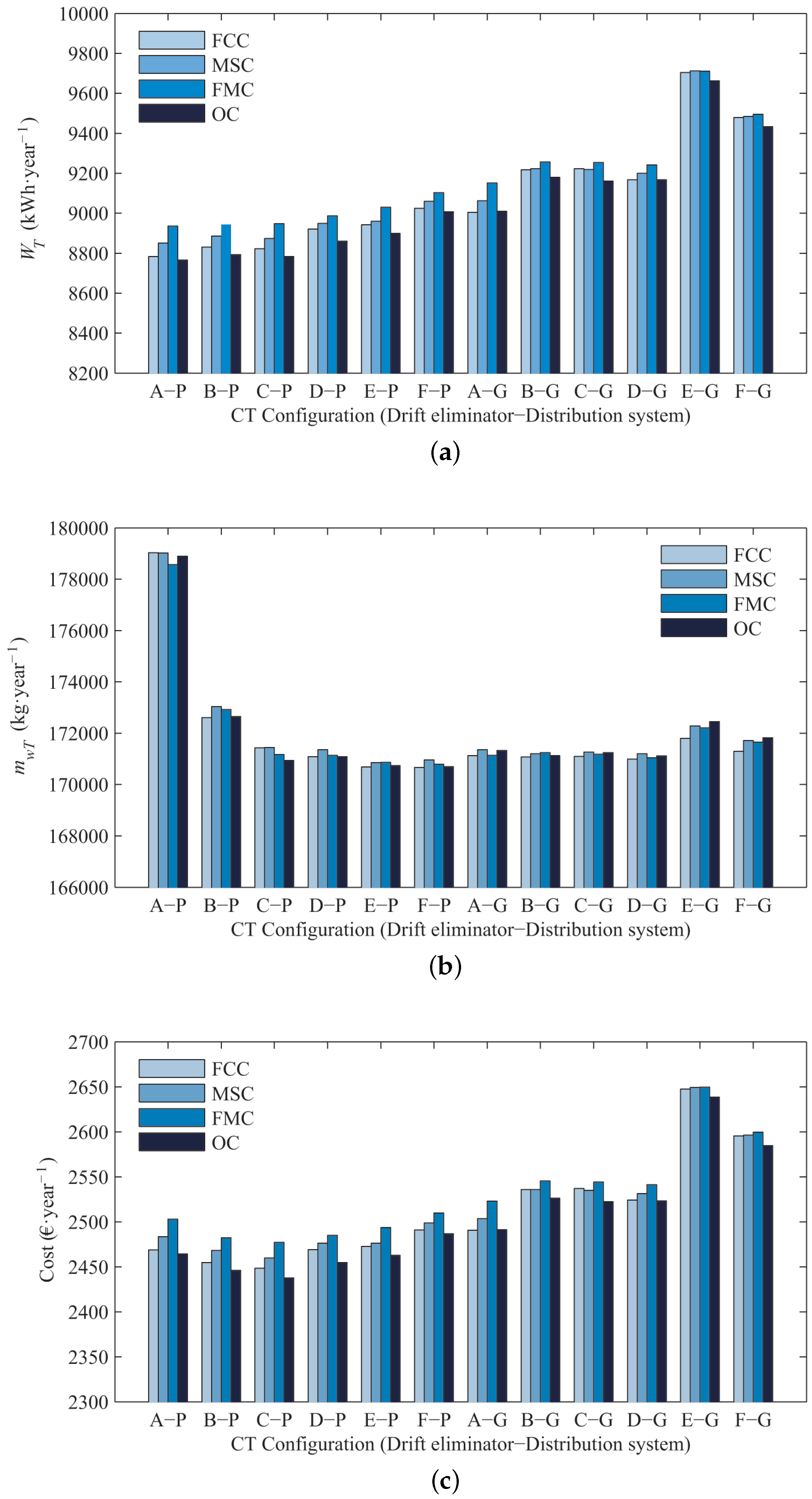
Regarding the influence of the optimizing control strategy, Figure 10 shows the energy, water consumptions and the operation cost obtained for all of the cooling tower configurations and system controls implemented.

Regarding energy consumption, the general trend observed is that the OC operates with a lower energy consumption, followed by FCC, FMC and MSC. The reason that explains why OC requires less energy than the others controls is related to the higher cost of energy compared to the cost of the water. Therefore, although the total cost is optimized in this control, the cost of the energy has a higher relative weight than the cost of the water. The $T_{w2}$-based controls provide the worst results related to energy consumption in all of the simulations performed. This is related to the relative contributions to the total energy consumption of the fan and compressor chiller. 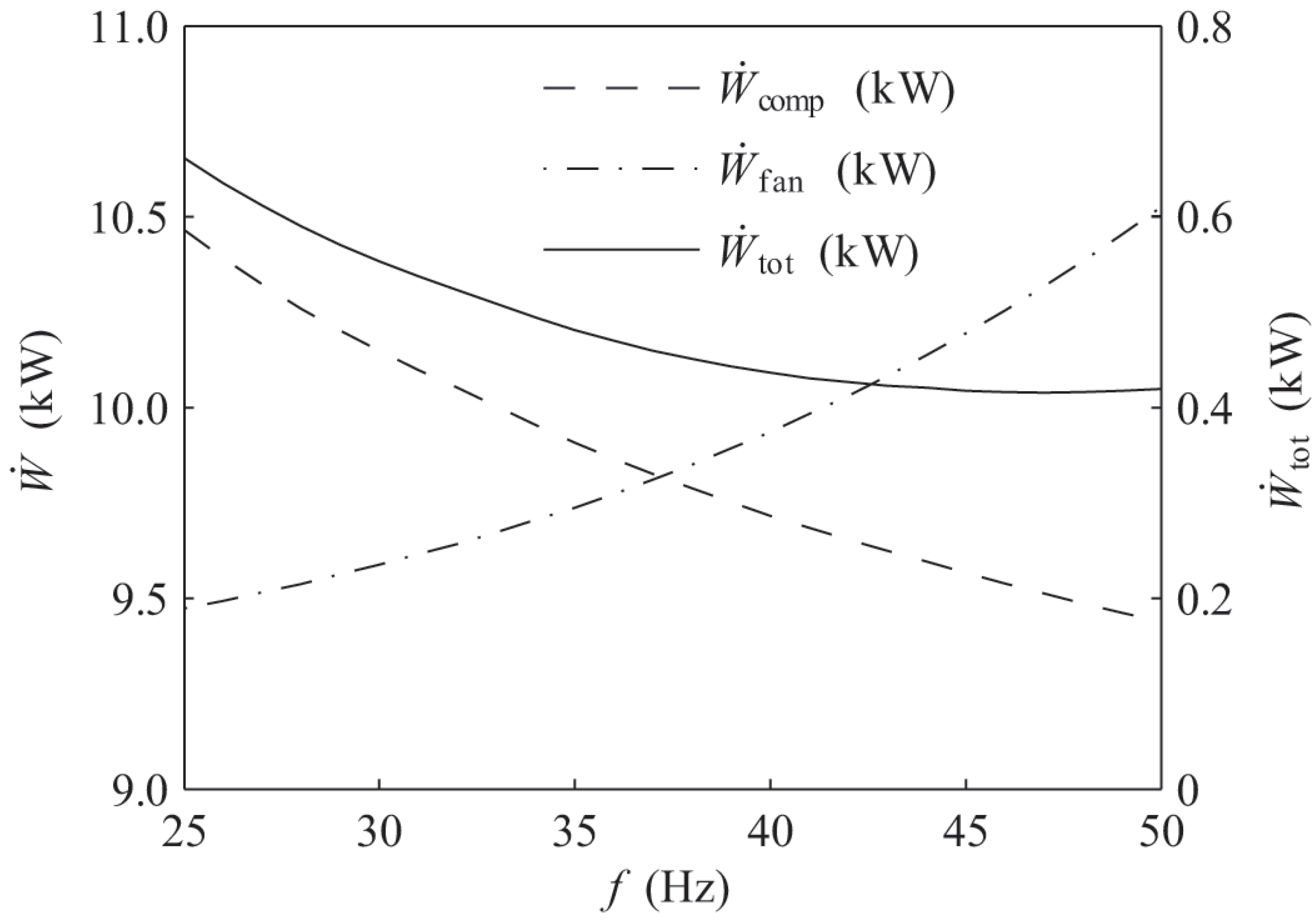Figure 11 depicts the relationship between the power of the chiller compressor and the cooling tower fan with the rotational speed of the fan. As can be seen, the averaged variation per hertz in the compressor consumption is 60% greater than the fan. For that reason, it is necessary to reduce the temperature of the water as much as possible taking into account the power consumption of the fan. As has been mentioned before in this section, the set-point for $T_{w2}$ was set to 35 ${}^{\circ }$C, established by the typical operation point of the cooling towers recommended by the manufacturer. As the outlet water temperature of the cooling tower depends on the ambient conditions and frequency, by setting a control based on a constant temperature, the cooling capacity of the cooling tower can be decreased by reducing the fan velocity in order to get the set-point temperature. This increment in the water outlet temperature of the cooling tower results in a higher power consumption by the compressor of the chiller (without considering the interaction between the fan and compressor), and that is the reason why FMC and MSC controls require more energy to operate the system. Simulations carried out considering different $T_{w2}$ set-points supported this conclusions. When the $T_{w2}$ set-point was set to the lowest attainable temperature allowed by the chiller ($T_{w2}$ = 21 ${}^{\circ }$C), the expected results were obtained: the more intelligent the control is, the more efficiently the system operates (lower energy and costs). The results of these simulations reported the expected sequence of capacity control methods considering the energy consumed by the system ${\dot{W}}_{\mathrm{tot},\mathrm{FCC}}\ge {\dot{W}}_{\mathrm{tot},\mathrm{MSC}}\ge {\dot{W}}_{\mathrm{tot},\mathrm{FMC}}\ge {\dot{W}}_{\mathrm{tot},\mathrm{OC}}$. As the $T_{w2}$ set-point decreases, the energy absorbed by the system decreases, as well. In the limit, if the $T_{w2}$ set-point is set to a certain value that the system cannot reach, it will always work at 50 Hz, and hence, it will behave as the fan cycling method. The explanation given for the fact that the power consumption using MSC is lower than FMC is related to the lower outlet water temperatures provided by the MSC. While the FMC maintains the set-point temperature of the system hertz by hertz, the MSC does not have this capacity of modulation, and a set-point temperature or lower is calculated with the three frequency stages.

Taking into account a comparison between different controls using the same cooling tower configuration, the average difference in power consumption between the OC developed and the others that were considered is 0.77%, with a maximum observed variation of 1.94% using the FMC, in particular with Drift Eliminator A and PWDS. As mentioned before, a different frequency than nominal can result in an optimal operation point, but an inappropriate temperature can result in a major operation cost in the system.

Regarding water consumption, no substantial differences have been found between controls. In general terms, FCC is the control that requires less water, followed by FMC, OC and MSC. This phenomenon could be explained due to evaporation processes. With a lower frequency, the temperature of the water of the cooling tower rises, resulting in a greater evaporation that also affects the purge process. It can be mentioned that the configuration with PWDS and Drift Eliminator A has a water consumption considerably higher than the others due the drift rates reported in the experimental data.

A maximum variation of 0.30% between controls (OC and MSC) is observed for the combination Eliminator C and PWDS. The fact that the variations are so small is due to the major part of the water loss coming from the purge process (70%) and evaporation (29.7%), with the drift influence being very low (0.3%).

Concerning the costs, the OC is the least expensive way to manage the air conditioning system, followed by FCC, MSC and FMC, as a way of weighing the energy and water consumption and their costs. The observations reported in the energy comparison are valid here because the energy expenses are greater than the water expenses. Using one control or another can lead to a maximum savings of 1.62% using the FMC and Drift Eliminator C and PWDS. Depending on the configuration of the cooling tower, the savings in costs can vary by up to 39.51 € per story (1.17 €·kW${}_{\mathrm{installed}}$${}^{-1}$). The design of the air conditioning system has been performed taking into account an appropriate optimization of the equipments, that is why the savings obtained is lower than what can be achieved in an oversized system. This is not a common situation, keeping in mind that the majority of the systems are oversized [21].

3.2. Components Influence

The second part of the results is focused on the influence of the cooling tower configuration in the air conditioning system. The optimizing control strategy is used to calculate these results. The comparatives are depicted in Figure 12, taking into account the energy consumption, water loss and the cost of both variables.

The comparison of the water distribution systems shows that energy consumption using pressure is lower than using the gravity system, with an average difference of 4.7% and the highest variation registered of 8.6% with Drift Eliminator E. This fact is due to the pressure system spraying water in small particles, increasing the exchange surface with the air stream and enhancing the refrigerating process, so that the system requires a lower energy consumption. The opposite situation takes place regarding water loss, in which the pressure system shows greater water consumption than gravity. This fact could be explained considering the physical properties of the water droplets previously mentioned. In this sense, a greater water evaporation is provided by the pressure system. Moreover, it is more likely that these small droplets are rejected from the cooling tower through the drift eliminator. Results show that the calculated average quantity of water lost by drift is 16.4 times greater than gravity. The average savings of total water loss is 1.2%, and the maximum is 4.4% using Drift Eliminator A. In economic aspects, the result of changing the water distribution systems is an average savings of 1.0%, corresponding to 25 €/year per story (0.74 €·kW${}_{\mathrm{installed}}$${}^{-1}$). The maximum saving is 2.1% (Drift Eliminator F), which means 54 € saved per year per story (1.60 €·kW${}_{\mathrm{installed}}$${}^{-1}$). As previously mentioned, this fact is due to the small water particles produced by the pressure system, which obtains a better heat exchange with the same air flow rate, decreasing the energy consumption, but increasing the water loss.

Regarding the drift eliminator influence, using the PWDS can produce a maximum savings of 2.8% between Drift Eliminator F and A and can achieve 7.2% with the difference between Drift Eliminator E and A with GWDS. Results about the water consumption show that changing the drift eliminator with PWDS, it is possible to save a 4.8% from A to F, compared with the 0.8% between E and D of GWDS. As the previous case, the opposite results are obtained with water loss. A great water loss reduction can be achieved changing the drift eliminator in a pressure system, but it is more recommendable to use a gravity system. The drift eliminator influence, as equal to the water distribution system, is due to this component’s affecting the thermal behavior of the cooling tower, because they act as an additional exchange surface of mass and energy. On the one hand, considering PWDS, the average saving about changing the drift eliminator with a PWDS is about 1%, which means 21 €/year per plant (0.62 €·kW${}_{\mathrm{installed}}$${}^{-1}$), with a maximum variation between Drift Eliminator F and C of 49 € (1.46 €·kW${}_{\mathrm{installed}}$${}^{-1}$) (2.0%). On the other hand, the average savings in GWDS is 57 € per year per story (2.7%) and a maximum savings of 147 € (4.37 €·kW${}_{\mathrm{installed}}$${}^{-1}$) (5.9%) changing the drift eliminator from E to A. As mentioned in the above scenarios, although a major savings is obtained with PWDS regarding water loss, it is better to use GWDS. As can be seen, it is necessary to pay attention not only to energy consumption, but also to water loss. Taking into account only one of these two parameters is not enough to make a decision. The best solution in energy consumption could be the worst in water loss. In that regard, the economic variable is considered to link both aspects.

4. Conclusions

In this study, the influence of a capacity control method on a cooling tower operating within an air conditioning system in order to reduce the energy and water consumption in economic terms was developed and assessed. Four control methods were implemented in an HVAC system comprised by a cooling tower, as a heat dissipation device and a water-water chiller connected to a reference building in order to meet the cooling demands. Once the improvement of the proposed control has been tested and compared to those usually used in practice, special attention was paid to the influence of the cooling tower components: the water distribution system and drift eliminator. The main conclusions obtained in this study where a total of 48 simulations was carried out (four control methods and 12 cooling tower configurations) may be summarized as follows:

• A new method to control HVAC systems was developed. Compared to the traditional control methods used in practice (fan cycling, multiple-speed fan motors or frequency-modulating controls), significant savings in the overall operation costs can be achieved (up to 0.7% depending on the cooling tower configuration). The usual $T_{w2}$-based controls provided the worst results related to energy consumption and cost in all of the scenarios considered in the simulations (even worse than the simplest FCC method). This fact has been assessed by the influence of the water temperature on the compressor consumption. An appropriate operation criterion should take into account the relative influence of the fan frequency on the cooling tower output water temperature alongside the power absorbed by the fans. A higher temperature can result in a major cost in the system because of the compressor consumption of the chiller.
• The cooling tower configuration has a direct influence on the energy and water consumption of the air conditioning system. Both the water distribution device and drift eliminator affect the thermal behavior of the cooling tower, working as an additional surface of mass and energy exchange. Changing the combination of these two elements can result in an improvement of 10.2% in energy savings between Drift Eliminator E and GWDS and Drift Eliminator A with PWDS. The water consumption can be reduced to 4.8%, from Drift Eliminator A and PWDS to Drift Eliminator F and PWDS. In economic terms, costs can be reduced to 8.2%, from the configuration with GWDS and Drift Eliminator E to PWDS with Drift Eliminator C.
• Taking into account the maximum saving achievable considering the four control systems presented and the twelve configurations of the cooling tower, it is possible to achieve a savings of 212.25 € per story (6.30 €·kW${}_{\mathrm{installed}}$${}^{-1}$) between the optimization system with Drift Eliminator C and PWDS and the water temperature control with VFD (FMC) using Drift Eliminator E and GWDS.
• Considering an average hotel with 300 rooms in the southeast region of Spain, energy costs can be reduced to 3240 € per year by using the proposed capacity control method. This scenario corresponds to the operation with minimum costs. This value can increase to 36% in oversized systems, according to the research carried out in this study (9.28 €·kW${}_{\mathrm{installed}}$${}^{-1}$, 312.87 € per story, 4382 € per year in the reference hotel).
• The results presented in this paper could eventually assist engineers to select the suitable equipment and system control of an HVAC system. The selection of the components and the control method described above was based on economic parameters. However, the results provided in this work may also be used to define additional criteria based on specific situations.