1. Introduction
Nowadays, the increasingly prominent environmental pollution contributes the development of renewable energy resources, such as wind and photovoltaic. However, it is known that the renewable energy sources are intermittent and volatile. Hence, how to effectively deal with the power and voltage fluctuation caused by large scale integration of distributed generations (DGs) is a very difficult task [
1,
2]. Although in recent years, with the development of distributed generation technologies, energy storage technologies and power electronics, the problem of DGs accessing to the grid has been resolved to a certain degree [
3], the lack of efficient optimization methods, low degree of automation as well as lack of the participation of demand side all limit the further development of the clean and renewable energy resources [
4]. Under these circumstances, active distribution network (ADN) technology came into being, the core of which is based on advanced information and communication, power electronics and automation technology, making full use of controllable resources (distributed generation unit, energy storage, controllable load, etc.). Through coordinated control of “source-network-load”, ADN can achieve the goal of large-scale renewable energy access, thus improving the distribution network operation economy, ensuring the quality of electricity users and power supply reliability [
5,
6,
7].
Optimization strategy of ADN is the key, and a hot spot of active distribution network related technology research [
8,
9]. The traditional optimal operation and schedule of distribution network is often seen as a Volt/Var control problem with the goal of minimizing the operation cost or reducing the power losses. The controllable resources include the on-load tape changer (OLTC), voltage regulator and switchable capacitor banks [
10,
11,
12]. In recent years, with the rapid development of information and communication technology (ICT) as well as power electronics, more controllable resources can be utilized to serve the optimization problem, which brings opportunities for the development of optimization algorithm. For instance, in [
10], considering the penetration of electric vehicles (EVs), Advanced Metering Infrastructure (AMI)-based quasi real-time Volt-VAR Optimization (VVO) is introduced, aimed at minimizing the grid loss and Volt-VAR control assets operating costs. In [
13], considering operation cost and pollutant treatment cost, an improved particle swarm optimization (PSO) algorithm combined with Monte Carlo simulation is used to solve the objective function which is maximizing the comprehensive benefits. In [
14,
15], considering switchable capacitor banks, DGs and energy storages, the NSGA-II multi-objective optimization algorithm is used to minimize the power losses, the electricity generation cost and carbon emissions. In [
16], the day-ahead scheduling of distribution network is simulated, which considers different kinds of resources including DGs and demand response, etc. In [
17], a tractable min–max–min cost model is proposed to find a robust optimal day-ahead scheduling of ADN considering demand response as one of the important resources.
However, the diversity of controllable resources also deepens the difficulties of the optimization problem. In ADN, the control variables include both continuous variables (DGs’ output, storage charge, discharge power, etc.), and discrete variables (regulator tap positions, switching status of switchable capacitor banks, etc.). In terms of constraints, not only linear constraints (upper and lower bounds of power output, etc.), but also nonlinear constraints (power flow equality constraints, node voltage constraints, etc.) are considered. Therefore, the optimal operation of the ADN is a complex mixed integer nonlinear programming (MINP) problem. Because the solution based on the traditional interior point method is not ideal, the intelligent algorithms with wider adaptability are widely used [
18,
19,
20,
21]. In the literature [
18], the optimal scheduling of OLTC and capacitor banks is achieved by using genetic algorithm (GA). In [
19], the optimal scheduling model of ADN is established, and the intelligent single particle optimization algorithm (IPSO) is used to reduce the running cost of the system. In [
20], the hybridized genetic algorithm and the ant colony algorithm (ACO) are used to realize the economic operation of the distribution system. In [
22], a new optimization framework is presented to optimize the bidding strategy of a distribution company in a day-ahead energy market and Benders decomposition technique (BDT) is employed to simplify the optimization procedure. A receding horizon optimization strategy is presented in [
23] to solve the objective functions of meeting the electricity demand while minimizing the overall operating and environmental costs considering both generation side and demand side. In [
24], the PSO combined with fuzzification technique is applied as Volt-VAR Optimization (VVO) algorithm, aiming at minimizing distribution network loss and the operating cost of reactive power injection, improving voltage profile of the system. A chaotic improved honey bee mating optimization is proposed to solve the optimal dispatch of ADN in [
25].
Although the intelligent algorithm has been widely researched and applied in the optimization of ADN, there are still the following problems: (1) the lack of effective constraint processing mechanism, resulting in reduced efficiency of the solution; and (2) the speed of the solution is reduced due to the large number of data needed for intelligent algorithms and the simulation of the power flow, especially for three-phase modeling of the complex distribution network. Recently, using surrogate based optimization techniques to solve optimization problems with computationally black-box objective functions have attracted attention of researchers, considering the interrupt load, the economic operation model of ADN is established with the goal of minimizing the operation cost. A modified fuzzy adaptive PSO assisted by Kriging model (KMA-MFAPSO) is developed to solve the optimization problem. Based on the above research background, considering the stability and reliability of ADN, this paper establishes the optimal operation model of AND with two objectives including minimizing the power losses and improving the voltage profile. The resources contain distributed power generation units, energy storage equipment, voltage regulators and switchable capacitor banks. A hybrid algorithm based on Kriging model named ISO-MI (Improved Surrogate Optimization-Mixed-Integer) is proposed. Finally, the validity of the Kriging model and the efficiency of the proposed algorithm are verified by comparison and analysis of the traditional algorithm.
The main contributions of this paper are as follows.
- (1)
The optimal operation and schedule model of ADN is proposed considering multiple controllable resources such as battery storage, DGs, etc. The objectives include reducing the power losses and improving the voltage profile.
- (2)
The Kriging model is used to approximate the complex active distribution network, speeding up the solving process.
- (3)
The Kriging model based optimization method named ISO-MI is proposed to solve the optimization problem, which improves the solving efficiency.
This paper is organized as follows.
Section 2 formulates the optimization problem of distribution system. The principle of Kriging model and the basis of the proposed algorithm ISO-MI are discussed in
Section 3. The simulation results of the proposed method are included in
Section 4. Concluding remarks are given in
Section 5.
2. Problem Formulation
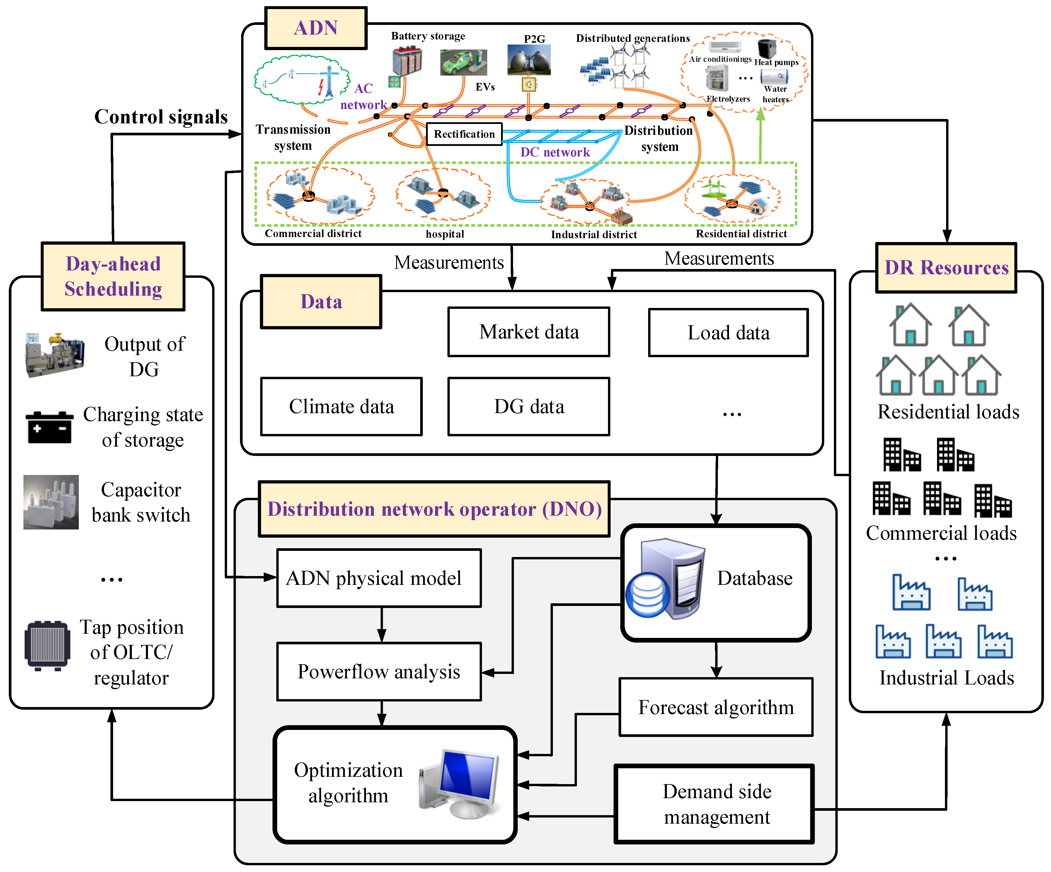
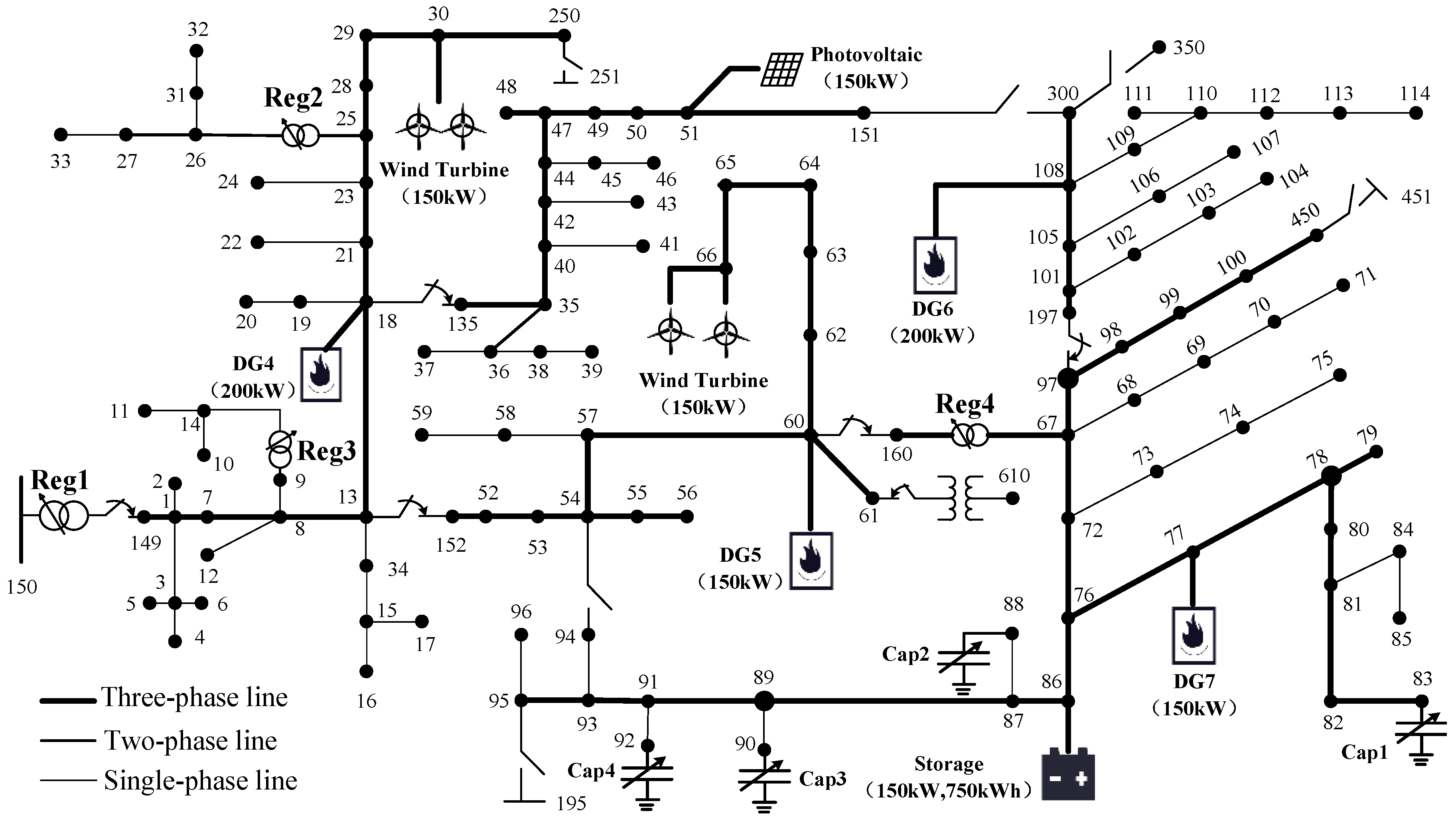
This paper focuses on the optimal scheduling and operation of ADN. The diagram of optimal dispatch for ADN is shown in
Figure 1. As can be observed, there is a diversity of controllable resources in both supply and demand side in ADN, such as regulators, battery storages, DGs, and thermostat controlled loads (TCLs), etc. The distribution network operator (DNO) [
26], which is the control center of ADN, gathers the information from both supply and demand side as well as predicts the scheduling information containing customers’ load profiles and DGs’ outputs. In recent years, with the development of communication and measurement technologies such as advanced metering infrastructure (AMI), the DNO has had the access to acquiring all kinds of necessary information in terms of climate data, market data, and load data. A local database therefore can be constructed, providing data support for the follow-up research. Based on the acquired data and physical model of ADN, the power flow analysis can be accomplished, whose function is to coordinate with the optimization program. Moreover, the scheduling information including the users’ load profiles, output of DGs and so on can be also predicted by using forecast algorithms. Then, based on these information, the optimal dispatch can be achieved by applying the efficient solving algorithm. Finally, the optimal results of ADN for the following scheduling times containing charge/discharge of the battery storages, tap position of regulators and so on can be determined and return to the ADN.
Generally, there are two types of decision variables in distribution network: continuous variables and discrete variables. Continuous variables include power of electric components and node voltage, while discrete variables are characterized by states of devices, such as the operation state of capacitor banks and tap position of voltage regulator or OLTC, etc. Hence, the optimization problem should be formulated as a mixed-integer nonlinear programing (MINP) problem. The objective in this paper is to minimize the power loss of ADN while reducing the fluctuation of nodal voltage profile around the nominal value. The details about the distribution network will be discussed in the fifth part.
2.1. Objective Function
One of the advantages of ADN is that a lot of controllable resources, including DGs, battery storages, voltage regulators as well as switchable capacitor banks can be utilized to achieve the goal of optimal dispatch. In this paper, considering the above resources, the first objective is to minimize the total transmission lines energy losses during the whole schedule time. The first objective function is formulated as follows:
where
is the time interval and in this paper, its value is 1 h; the variable
T represents the scheduling period, which is set to 24 h.
is the total transmission lines active power losses in kW at time
t of ADN. Taking into account the mutual impedance between phases,
can be precisely calculated by Equation (2) [
27]:
In the above equation, and are the real and imaginary part of the voltage at node i of phase at time t, respectively. and are the real and imaginary part of the element corresponding to the γ phase of node i and β phase of node j in the node admittance matrix (). is the collection of all branches.
The second objective function of improving the voltage profiles can be represented by the following equation:
where
is the nominal voltage;
means the voltage magnitude at node
i of phase
p (
) at time
t; and
N is the total node number.
Because the units between the two objectives are inconsistent, it is necessary to normalize
and
. The normalization of the two objective functions can be calculated by:
where
and
is the basic value of normalization and, in this paper, the value of
is the maximum power loss during the day before optimization, while
means the maximum voltage offset during the day before optimization.
Then, a comprehensive objective function
F can be generated after the normalization, reflecting the combined effects of the abovementioned objectives, as Equation (5):
where
and
are the weight coefficients of
and
, respectively. In this paper, the two objectives are considered of equal importance and their value are both 0.5.
2.2. Constraints
The minimization of Problem (5) is subjected to the following constraints (Equations (6)–(20)):
(1) Unbalanced three-phase power flow constraints:
In the following equation, and are the active and reactive generation power injected into node i of phase p, respectively, while and are the corresponding load power at node i of phase p at time t; is the voltage magnitude of phase p at node i and is that of phase m at node j; means the phase angle difference of phase p and m between node i and j; and and represent the real and imaginary parts of admittance matrix, respectively.
(2) Nodal voltage magnitude constraint:
In this paper, the minimum and maximum voltage magnitude are set to 0.95 p.u and 1.05 p.u, respectively.
(3) Constraints of active and reactive power outputs of DGs:
where
and
are the minimum active and reactive power output of DG
n, respectively;
and
are the maximum active and reactive power output of DG
n, respectively; and
and
are the actual active and reactive output of DG
n, respectively. The power generated by DGs is supposed to be assigned to three phases equally.
(4) Thermal limits of transmission lines constraints:
where
is the apparent power of line
l at time interval
t and
represents the maximum transmission power of line
l.
and
are the active and reactive power of line
l at time
t.
(5) Tap change constraints of voltage regulator or OLTC:
where
and
are the lower and upper limit of tap position of regulator
k;
is the actual position at time
t. Equation (12) constraints the actual tap position between
and
. To avoid increasing cost of maintenance caused by changing the tap position frequently, the maximum tap change number constraint, expressed as Equation (13), is introduced during the whole scheduling period, and
means the tap change status at time interval
t.
(6) Switchable capacitor bank switch constrains:
where
is the switch status of capacitor bank
n at time
t, for which 0 represents open and 1 means closed. In addition,
is a logic variable reflecting whether the switch state is changed.
(7) Battery storage constraints:
where
is the charging/discharging power of battery storage
n at time interval
t, for which
means charging and
means discharging;
and
represent the maximum rate for discharge and charge, respectively;
and
mean the allowable range of state-of-charge (SOC), which are 0.2 and 0.95 in this paper; and
represents the charging/discharging efficiency of battery
n. Considering the times of charging/discharging affect the battery life, the charge and discharge times constraint is set in Equation (20), where
means the limit of charge and discharge times and its value is 50 in this paper [
28,
29].
3. Model Solution
In this section, a Kriging model based improved Surrogate Optimization-Mixture-Integer (ISO-MI) algorithm is proposed to solve the optimization problem. The brief introduction of Kriging model is illustrated first. Then, the procedure of the proposed algorithm is explained in detail and, finally, the flowchart of the proposed method is presented.
3.1. Kriging Model
Kriging model is one type of surrogate model; a surrogate model is essentially an approximate model of the complicated physical system, which expresses the relationship between the inputs and the corresponding outputs with simple equation [
30]. Nowadays, there are four kinds of commonly used surrogate models including Response Surface Model (RSM), Kriging models, Radial Basis Function (RBF), and Artificial Neural Network (ANN) [
31]. Every model has its own characteristics and there is no specific criteria to measure which is the best. Many comparative studies have been done and insights have been gained through a number of experiments [
32].
Among these abovementioned models, the Kriging model, combined with a random process, is more accurate for highly nonlinear problems. Besides, Kriging model is also flexible in either interpolating the sample points or filtering noisy data. On the contrary, a polynomial model is easy to construct, clear on parameter sensitivity, and cheap to work with but is less accurate than the Kriging model [
33]. In practical engineering application, Kriging model has been successfully applied in many practical projects, such as structural optimization, airfoil aerodynamic design, missile aerodynamic design, multidisciplinary design optimization and so on. In this paper, considering approximation accuracy and the software tools, the Kriging model is selected to approximate the ADN.
Assume that the sampled points can be expressed by
, and the corresponding response values are
, where
and
can be obtained through history data of ADN. Kriging function combines linear regression model and random process model to predict the real function of the relationship between input and output [
34]. The general form of the Kriging model can be expressed as Equation (21):
where
represents the predictive value of function at point
;
is the polynomial regression function of the sampled points;
denotes the least square estimator of regression coefficients; and
is a Gaussian random process. The detailed calculation process of these variables can be found in [
35] and, in this paper, a MATLAB tool box called DACE [
36] is used to construct the Kriging model.
3.2. Kriging Model Based Optimization
As mentioned above, Kriging model is an approximate model for complex black-box system such as complicated distribution system, it is easy to calculate without losing the approximation accuracy.
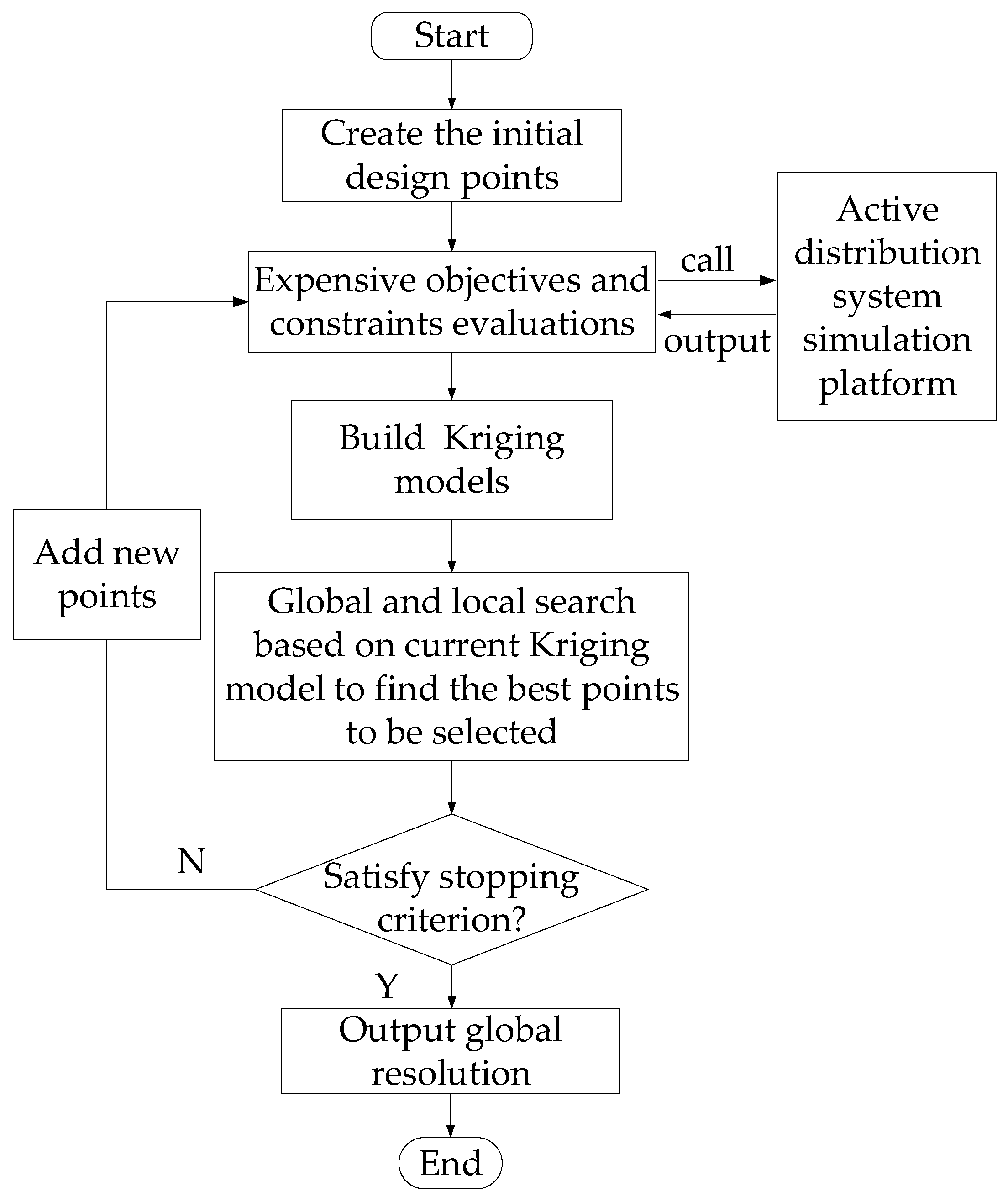
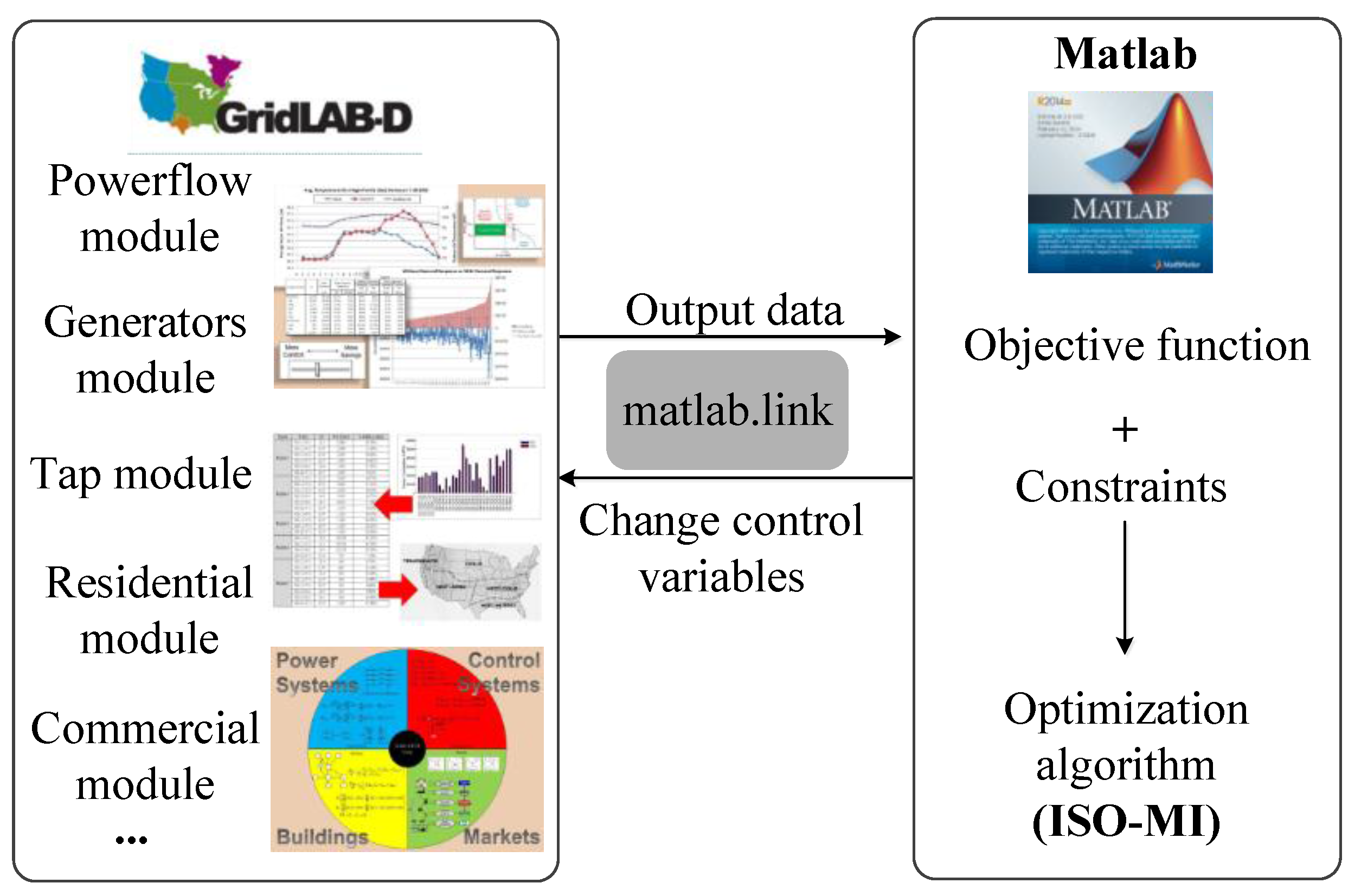
The general framework of Kriging model based optimization algorithm is shown in
Figure 2. To construct Kriging, first, some test points in the decision space should be generated. It is essential to select the design points properly to capture the characteristics of a complicated system. There are two categories of sampling techniques which are the classical techniques and the space filling techniques [
37]. Between the two categories, the latter is widely used to construct Kriging models. The space filling designs include three methods namely Orthogonal arrays, uniform designs and various Latin Hypercube Designs (LHD). Among all of these, LHS is selected because of its good properties of uniformly and flexibility on the size of sampling [
38]. Then the simulation software can be called to compute the actual response of the inputs and outputs. After that, a Kriging model can be constructed by using these experimental data. Finally, the Kriging models can be applied to the solving process of the optimization algorithm under the premise of meeting the approximation accuracy.
In the process of optimization, the Kriging model can be kept constant or dynamically updated. If the model remains unchanged, the initial constructed model is required to meet certain approximation accuracy requirements. However, in the optimization process, the approximation error of the Kriging model is likely to result in an erroneous solution. Therefore, an effective method is to update the constructed model in the process of optimization, so as to improve the approximation accuracy with the model. In this work, the developed optimization algorithm is inspired by the concept of dynamic Kriging model. As shown in
Figure 2, the dynamic Kriging model adopts dynamic adding design point algorithm (DADPA), in which new sample points will be iteratively selected to do the expensive function simulation and update the model until the stopping criterion is met while the whole search space will not be changed. According to [
39], DADPA has good performance in optimization problem.
3.3. Improved Surrogate Optimization-Mixed-Integer Algorithm
Inspired by the optimization algorithm SO-MI (Surrogate Optimization-Mixed-Integer) [
40] developed to solve mixed-integer, no-convex and nonlinear programming problem and DYCORS (Dynamic Coordinate Search Using Response Surface models) framework developed for bound constrained optimization in black-box system [
41], a modified SO-MI named ISO-MI is proposed in this paper to solve the optimal operation and scheduling problem in ADN. Based on the SO-MI, the method of coordinate perturbation is added to improve the efficiency of local search. At the same time, adaptive adjustment strategy of disturbance range is introduced, which balances local and global disturbances and improves the probability of finding better solutions.
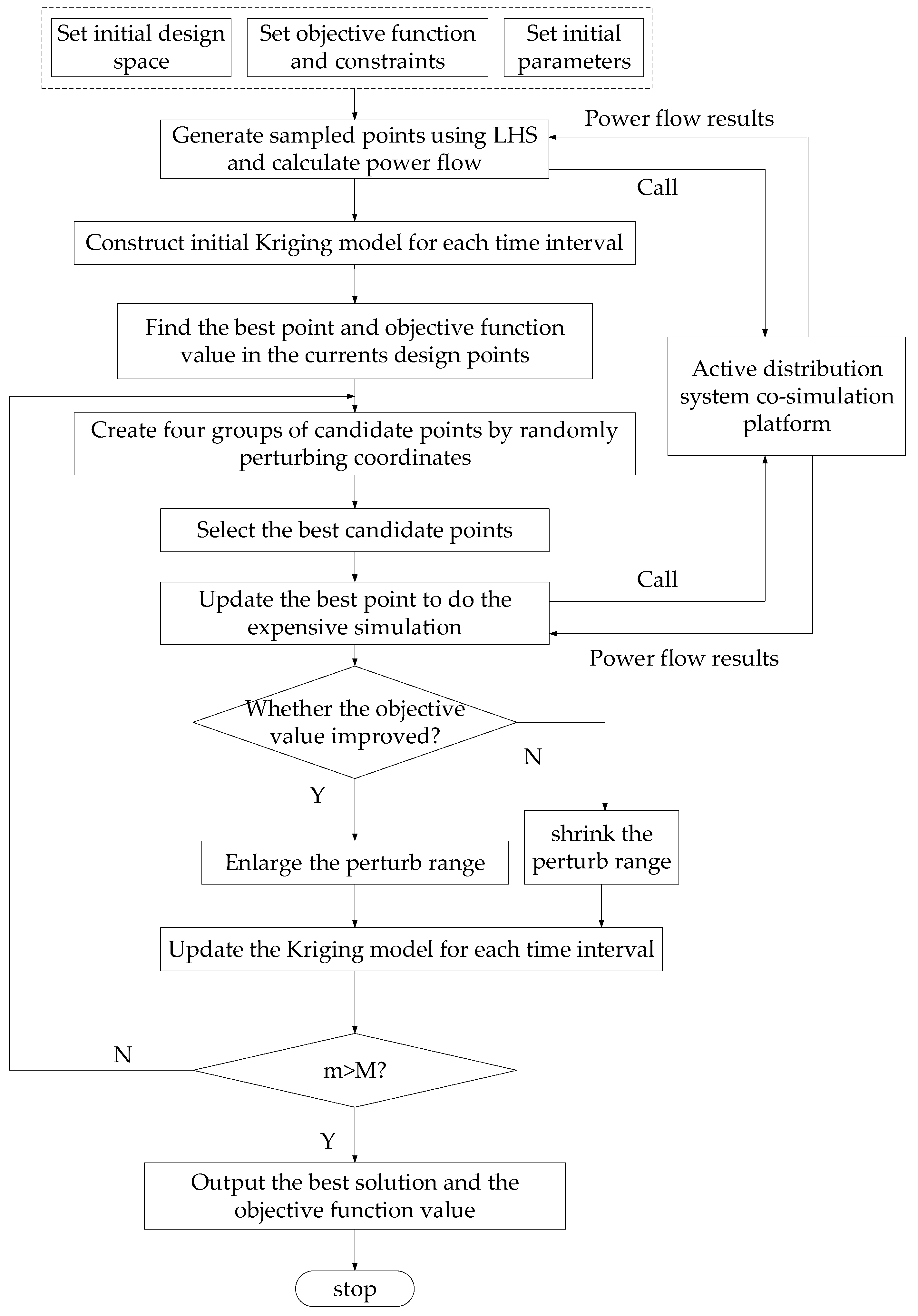
The main procedure of ISO-MI can be divided into four steps and the flowchart of the algorithm is shown in
Figure 3.
Step 1—Construct Initial Kriging model. In this step, it is easy to construct the Kriging model with high accuracy using the measured history operation data of distribution system. denotes the initial surrogate model built by the set of sampled points ;
Step 2—Initialize optimization parameters. In this step, first, a series of parameters need to be set for the beginning of the optimization program, such as maximum evolution number M of expensive simulation, initial coordinate perturbation range and the minimum range , etc. Second, the LHD method is used to generate initial feasible design points. To construct a new Kriging model, it is necessary to do the expensive simulations and get the responses from them. Finally, find the best point , which represents the control variables of the distribution network, and the corresponding objective function value in the current design points.
Step 3—Iterate until the evolution number, m > M, maximum evolution number. In this step, first, create four groups of candidate points by randomly perturbing coordinates around . The purpose is to improve the efficiency of local search by adding the coordinate perturbation. The generation of the four groups in the global range are shown as follows:
- (1)
Group 1: Uniformly and randomly perturb the continuous coordinates of at the range of , , where i is the index of points and ;
- (2)
Group 2: Uniformly and randomly perturb the discrete coordinates of at the range of , ;
- (3)
Group 3: Uniformly and randomly perturb all coordinates of at the range of , and round the discrete coordinates to the closet integers;
- (4)
Group 4: Select candidate points in the whole design space using LHS.
Second, check the candidate points to ensure that they are in feasible domain and discard the points that violate the constraints. Third, select the best candidate points from four groups of candidate points. The specific method is illustrated as follows:
- (1)
Calculate the objective function using the initial Kriging model and current new Kriging model of candidate points in four groups and compute the objective function score and of all points, where and are the normalized objective functions. Their value can be calculated by Euclidean distance in n dimensional space.
- (2)
Compute the distance score of all design points.
- (3)
Compute the weighted score , where denotes the objective function F in this paper, and select the point with minimum score to add it into design points set and do the expensive function evaluation, again.
Fourth, update the best point and corresponding objective function value in the current design points set , where is the sub-objective function. Fifth, check if the objective function value has an improvement (). If this is true, the perturb range should be enlarged to two times. Otherwise, it will be shrink for the purpose of balancing the local and global search. Finally, update the current Kriging model.
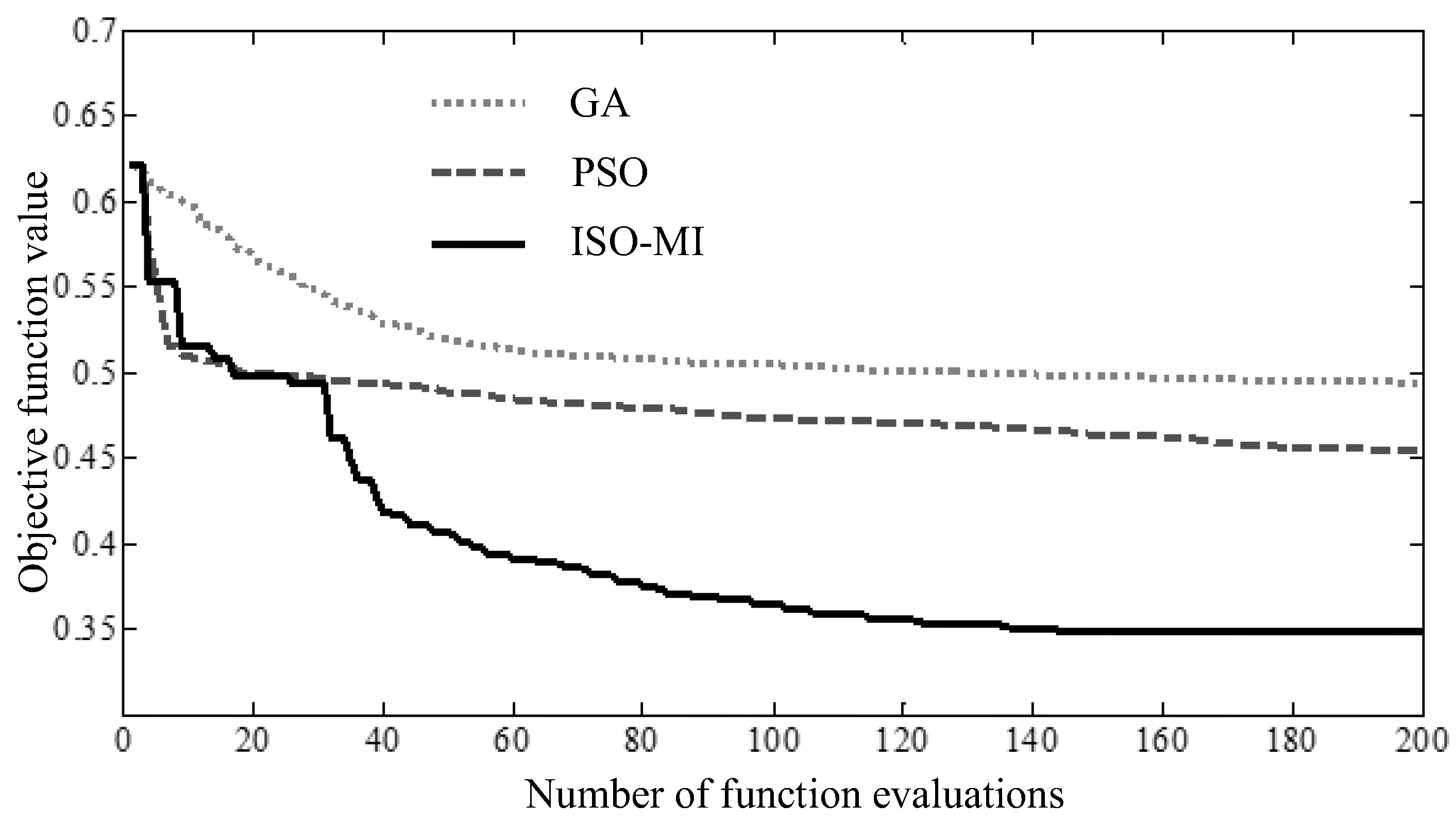
Step 4—Output the value of best solution and the corresponding objective functions found so far.


