Comparative Performance Analysis of Optimal PID Parameters Tuning Based on the Optics Inspired Optimization Methods for Automatic Generation Control


1
Electrical and Electronics Engineering, Faculty of Engineering, Fırat University, 23100 Elazığ, Turkey
2
Department of Electrical and Electronics, Faculty of Engineering and Architecture, Bingöl University, 12000 Bingöl, Turkey
*
Author to whom correspondence should be addressed.
Energies 2017, 10(12), 2134; https://doi.org/10.3390/en10122134
Submission received: 17 October 2017
/
Revised: 6 December 2017
/
Accepted: 11 December 2017
/
Published: 14 December 2017
(This article belongs to the Section F: Electrical Engineering)
Abstract
:The Optics Inspired Optimization (OIO) algorithm is a new metaheuristic optimization method. In this paper, the OIO algorithm was proposed for automatic production control parameters in electrical power systems. The performance of the proposed algorithm was realized on two power systems that have different structures. The first structure is a two-area interconnected thermal reheat power system and the other one is a two-area interconnected multi-unit hydro-thermal power system. The results obtained with the proposed algorithm were compared with an artificial bee colony and particle swarm optimization, initial values are randomly defined that are commonly used in literature. The results were examined using four different cost functions based on area control error. Considering the obtained results, the proposed algorithm reached to the global minimum value with less number of iterations and is more suitable for online optimization. According to the results obtained with this novel method, it has a better performance for maximum overshoot and settling time values when the test systems are implemented.
1. Introduction
The amount of electrical energy consumed per person shows the level of development of a country and the quality of this energy consumed by people is also an important criterion. The system frequency and voltage are the two most important parameters that determine the power quality. Controlling the frequency takes longer than controlling the voltage and it is a more dominant parameter in the power system. Therefore, the primary parameter that should be controlled is frequency [1]. The interconnected power system is created by integration of many areas. Any power changes (supply or demand) that will occur in any of these areas will affect other areas that are connected in terms of frequency and power. In addition, characteristic of the connecting line between the areas connected to the power system is another factor affecting the frequency change. When changes in the frequency of the power system exceeds the limits set, they may create serious instability problems in electrical power system, stop of the plants connected to the system and even black-out of the system at later stages. In such a case, the area feeding from the system will remain de-energized and there will be huge economic losses. Black-outs affected 77 million people in 2015 in Turkey, 150 million people in 2014 in Bangladesh and 620 people in 2012 in India some examples of these huge losses [2]. Therefore, considering these huge economic losses caused by system failures, the load-frequency control is a crucial issue that should be taken into consideration in order to prevent such losses.
Behaviors of systems/living creatures such as nature, society, culture, politics, and human have been the source of inspiration of most of the algorithms created from the 1970s until today. Metaheuristic is used for combination of randomness and rules of natural phenomena that are imitated. In recent years, metaheuristic methods have attracted the attention of researchers in many disciplines.
This interest has increased further with the implementation of the actual optimization problems particularly in engineering applications and many other industrial areas. Different metaphors are used for search processes of each metaheuristic optimization. For example, particle swarm optimization algorithm, that is called the PSO in literature, introduced by Eberhart in 1995, models herd behavior of birds [3]; harmony search algorithm, called the HAS, introduced by Geem et al. in 2001, searches for the perfect harmony by using the musical process [4]; bacteria foraging optimization algorithm, called the BFOA, introduced by Passino and Biomimicry in 2002, models the process of the search of a single bacteria for food with the lowest energy [5]. The bacteria chemotaxis algorithm, called the BC, introduced by Muller et al. in 2002, shows reaction tendency of bacteria towards chemical agents in the concentration trend [6]. The artificial bee colony algorithm, called the ABC, proposed by Karaboğa in 2005, simulates foraging behaviors of honey bee swarms [7]. The center power optimization algorithm, called the CFO, proposed by Formato in 2007, makes an analogy between the search operation in the decision space for maximum value of objective function and moving searches along the physical space under the effect of gravity [8].
The firefly algorithm, called the FA, proposed by Yang in 2010, is performed based on idealization of light emission characteristics of fireflies [9]. The league championship algorithm, called the LCA, introduced by Kashan in 2009, is based on simulating league games with modelling game analysis methods using experiences of the coaches [10]. The group search optimization, called the GSO, introduced by He et al. in 2009, simulates search behaviors of animals such as feeding, breeding, egg spread and nidification [11]. The gravitational search algorithm, called the GSA, announced by Rashedi et al. in 2009, was established based on the concept of mass interactions and the law of gravity [12]. The teaching-learning based optimization, called the TLBO, announced by Rao et al. in 2011, imitates the teaching-learning process in the classroom between teachers and students [13]. Krill herd algorithm, called the KH, announced by Gandomi et al. in 2012, works by performing simulations of gathering krill swarms together in response to specific biological and environmental processes [14].
Optimization methods have been applied to many problems in power systems such as automatic voltage regulation [15], load frequency control [15,16,17,18,19,20], and optimal power flow [21,22,23]. In the power systems, conventional proportional integral derivative controls (PID) are widely used for Automatic Generation Control. Many studies were conducted to determine the best PID parameters. Metaheuristic methods Bacteria Foraging [24,25,26,27], PSO [28,29,30,31,32,33], Ant Colony Optimization [34], Artificial Bee Colony [35] and Orthogonal Learning Artificial Bee Colony [36] are used in the determination of controller gains. Although these methods seem to be good methods for determining the controller gains, they have problems such as slow convergence and local minimums in the step of global minimum search. Optics inspired optimization (OIO), which is a new metaheuristic method, is found to be showing better performance in terms of these aspects [37,38].
In the literature, the main aim of the current study is to design and implement a new metaheuristic method for optimal design of a PID controller to solve an LFC problem. In this paper, the OIO algorithm was proposed in order to identify the optimal PID controller parameters which is controlling the frequency of an electrical power systems. For this purpose, two different test systems were investigated and named as test system-1 and test system-2 in this paper. The rest of the paper is organized as follows:
Section 1 discusses how PID controller gains were determined by using OIO, PSO, ABC, and other heuristic algorithms in literature and their performances were compared to each other. In Section 2, the mathematical model and block diagram of a two-area test power systems are given. In Section 3, the proposed OIO optimization method is discussed. In Section 4, the integral of squared error (ISE), the Integral of absolute error (IAE), the integral of time multiply squared error (ITSE) and the integral of time multiply absolute error (ITAE) cost functions were used as the performance index. Frequency changes in the two regions and simulation results of the power variation of collection line is obtained for each performance index. Finally, we discuss conclusions in Section 5.
2. Power System Model
Potential/Kinetic energy is converted into mechanical energy by means of turbines and then the mechanical energy is converted into electrical energy via generators in a power plant, which has rotating machines. The simplified equation of motion belonging to this principle is written:
where, is mechanical momentum, is load moment, J is the moment of inertia, and ω is angular velocity.
An interconnected power system consists of areas connected to each other with tie-line. It is assumed that generator groups, which exist in each of the areas, have a composite structure. The frequency deviations can occur in some areas of the power system. Deviations cause a variation in power flow in the tie-line. In the present case, the variation and area frequency are required to be controlled. Each area provides its own users with energy and the tie-line allows inter-area power flow. Therefore, when there is a sudden load change in an area, frequency in other areas and power flow in tie-lines are affected. Controllers need information about the transient state of each area to return the system to the required steady state. Thus, it could return frequency of the system to the required steady state. If losses in the tie-line are ignored, the power flow in the tie-line can be written as:
where V1 and V2 are voltage amplitude of the first and second areas, respectively, Δ1 and Δ2 are corresponding phase angles, and X12 is the impedance of the tie-line between the two areas. Where the phase angle deviation for each area is written as:
Power flow deviation between areas will be:
where the synchronizing moment coefficient of the tie-line is:
When the moment coefficient is written in its place in (4), the power deviation of the tie-line will be:
In consequence of power deviation, of the system, frequency deviation, power deviation, and control error (Area Control Error—ACE) are as follows:
Block diagram of the test system-1 and test system-2 are depicted in Figure 1.
Transfer function of each block is given below:
Governors:
Re-heater:
Turbine:
Valve:
Power system:
Tie-line:
Test system-1 [39,40] and test system-2 [41,42] are widely employed in literature. System parameters used for test system-1 and test system-2 are given below:
Parameters of Test System-1:
Rating of each area = 2000 MW, base power = 2000 MVA, f = 60 Hz, Pr1 = Pr2 = 1000 MW, Kg = 120 Hz/p.u. MW, Tg = 20.0 s, Kr12 = 0.5, Tr1 = Tr2 = 10.0 s, Tg1 = Tg2 = 0.086 s, Tt1 = Tt2 = 0.3 s, R1 = R2 = 2.43 Hz/p.u. MW, B1 = B2 = 0.425 p.u. MW/Hz, a12 = −1, T12 = 0.0707, ΔPL1 = 0.01 p.u. MW.
Parameters of Test System-2:
Rating of each area = 2000 MW, base power = 2000 MVA, f = 50 Hz, Pr1 = Pr2 = 1000 MW, K2_h = 1, T2_h = 48.7 s, K2_1h = 1, T2_1h = 0.08 s, Kst2 = 1, T2t = 0.3 s, Tvr = 5 s, Tv2 = 0.513 s, Tw = 1 s, R2_11 = R2_21 = 2 Hz/p.u. MW, R2_1 = R2_2 = 2.4 Hz/p.u. MW, Kg_2 = 100, Tg_2 = 20 s, B2_1 = B2_2 = 0.425 p.u. MW/Hz, a2_12 = −1, T2_12 = 0.0707 s.
3. Optics Inspired Optimization
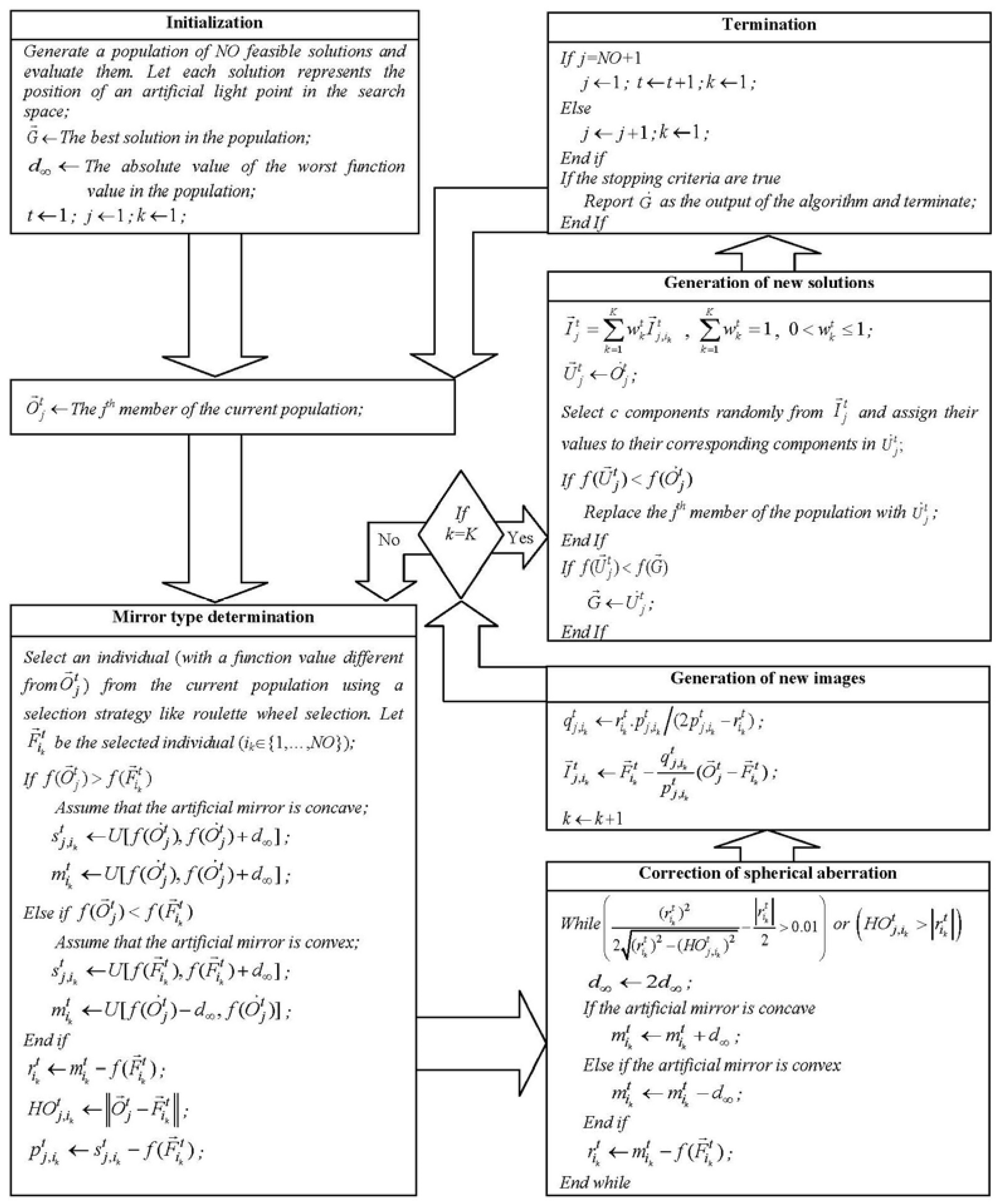
OIO algorithm is a physics-based heuristic algorithm introduced by Ali Husseinzadeh Kashan in 2014 [38]. It was developed by being inspired from optics, which is one of the laws of physics. OIO is an algorithm assuming that there are a series of artificial light points (points at Rn+1 matching at Rn are potential solutions to the problem) of an artificial mirror reflecting the image. Each bump is accepting as a convex reflecting surface and each concave is considered as a concave reflecting surface. In this way, an artificial light coming from an artificial light point is reflected back from the function surface of a part of convex or convey surface. Artificial image point (like a new solution in the search area at Rn+1 matching at Rn) is either straight (in the direction of position of light point in the search space) or reverse (outward from position of light point in the search space).
is a numerical function that can be minimized with n variables in the n-dimensional decision space defined with , d = 1,… ni. Let’s remember that we are looking for the general minimum of f finding where for .
It should be noted that common search and objective space is a vector in and it is a subset of .
- -
- indicates the position of j artificial point of light in the t iteration and n-dimensional space (i.e., j th solution in the population).
- -
- specifies a different point in the search space passing through its own artificial axis (an individual in position). Artificial mirror peak position is determined by vector. index is randomly selected from NO is the number of artificial light points.
- -
- specifies location of an image of j artificial point of light in the t iteration in the search space. The artificial image is created through by an artificial mirror passing through the main axis.
- -
- specifies the position of j artificial light point on function/objective axis (objective space) in t iteration. The position of j artificial light point in common search and objective space is given by vector.
- -
- is the distance between j artificial light point on function/objective axis (objective space) and vertex of the artificial mirror in t iteration.
- -
- is the distance between j artificial light point on function/objective axis and position of vertex of the artificial mirror on function/objective axis .
- -
- is the radius of curvature of an artificial mirror that can pass through the center of curvature of an artificial mirror on the main axis through .
- -
- is the position of the center of curvature on function/objective axis (in the objective space).
- -
- is the height of j artificial light point from the artificial main axis in t iteration.
- -
- is the height of image of j artificial light point from the artificial main axis in t iteration.
- -
- is the value of lateral deviation on artificial mirror reflecting the image of j artificial light point in t iteration.
It is possible to express the general mechanism of the OIO as follows: first, NO individuals are randomly generated to create the initial positions of artificial light points in the search space; then, each j artificial light point in the search space of t iteration and is put in front of the artificial mirror with a distance of from the corner of the mirror (in the common search and objective space positioned at and its artificial image is created in the search and objective space with a distance of from the main axis (on function/objective axis) where point passes the axis ( is randomly selected from the population in case differs from . The radius of curvature of the artificial mirror is . The position of the artificial image is produced by an artificial image position that can be a new solution to the problem in the search space by matching with the solution space. The flow chart of OIO algorithm is shown in Figure 2.
4. Results
In the simulations, the power change occurred in the connection line while frequency change occurred in two areas in response to a ∆PL1 change in the first area is costed by using various performance indices that are ISE, IAE, ITAE, and ITSE. The mathematical expressions are shown below.
- Integral of square error (ISE)
- Integral of absolute value of error (IAE)
- Time-weighted ITAE
- Time-weighted ITSE
In the simulations, the results of power change occurred in the connection line while frequency change occurred in two areas in response to a change of at t = 0 are given in tables and time domain simulations. The controller parameters used in the results are determined according to OIO, PSO, and ABC. The model created and m files are performed in MATLAB R2013a. The lower and upper limits of Kp, Ki, and Kd values, which are the controller gains, are given in Table 1.
The controller parameters optimized by four different performance indices with the limitations seen in Table 1 are given in Table 2.
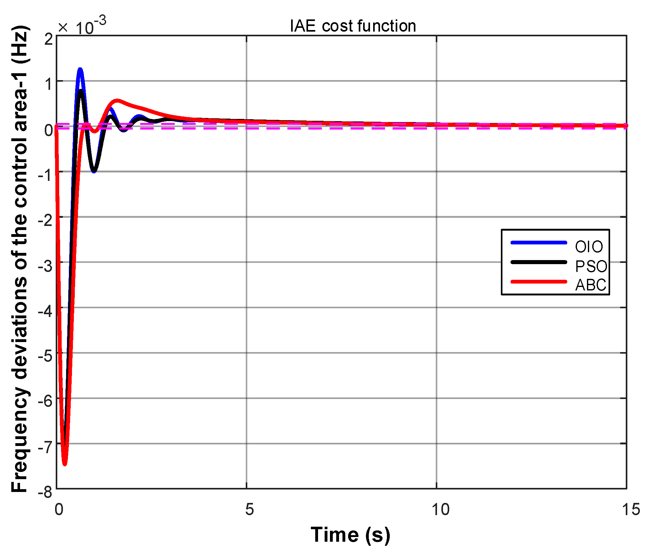
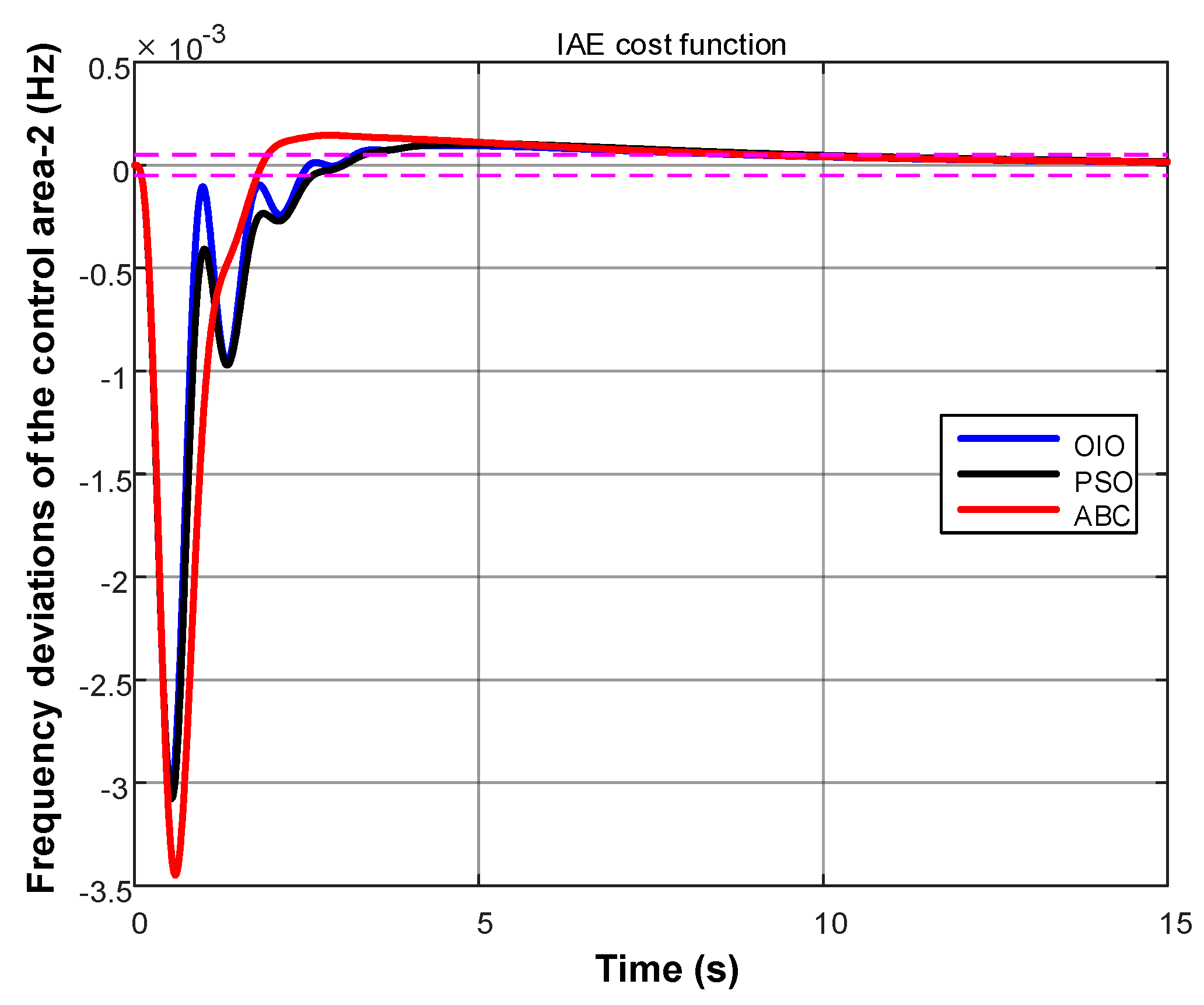
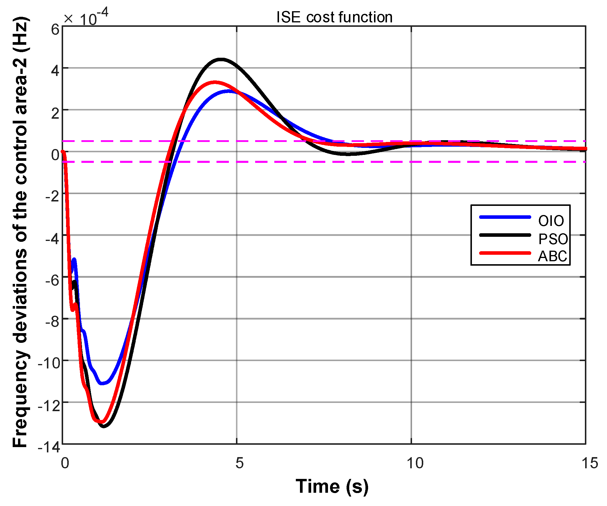
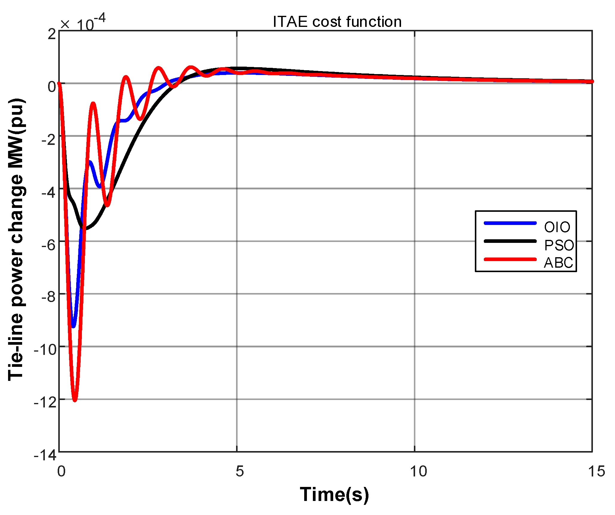
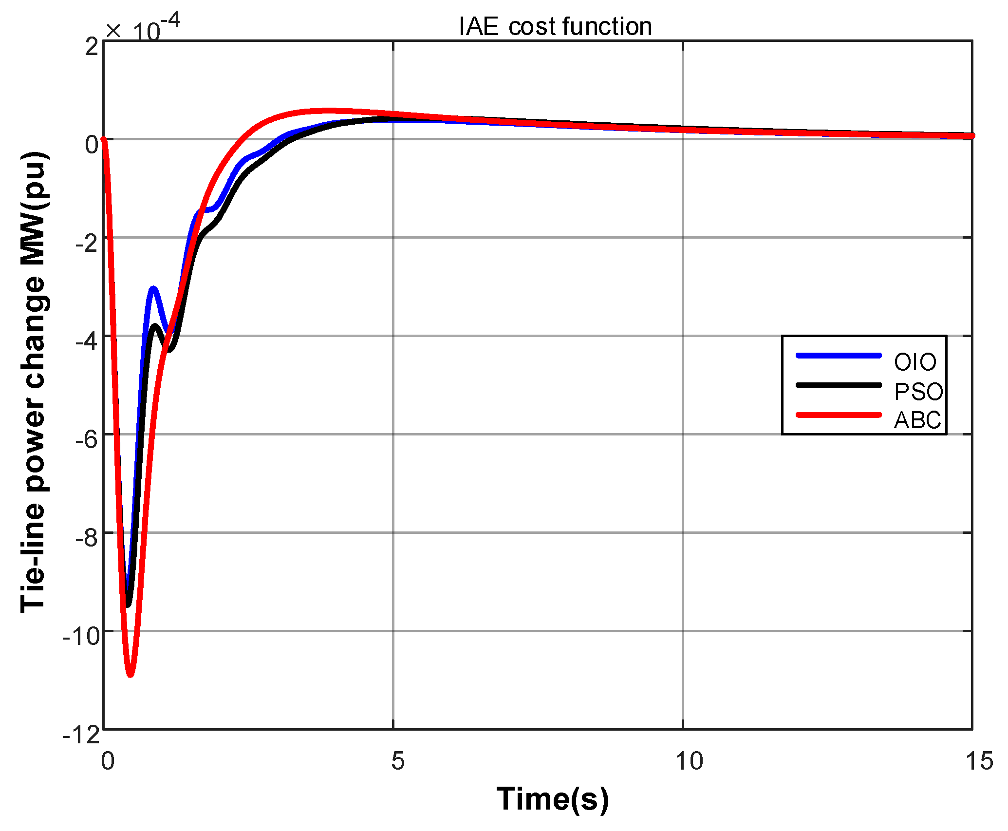
The time domain simulation results, Figure 3 and the following 14 figures, are given only for test system-1. Similar results are not given for test system-2. However, the performances of all simulation results are given with all tables Table 2 and the following 4 tables. In Figure 3, Figure 4, Figure 5 and Figure 6, the frequency changes occurred in the first area as a result of the simulation performed with controller parameters optimized for ITAE, IAE, ISE, and ITSE performance indices are shown. The frequency changes of the second area are given in Figure 7, Figure 8, Figure 9 and Figure 10. In Figure 11, Figure 12, Figure 13 and Figure 14, the power change in the connecting line is given. The maximum overshoot and settlement times are given in Table 3 and Table 4 according to the time-domain simulations.
Figure 3, Figure 4, Figure 5, Figure 6, Figure 7, Figure 8, Figure 9, Figure 10, Figure 11, Figure 12, Figure 13 and Figure 14 are given data with the aim of better illustrating the data given in Table 3 and Table 4 which are the tables that include maximum overshoot and settling time in every area. In these tables when the results of test system-1 are considered, apparently it is seen that OIO gives better result for maximum overshoot and settling times. In the first area, the best result was obtained with PSO in terms of the maximum overshoot for ITAE performance index, whereas the best settlement result was obtained by OIO method. According to settling time values while the best results are found with the help of OIO for IAE, ITSE, and ITAE values, PSO found better results for ISE. The results of the second area are similar with the results of the first area.
As the results of test system-2 are considered, apparently it is seen that OIO gives better result for maximum overshoot and settling times. In the first area, the best result was obtained with PSO in terms of the maximum overshoot for ISE performance index, whereas the best settlement result was obtained by OIO method. According to settling time OIO is the best result for ISE and ITAE and PSO becomes prominent for ITSE and ISE. The results of the second area are similar with the results of the first area.
The best results are obtained with OIO method in both first and second areas in maximum overshoot and settling times for IAE, ISE, and ITSE performance indices.
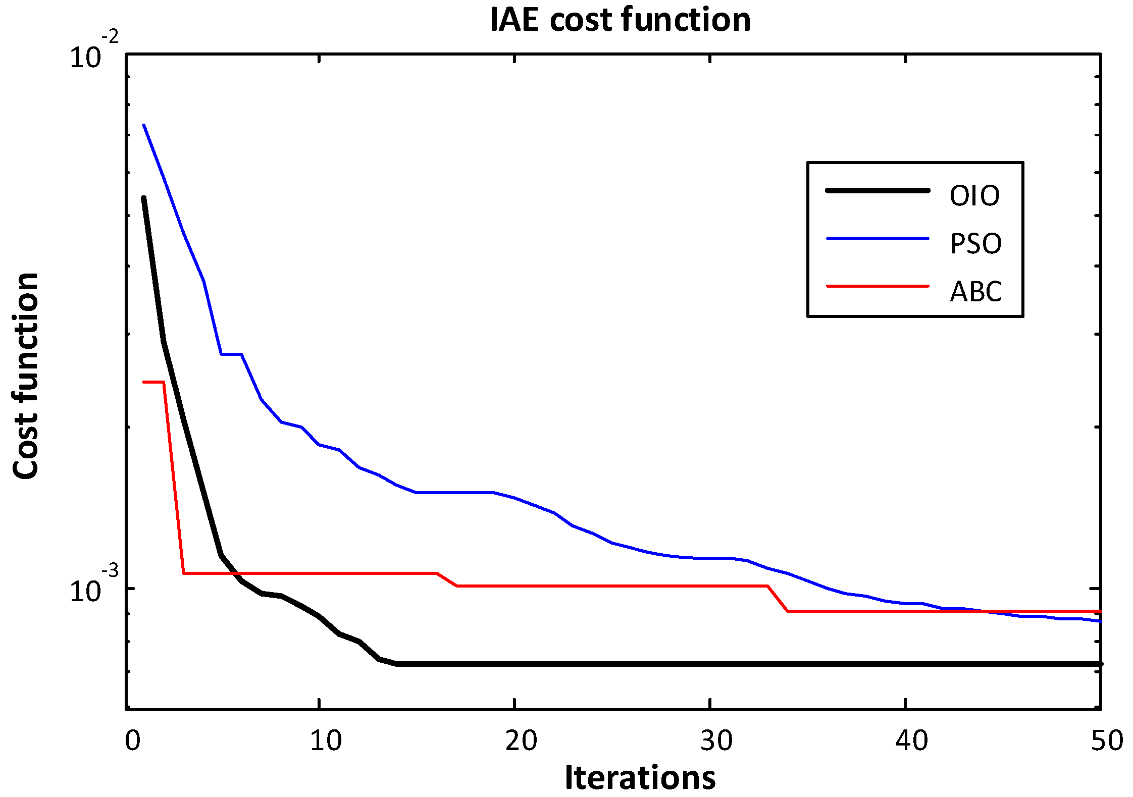
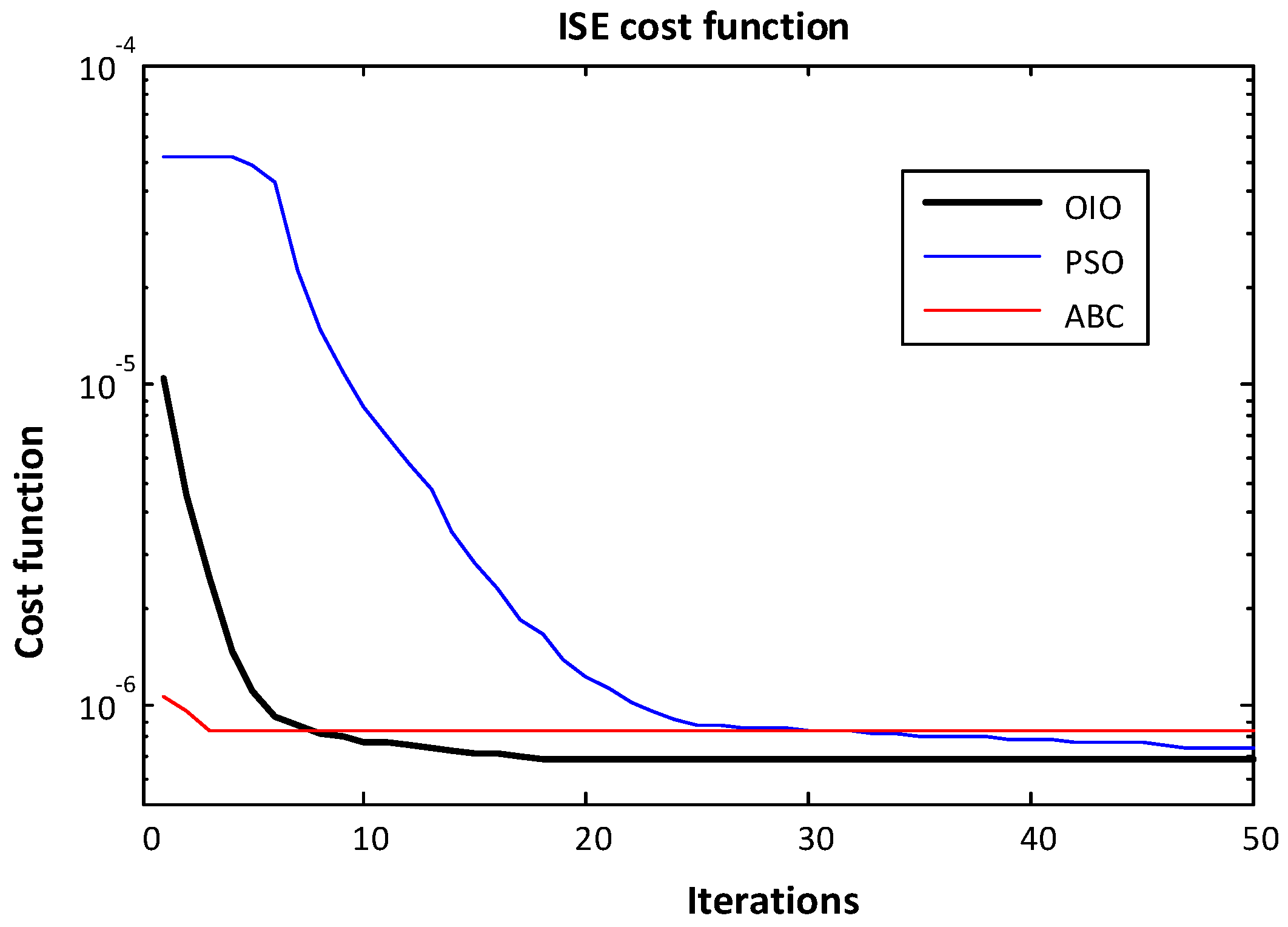
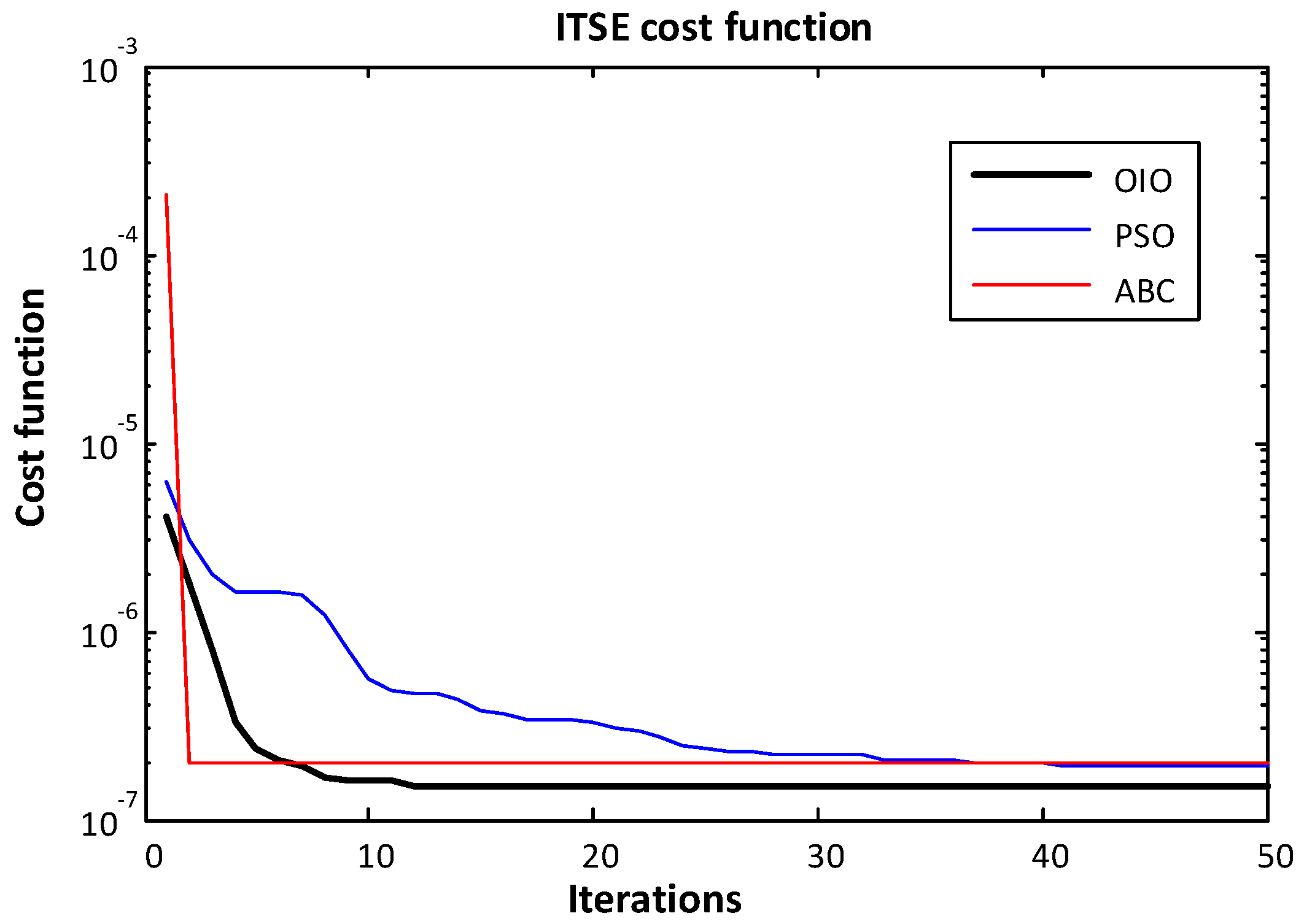
In Figure 15, Figure 16, Figure 17 and Figure 18. The change of cost function values for four different performance indices are given for Test system-1 and Figure 19, Figure 20, Figure 21 and Figure 22. For Test system-2. The final values of these changes are shown in Table 5. Considering these figures and the data given in tables. It is clearly seen that OIO algorithm finds smaller values earlier than other methods.
Total optimization times for each method and algorithm are given in Table 6. OIO algorithm realized optimization process in a shorter time for both test systems. The number of mirror used in OIO algorithm corresponds to the number of population. The number of mirror was specified as 2 in implemented optimizations. The number of population for artificial bee colony for is 3 and 4 for particle swarm optimization. When the number of population is decreased it is seen that the methods occur to have the problem of convergence. All parameters used in all three algorithms are presented in Appendix A.
In Figure 19, Figure 20, Figure 21 and Figure 22 optimization histories are given for test system-2. Although the ABC algorithm has a higher convergence speed, it is seen that it cannot find global minimum. When time domain results and Table 5 are considered, the speed of convergence and reached global minimum values for OIO algorithm are better.
5. Conclusions
In this paper, the OIO algorithm was proposed for optimizing controller gains in load frequency controls in electrical power systems. The reason to use the method developed by Kashan is that it reaches the global minimum value faster. The method was compared with PSO and ABC methods which are widely used in literature. The idea behind choosing these methods is that their initial conditions are randomly defined. These three methods were optimized with two different test systems and four different cost functions. According to the results obtained, OIO algorithm converges to the global minimum value with ten iterations in average. The results obtained from these two test systems can be ordered as follows:
- OIO algorithm has found lowest cost value.
- OIO algorithm reaches to the global minimum value in short time.
- OIO can converge with less number of population.
- OIO algorithm has the total lowest optimization time.
As the authors conclude from the results explained above, they propose OIO algorithm in specifying PID gains online for a two-area power systems in laboratory applications for future studies.
Author Contributions
Mahmut Temel ÖZDEMİR proposed the novel idea behind this work, designed the algorithm framework, and prepared manuscript; Dursun ÖZTÜRK performed the simulations for the two area test systems models, analyzed the simulation results, improve the language. Both authors approved the final manuscript.
Conflicts of Interest
The authors declare no conflict of interest.
Appendix A
OIO
NO = 2 population size; step number = 100 (test system-1)/50 (test system2)
ABC
nPop = 3 population size; iter number = 100 (test system-1)/50 (test system2)
PSO
n = 4 Size of the swarm; bird_setp = 100 (test system-1)/50 (test system2); c2 = 1.2 PSO parameter C2; c1 = 0.12 PSO parameter C1; w = 0.9 Inertia weight
References
- Kundur, P. Power System Control and Stability; McGraw-Hill: New York, NY, USA, 1994. [Google Scholar]
- Özdemir, M.T.; Öztürk, D.; Eke, İ.; Çelik, V.; Lee, K. Tuning of Optimal Classical and Fractional Order PID Parameters for Automatic Generation Control Based on the Bacterial Swarm Optimization. IFAC-PapersOnLine 2015, 48, 501–506. [Google Scholar] [CrossRef]
- Eberhart, R.; Kennedy, J. A new optimizer using particle swarm theory. In Proceedings of the Sixth International Symposium on Micro Machine and Human Science (MHS ’95), Nagoya, Japan, 4–6 October 1995; pp. 39–43. [Google Scholar]
- Geem, Z.; Kim, J.; Loganathan, G.V. A New Heuristic Optimization Algorithm: Harmony Search. Simulation 2001, 76, 60–68. [Google Scholar] [CrossRef]
- Passino, K.M. Biomimicry of bacterial foraging for distributed optimization and control. IEEE Control Syst. Mag. 2002, 22, 52–67. [Google Scholar] [CrossRef]
- Muller, S.D.; Marchetto, J.; Airaghi, S.; Kournoutsakos, P. Optimization based on bacterial chemotaxis. IEEE Trans. Evol. Comput. 2002, 6, 16–29. [Google Scholar] [CrossRef]
- Karaboga, D. An Idea Based on Honey Bee Swarm for Numerical Optimization; Technical Report TR06; Erciyes University: Kayseri, Turkey, 2005. [Google Scholar]
- Formato, R.A. Central Force Optimization: A New Metaheuristic with Applications in Applied Electromagnetics. Prog. Electromagn. Res. 2007, 77, 425–491. [Google Scholar] [CrossRef]
- Yang, X.S. Firefly algorithm, stochastic test functions and design optimization. Int. J. Bio-Inspir. Comput. 2010, 2, 78–84. [Google Scholar] [CrossRef]
- Kashan, A.H. League Championship Algorithm: A new algorithm for numerical function optimization. In Proceedings of the International Conference of Soft Computing and Pattern Recognition (SoCPaR 2009), Malacca, Malaysia, 4–7 December 2009; pp. 43–48. [Google Scholar]
- He, S.; Wu, Q.H.; Saunders, J.R. Group search optimizer: An optimization algorithm inspired by animal searching behavior. IEEE Trans. Evol. Comput. 2009, 13, 973–990. [Google Scholar] [CrossRef]
- Rashedi, E.; Nezamabadi-Pour, H.; Saryazdi, S. GSA: A Gravitational Search Algorithm. Inf. Sci. 2009, 179, 2232–2248. [Google Scholar] [CrossRef]
- Rao, R.V.; Savsani, V.J.; Vakharia, D.P. Teaching–learning-based optimization: A novel method for constrained mechanical design optimization problems. Comput.-Aided Des. 2011, 43, 303–315. [Google Scholar] [CrossRef]
- Gandomi, A.H.; Alavi, A.H. Krill herd: A new bio-inspired optimization algorithm. Commun. Nonlinear Sci. Numer. Simul. 2012, 17, 4831–4845. [Google Scholar] [CrossRef]
- Lu, Q.-Y.; Hu, W.; Zheng, L.; Min, Y.; Li, M.; Li, X.; Ge, W.; Wang, Z. Integrated Coordinated Optimization Control of Automatic Generation Control and Automatic Voltage Control in Regional Power Grids. Energies 2012, 5, 3817–3834. [Google Scholar] [CrossRef]
- Muñoz-Benavente, I.; Gómez-Lázaro, E.; García-Sánchez, T.; Vigueras-Rodríguez, A.; Molina-García, A. Implementation and Assessment of a Decentralized Load Frequency Control: Application to Power Systems with High Wind Energy Penetration. Energies 2017, 10, 151. [Google Scholar] [CrossRef]
- Song, J.; Pan, X.; Lu, C.; Xu, H. A Simulation-Based Optimization Method for Hybrid Frequency Regulation System Configuration. Energies 2017, 10, 1302. [Google Scholar] [CrossRef]
- Huang, C.; Yue, D.; Xie, X.; Xie, J. Anti-Windup Load Frequency Controller Design for Multi-Area Power System with Generation Rate Constraint. Energies 2016, 9, 330. [Google Scholar] [CrossRef]
- Mohanty, B. TLBO optimized sliding mode controller for multi-area multi-source nonlinear interconnected AGC system. Int. J. Electr. Power Energy Syst. 2015, 73, 872–881. [Google Scholar] [CrossRef]
- Zeng, G.-Q.; Xie, X.-Q.; Chen, M.-R. An Adaptive Model Predictive Load Frequency Control Method for Multi-Area Interconnected Power Systems with Photovoltaic Generations. Energies 2017, 10, 1840. [Google Scholar] [CrossRef]
- Surender, R.S.; Srinivasa Rathnam, C. Optimal Power Flow using Glowworm Swarm Optimization. Int. J. Electr. Power Energy Syst. 2016, 80, 128–139. [Google Scholar] [CrossRef]
- Reddy, S.S. Solution of multi-objective optimal power flow using efficient meta-heuristic algorithm. Electr. Eng. 2017. [Google Scholar] [CrossRef]
- Surenderr, R.S.; Bijwe, P.R.; Abhyankar, A.R. Faster evolutionary algorithm based optimal power flow using incremental variables. Int. J. Electr. Power Energy Syst. 2014, 54, 198–210. [Google Scholar] [CrossRef]
- Ali, E.S.; Abd-Elazim, S.M. Bacteria foraging optimization algorithm based load frequency controller for interconnected power system. Int. J. Electr. Power Energy Syst. 2011, 33, 633–638. [Google Scholar] [CrossRef]
- Saikia, L.C.; Nanda, J.; Mishra, S. Performance comparison of several classical controllers in AGC for multi-area interconnected thermal system. Int. J. Electr. Power Energy Syst. 2011, 33, 394–401. [Google Scholar] [CrossRef]
- Özdemir, M.T.; Öztürk, D. Optimal Load frequency control in two area power systems with Optics Inspired Optimization. Firat Universitesi Muhendislik Bilimleri Dergisi 2016, 2, 57–66. [Google Scholar]
- Muñoz, M.A.; Halgamuge, S.K.; Alfonso, W.; Caicedo, E.F. Simplifying the bacteria foraging optimization algorithm. In Proceedings of the 2010 IEEE Congress on Evolutionary Computation (CEC), Barcelona, Spain, 18–23 July 2010. [Google Scholar]
- Yousuf, M.S.; Al-Duwaish, H.N.; Al-Hamouz, Z.M. PSO based single and two interconnected area predictive automatic generation control. WSEAS Trans. Syst. Control 2010, 5, 677–690. [Google Scholar]
- Gozde, H.; Taplamacioglu, M.C. Automatic generation control application with craziness based particle swarm optimization in a thermal power system. Int. J. Electr. Power Energy Syst. 2011, 33, 8–16. [Google Scholar] [CrossRef]
- Serbet, F.; Kaya, T.; Ozdemir, M.T. Design of digital IIR filter using Particle Swarm Optimization. In Proceedings of the 2017 40th International Convention on Information and Communication Technology, Electronics and Microelectronics, Opatija, Croatia, 22–26 May 2017. [Google Scholar]
- Panda, S.; Mohanty, B.; Hota, P.K. Hybrid BFOA–PSO algorithm for automatic generation control of linear and nonlinear interconnected power systems. Appl. Soft Comput. 2013, 13, 4718–4730. [Google Scholar] [CrossRef]
- Özdemir, M.T.; Yildirim, B.; Gülan, H.; Gençoğlu, M.T.; Cebeci, M. Automatic Generation Control in an AC Isolated Microgrid using the League Championship. Fırat Üniversitesi Mühendislik Bilimleri Dergisi 2017, 29, 109–120. [Google Scholar]
- Özdemir, M.T.; Yıldız, S. Effects of High Voltage Direct Current Transmission Lines on Load Frequency Control in a Multi Area Power System. In Proceedings of the Güç Sistemleri Konferansı, Istanbul, Turkey, 15–16 November 2016; pp. 1–5. [Google Scholar]
- Hsiao, Y.; Chuang, C.; Chien, C. Ant colony optimization for designing of PID controllers. In Proceedings of the 2004 IEEE International Conference on Robotics and Automation, New Orleans, LA, USA, 2–4 September 2004; IEEE Cat. No.04CH37508. pp. 321–326. [Google Scholar]
- Naidu, K.; Mokhlis, H.; Bakar, A.H.A. Multiobjective optimization using weighted sum Artificial Bee Colony algorithm for Load Frequency Control. Int. J. Electr. Power Energy Syst. 2014, 55, 657–667. [Google Scholar] [CrossRef]
- Eke, İ.; Taplamacıoğlu, M.C.; Lee, K.Y. Robust Tuning of Power System Stabilizer by Using Orthogonal Learning Artificial Bee Colony. IFAC-PapersOnLine 2015, 48, 149–154. [Google Scholar] [CrossRef]
- Kashan, A.H. An effective algorithm for constrained optimization based on optics inspired optimization (OIO). CAD Comput. Aided Des. 2015, 63, 52–71. [Google Scholar] [CrossRef]
- Husseinzadeh Kashan, A. A new metaheuristic for optimization: Optics inspired optimization (OIO). Comput. Oper. Res. 2014, 55, 99–125. [Google Scholar] [CrossRef]
- Çelik, V.; Özdemir, M.T.; Bayrak, G. The effects on stability region of the fractional-order PI controller for one-area time-delayed load-frequency control systems. Trans. Inst. Meas. Control 2016. [Google Scholar] [CrossRef]
- Çam, E. Application of fuzzy logic for load frequency control of hydroelectrical power plants. Energy Convers. Manag. 2007, 48, 1281–1288. [Google Scholar] [CrossRef]
- Guha, D.; Roy, P.K.; Banerjee, S. Load frequency control of interconnected power system using grey wolf optimization. Swarm Evol. Comput. 2016, 27, 97–115. [Google Scholar] [CrossRef]
- Vijaya Chandrakala, K.R.M.; Balamurugan, S.; Sankaranarayanan, K. Variable structure fuzzy gain scheduling based load frequency controller for multi source multi area hydro thermal system. Int. J. Electr. Power Energy Syst. 2013, 53, 375–381. [Google Scholar] [CrossRef]
Figure 1.
Two-area power system models. (a) Test system-1; (b) Test system-2.
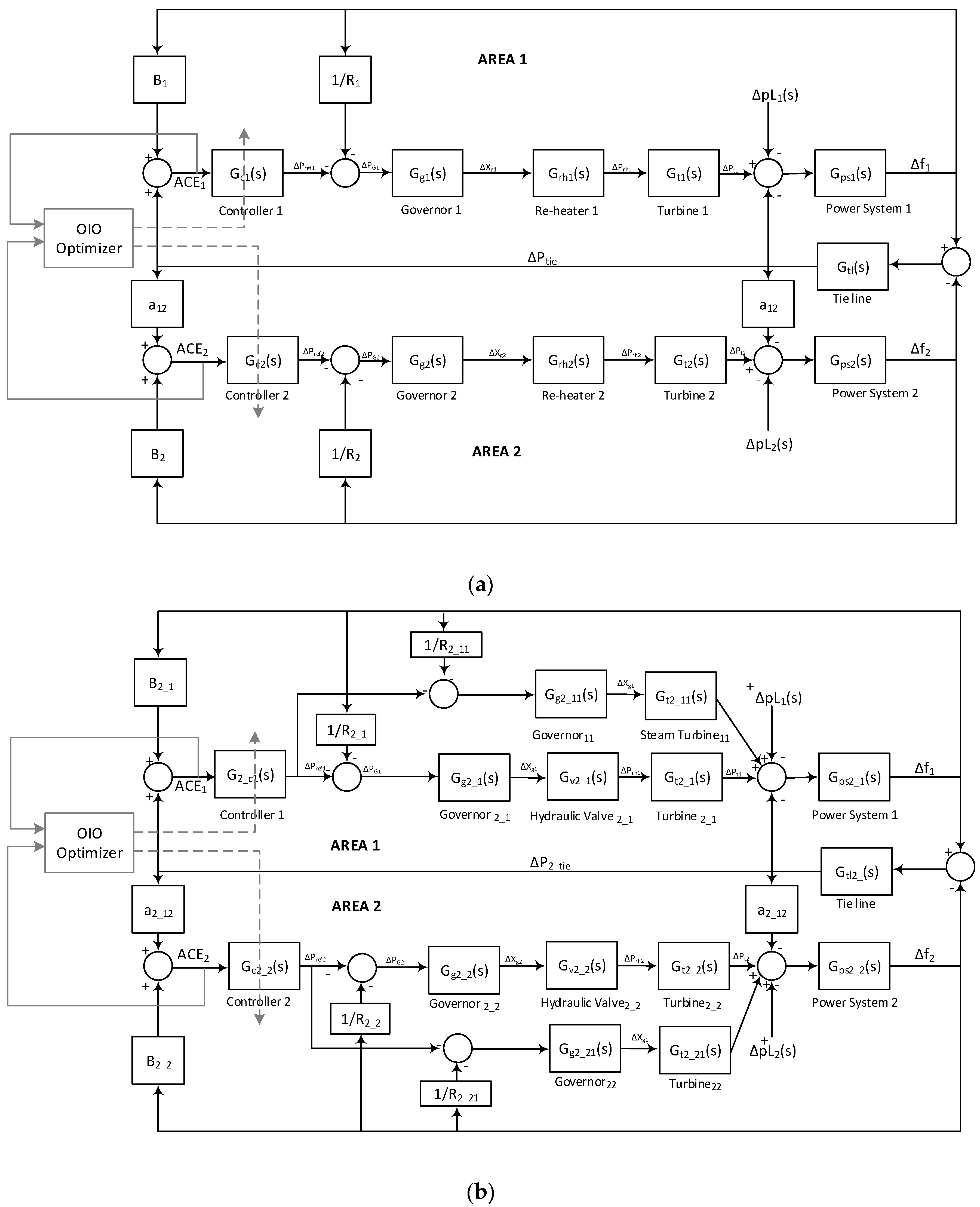

Figure 3.
Change in frequency of area-1 for ITAE.
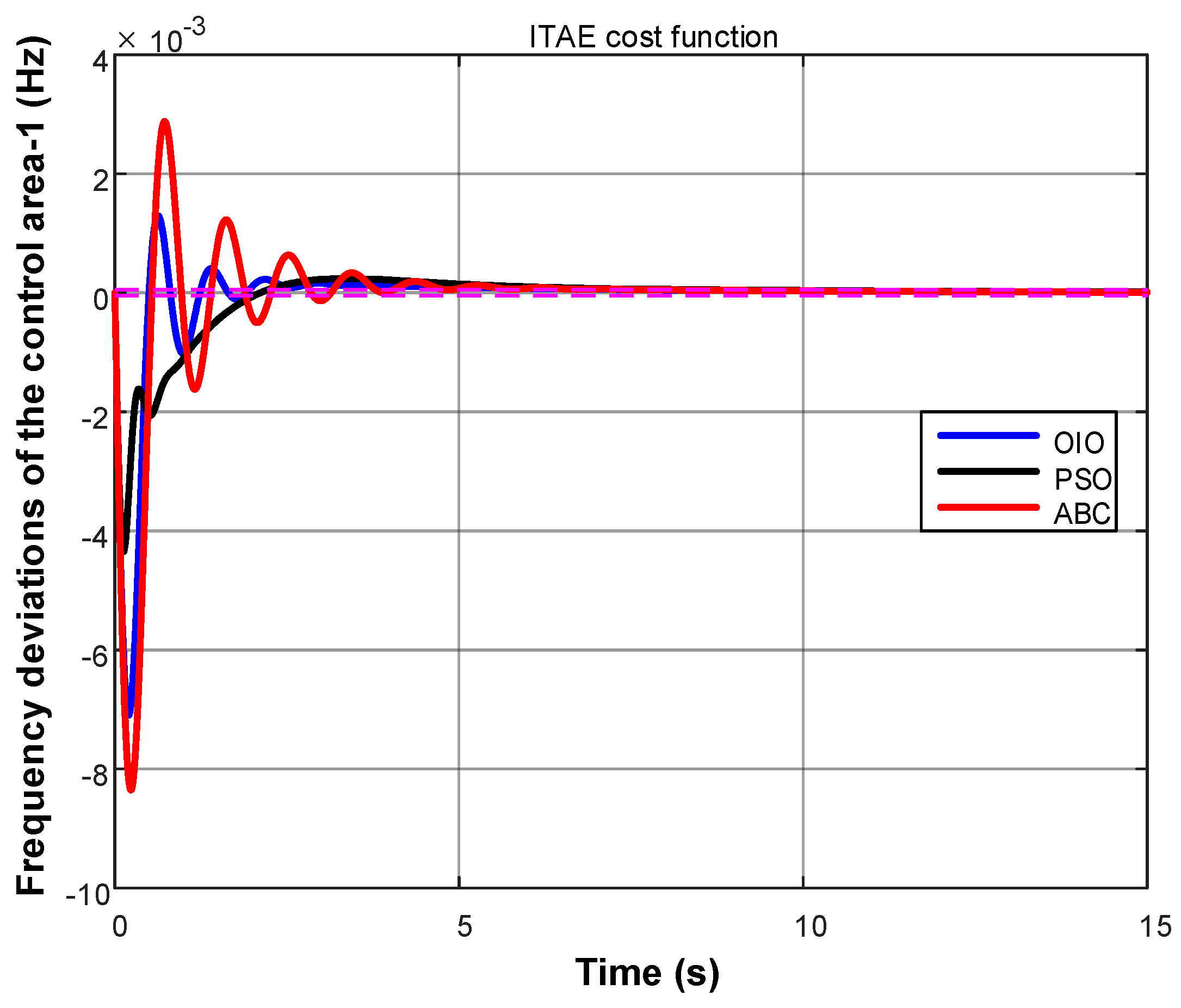
Figure 4.
Change in frequency of area-1 for IAE.

Figure 5.
Change in frequency of area-1 for ISE.
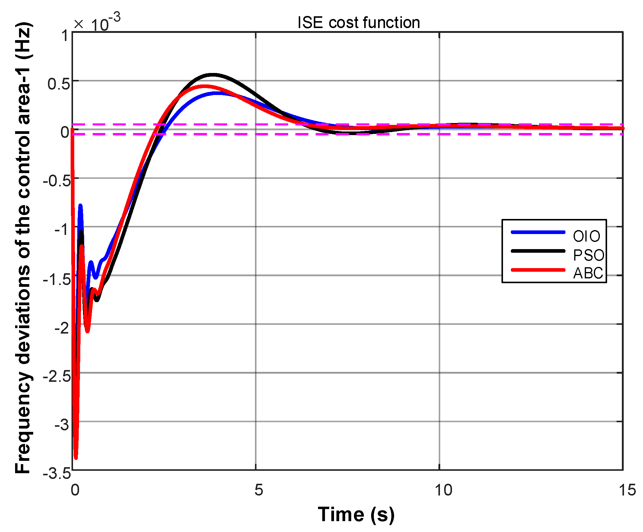
Figure 6.
Change in frequency of area-1 for ITSE.
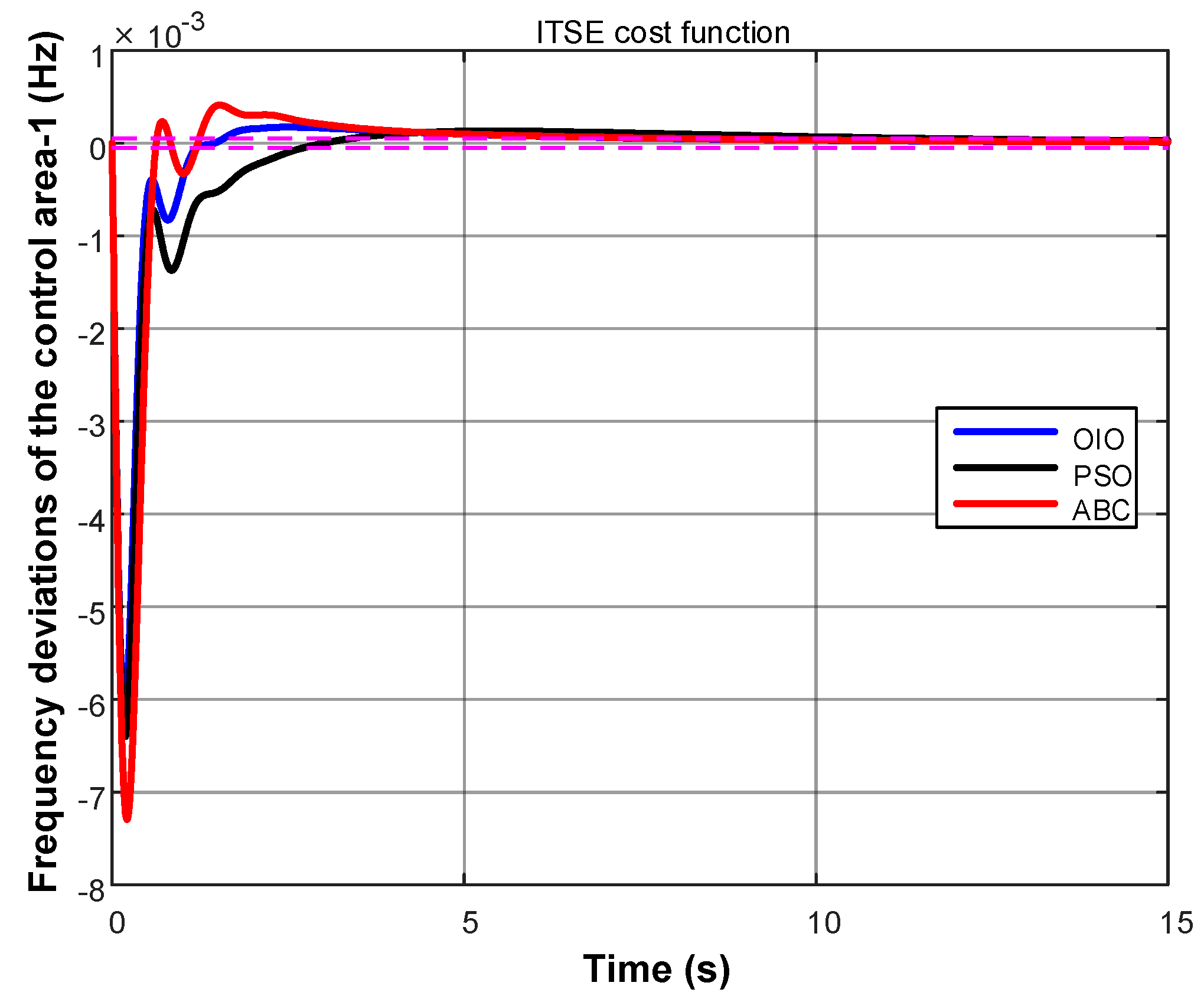
Figure 7.
Change in frequency of area-2 for ITAE.
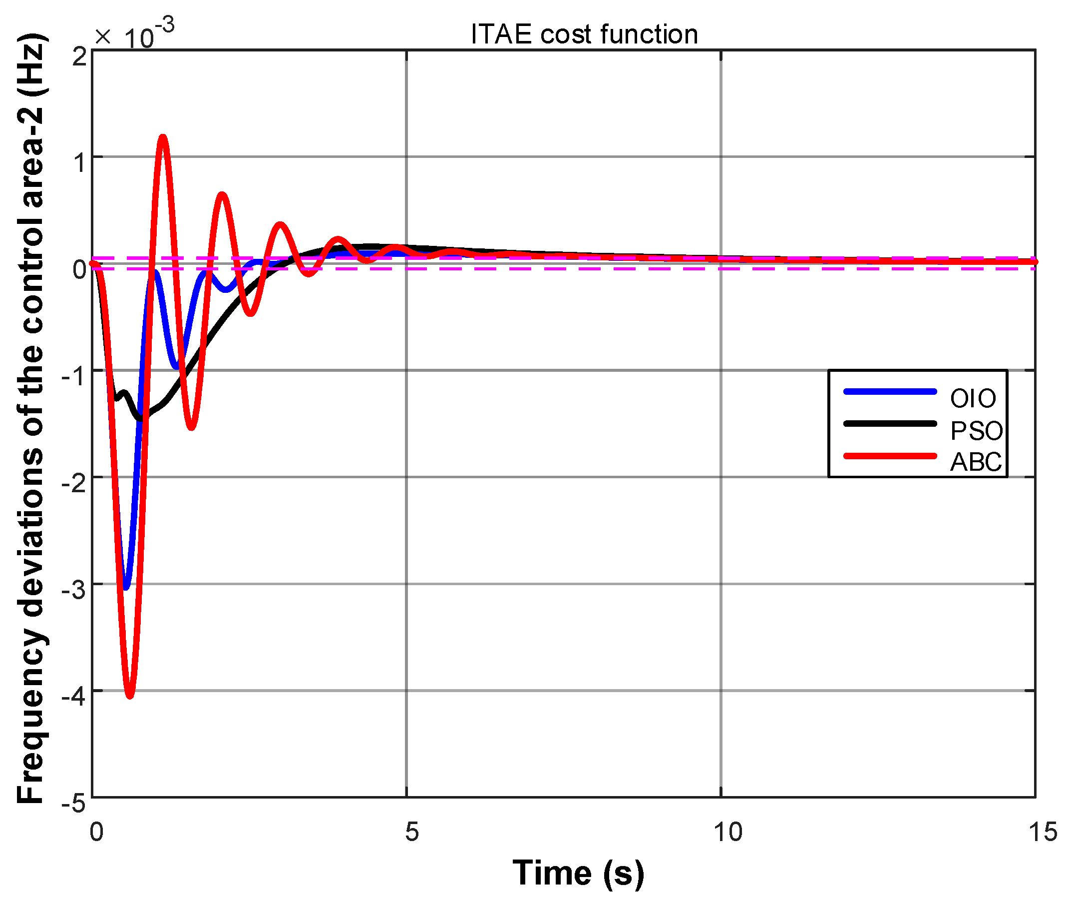
Figure 8.
Change in frequency of area-2 for IAE.

Figure 9.
Change in frequency of area-2 for ISE.

Figure 10.
Change in frequency of area-2 for ITSE.
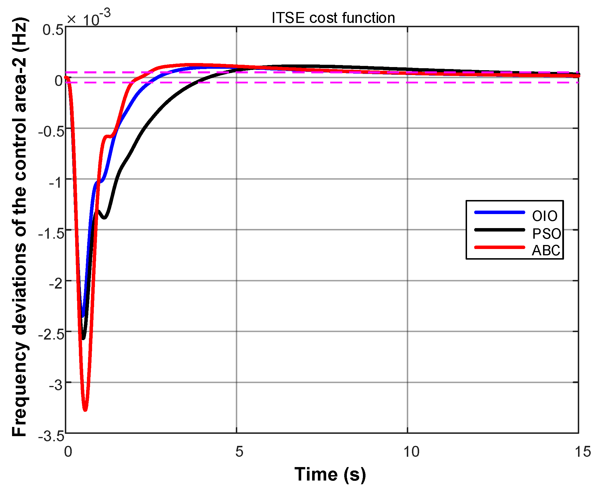
Figure 11.
Change in tie-line power for ITAE.

Figure 12.
Change in tie-line power for IAE.

Figure 13.
Change in tie-line power for ISE.
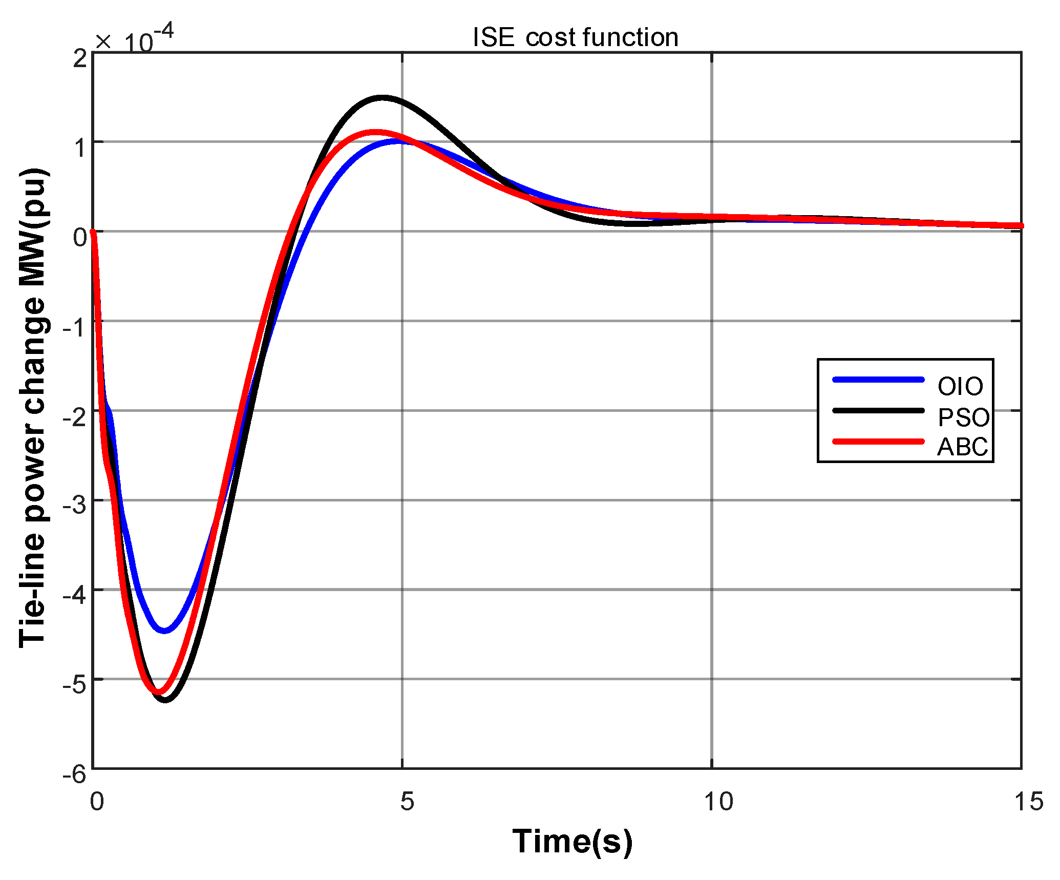
Figure 14.
Change in tie-line power for ITSE.
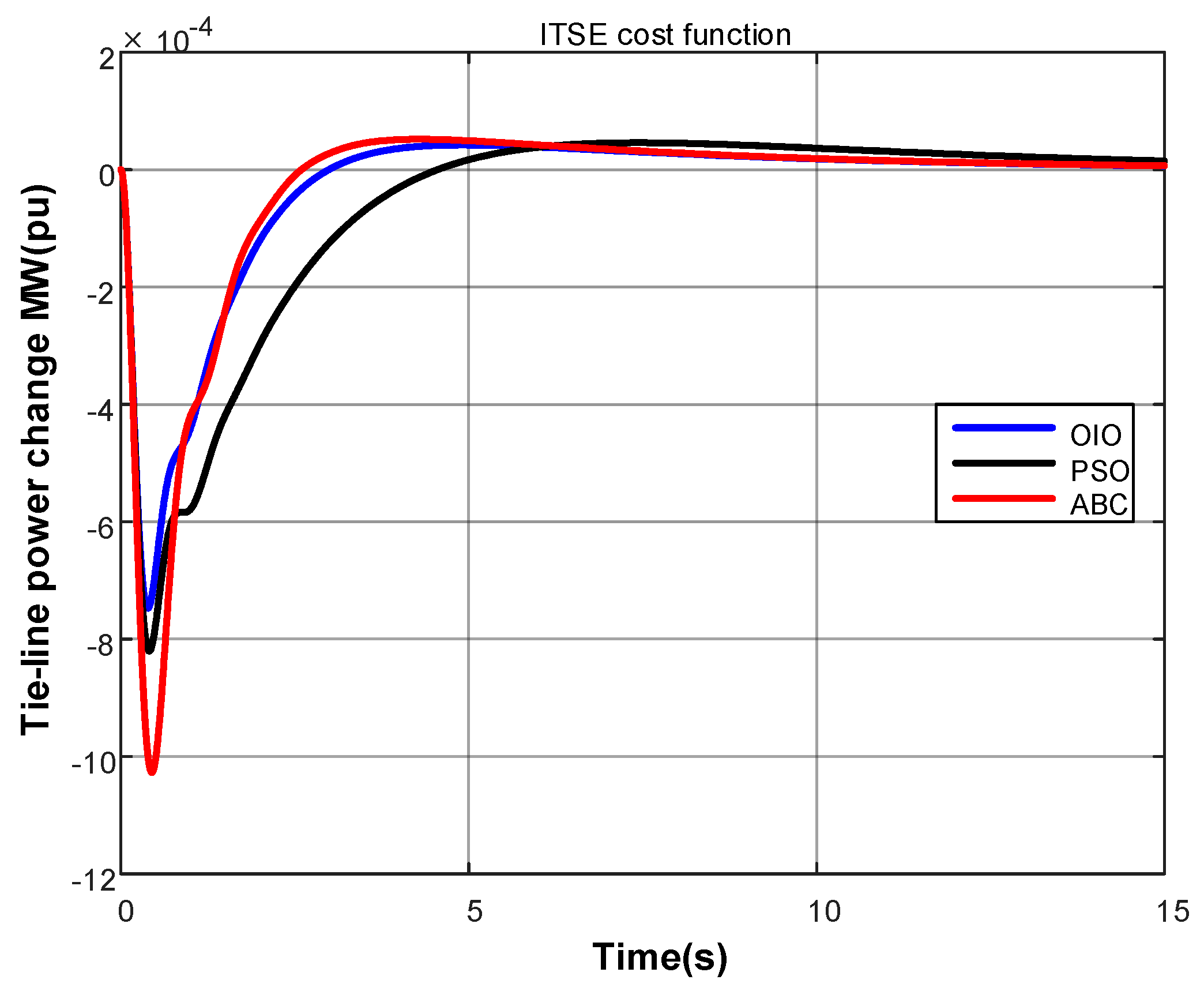
Figure 15.
Iteration history for ITAE.
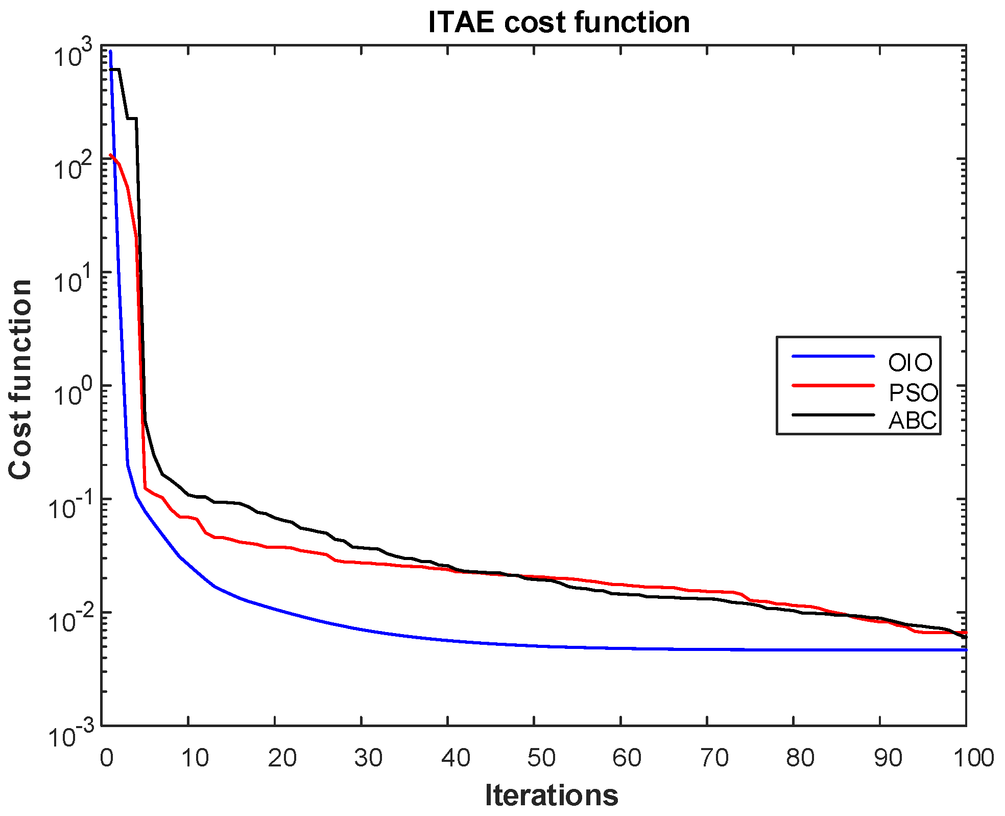
Figure 16.
Iteration history for IAE.
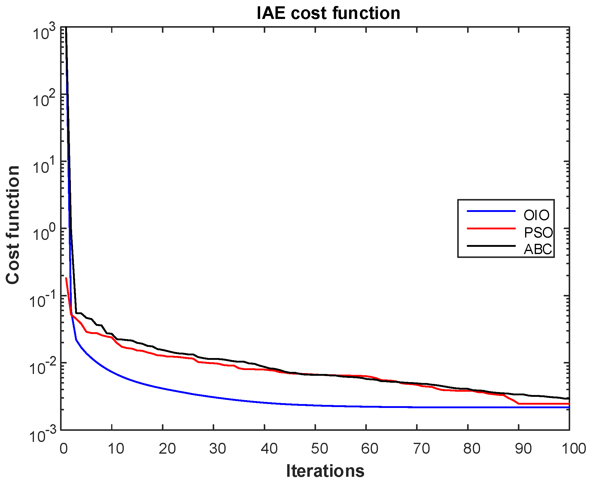
Figure 17.
Iteration history for ISE.
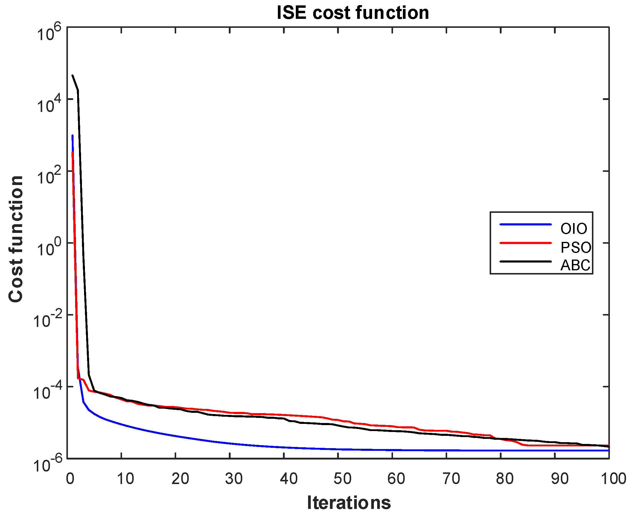
Figure 18.
Iteration history for ITSE.
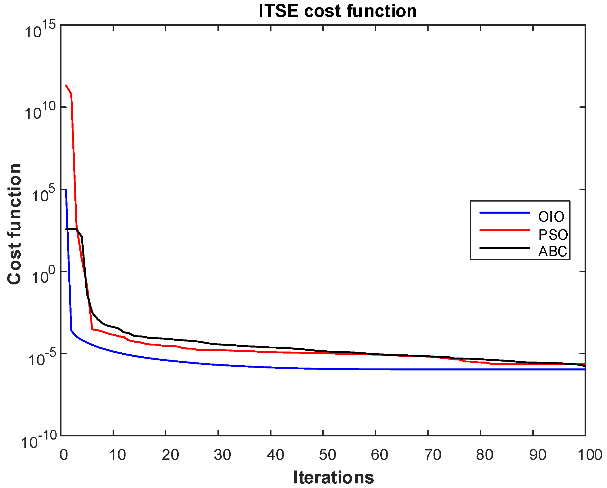
Figure 19.
Iteration history for ITAE.
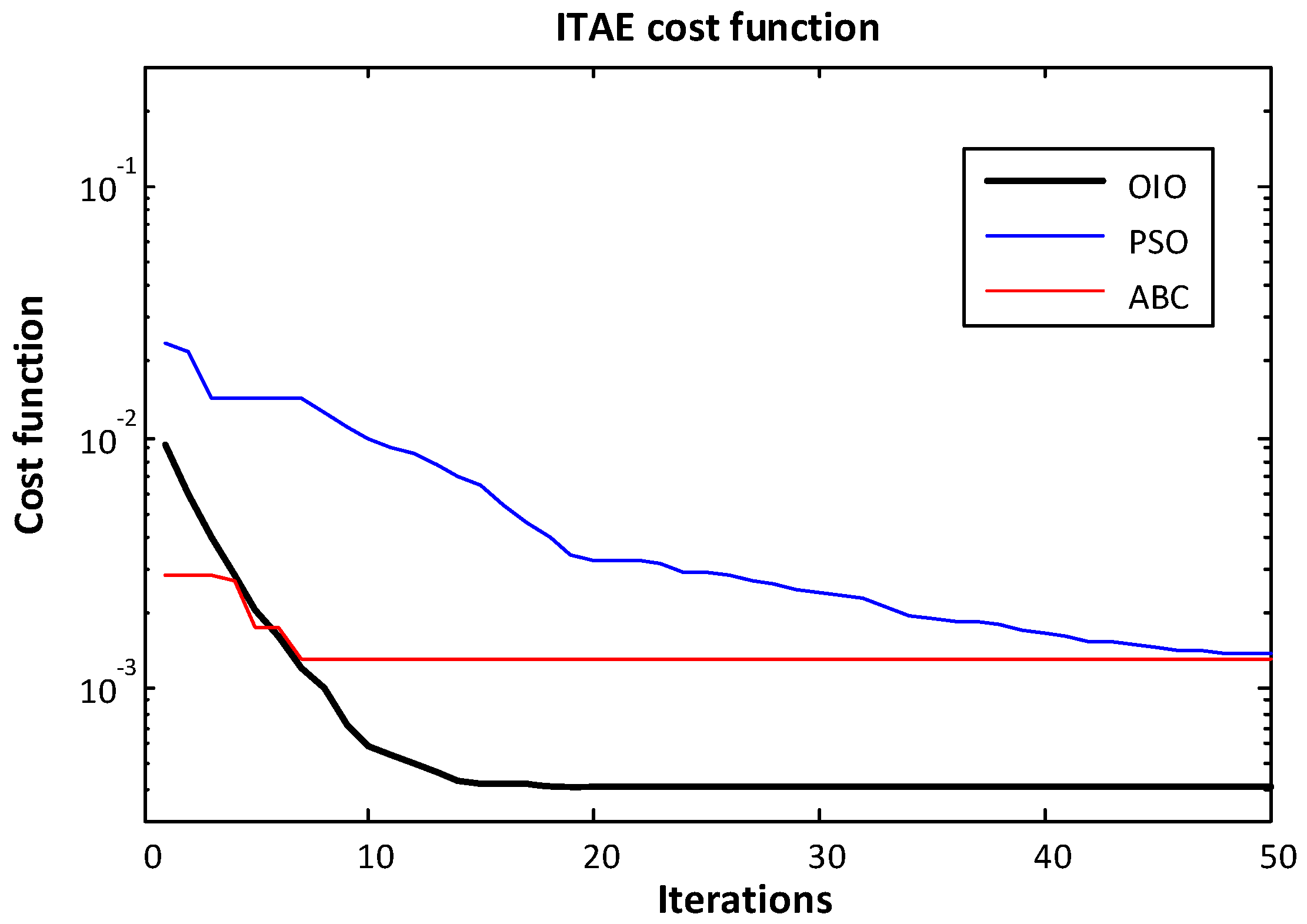
Figure 20.
Iteration history for IAE.

Figure 21.
Iteration history for ISE.

Figure 22.
Iteration history for ITSE.


Table 1.
Limits of Controller Parameters.
| Controller Gain Limits | Kp | Ki | Kd |
|---|---|---|---|
| Upper Limits | 0 | 0 | 0 |
| Lower Limits | 10 | 10 | 10 |
Table 2.
Optimal parameters of the PID controllers for test system-1 and test system-2.
| System | Algoritm | Controller Gains | IAE | ISE | ITSE | ITAE |
|---|---|---|---|---|---|---|
| Test system 1 | OIO | Kp | 9.999 | 9.999 | 9.999 | 9.997 |
| Ki | 9.999 | 9.999 | 9.998 | 9.999 | ||
| Kd | 1.765 | 1.778 | 9.861 | 2.524 | ||
| PSO | Kp | 9.874 | 9.342 | 7.505 | 9.505 | |
| Ki | 8.479 | 8.614 | 9.454 | 5.68 | ||
| Kd | 4.934 | 1.793 | 8.915 | 2.305 | ||
| ABC | Kp | 8.062 | 6.405 | 8.580 | 7.331 | |
| Ki | 9.510 | 9.047 | 9.461 | 9.214 | ||
| Kd | 1.225 | 1.791 | 7.817 | 1.821 | ||
| Test system 2 | OIO | Kp | 5.571 | 4.969 | 4.061 | 4.545 |
| Ki | 5.789 | 3.001 | 3.903 | 2.211 | ||
| Kd | 1.312 | 1.487 | 1.965 | 1.497 | ||
| PSO | Kp | 2.093 | 5.782 | 5.277 | 4.592 | |
| Ki | 7.341 | 9.998 | 1.273 | 7.141 | ||
| Kd | 0.545 | 1.520 | 1.774 | 1.149 | ||
| ABC | Kp | 5.818 | 4.327 | 6.358 | 4.191 | |
| Ki | 1.483 | 3.026 | 9.998 | 7.119 | ||
| Kd | 1.263 | 1.458 | 1.547 | 1.128 |
Table 3.
Settling times and maximum overshoots (max. oversht.) of the frequency deviation of the control area-1.
Table 3.
Settling times and maximum overshoots (max. oversht.) of the frequency deviation of the control area-1.
| System | Algoritm | Step Response | IAE | ISE | ITSE | ITAE |
|---|---|---|---|---|---|---|
| Test system 1 | OIO | Max. oversht. | 7.07 × 10⁻³ | 2.94 × 10⁻³ | 6.09 × 10⁻³ | 7.09 × 10⁻³ |
| Settling times | 8.056390 | 6.860694 | 8.030881 | 8.056704 | ||
| PSO | Max. oversht. | 7.12 × 10⁻³ | 3.14 × 10⁻³ | 6.40 × 10⁻³ | 4.34 × 10⁻³ | |
| Settling times | 8.905854 | 6.310906 | 11.743802 | 8.887682 | ||
| ABC | Max. oversht. | 7.46 × 10⁻³ | 3.37 × 10⁻³ | 7.29 × 10⁻³ | 8.35 × 10⁻³ | |
| Settling times | 8.168429 | 6.364761 | 8.183634 | 8.223559 | ||
| Test system 2 | OIO | Max. oversht. | 2.74 × 10⁻³ | 2.62 × 10⁻³ | 2.35 × 10⁻³ | 2.62 × 10⁻³ |
| Settling times | 1.788248 | 1.996599 | 2.913395 | 1.865132 | ||
| PSO | Max. oversht. | 4.15 × 10⁻³ | 2.59 × 10⁻³ | 2.44 × 10⁻³ | 2.92 × 10⁻³ | |
| Settling times | 1.409041 | 2.447668 | 2.249040 | 2.547392 | ||
| ABC | Max. oversht. | 2.78 × 10⁻³ | 2.65 × 10⁻³ | 2.56 × 10⁻³ | 2.95 × 10⁻³ | |
| Settling times | 1.892082 | 2.25415 | 2.662097 | 2.4863540 |
Table 4.
Settling times and maximum overshoots of the frequency deviation of the control area-2.
| System | Algoritm | Step Response | IAE | ISE | ITSE | ITAE |
|---|---|---|---|---|---|---|
| Test system 1 | OIO | Max. oversht. | 3.02 × 10⁻³ | 1.11 × 10⁻³ | 2.35 × 10⁻³ | 3.04 × 10⁻³ |
| Settling times | 8.934293 | 7.677125 | 8.929580 | 8.934334 | ||
| PSO | Max. oversht. | 3.08 × 10⁻³ | 1.32 × 10⁻³ | 2.57 × 10⁻³ | 1.45 × 10⁻³ | |
| Settling times | 9.801351 | 6.999126 | 12.630685 | 9.904835 | ||
| ABC | Max. oversht. | 3.45 × 10⁻³ | 1.29 × 10⁻³ | 3.27 × 10⁻³ | 4.05 × 10⁻³ | |
| Settling times | 9.111831 | 7.201539 | 9.121439 | 8.941476 | ||
| Test system 2 | OIO | Max. oversht. | 9.77 × 10⁻⁵ | 8.79 × 10⁻⁵ | 8.30 × 10⁻⁵ | 9.50 × 10⁻⁵ |
| Settling times | 3.939263 | 5.523281 | 4.862744 | 5.94255 | ||
| PSO | Max. oversht. | 2.75 × 10⁻⁴ | 1.13 × 10⁻⁴ | 1.09 × 10⁻⁴ | 1.32 × 10⁻⁴ | |
| Settling times | 6.158258 | 7.257616 | 6.807813 | 7.61831 | ||
| ABC | Max. oversht. | 1.09 × 10⁻⁴ | 9.04 × 10⁻⁵ | 1.14 × 10⁻⁴ | 1.34 × 10⁻⁴ | |
| Settling times | 6.573563 | 5.447564 | 7.339555 | 7.529223 |
Table 5.
Value of cost function for OIO, PSO, and ABC.
| System | Algoritm | IAE | ISE | ITSE | ITAE |
|---|---|---|---|---|---|
| Test system 1 | OIO | 2.16 × 10⁻³ | 1.68 × 10⁻⁶ | 1.05 × 10⁻⁶ | 4.67 × 10⁻³ |
| PSO | 2.46 × 10⁻³ | 2.34 × 10⁻⁶ | 2.29 × 10⁻⁶ | 6.65 × 10⁻³ | |
| ABC | 2.78 × 10⁻³ | 2.12 × 10⁻⁶ | 1.59 × 10⁻⁶ | 5.56 × 10⁻³ | |
| Test system 2 | OIO | 7.22 × 10⁻⁴ | 6.80 × 10⁻⁷ | 1.50 × 10⁻⁷ | 2.16 × 10⁻³ |
| PSO | 8.75 × 10⁻⁴ | 7.40 × 10⁻⁷ | 1.90 × 10⁻⁷ | 2.46 × 10⁻³ | |
| ABC | 7.59 × 10⁻⁴ | 8.40 × 10⁻⁷ | 2.00 × 10⁻⁷ | 2.78 × 10⁻³ |
Table 6.
Total computation time table in second.
| System | Algoritm | IAE | ISE | ITSE | ITAE |
|---|---|---|---|---|---|
| Test system 1 | OIO | 389.5745 | 391.4756 | 391.1157 | 389.4153 |
| PSO | 497.208 | 489.2443 | 477.7997 | 492.3465 | |
| ABC | 552.9799 | 559.9015 | 553.7232 | 560.1486 | |
| Test system 2 | OIO | 199.1631 | 198.4873 | 197.0914 | 195.9271 |
| PSO | 249.3927 | 243.8966 | 243.0222 | 250.9786 | |
| ABC | 277.4441 | 280.5757 | 278.4784 | 281.0236 |
© 2017 by the authors. Licensee MDPI, Basel, Switzerland. This article is an open access article distributed under the terms and conditions of the Creative Commons Attribution (CC BY) license (http://creativecommons.org/licenses/by/4.0/).
Share and Cite
MDPI and ACS Style
ÖZDEMİR, M.T.; ÖZTÜRK, D. Comparative Performance Analysis of Optimal PID Parameters Tuning Based on the Optics Inspired Optimization Methods for Automatic Generation Control. Energies 2017, 10, 2134. https://doi.org/10.3390/en10122134
AMA Style
ÖZDEMİR MT, ÖZTÜRK D. Comparative Performance Analysis of Optimal PID Parameters Tuning Based on the Optics Inspired Optimization Methods for Automatic Generation Control. Energies. 2017; 10(12):2134. https://doi.org/10.3390/en10122134
Chicago/Turabian StyleÖZDEMİR, Mahmut Temel, and Dursun ÖZTÜRK. 2017. "Comparative Performance Analysis of Optimal PID Parameters Tuning Based on the Optics Inspired Optimization Methods for Automatic Generation Control" Energies 10, no. 12: 2134. https://doi.org/10.3390/en10122134
Note that from the first issue of 2016, this journal uses article numbers instead of page numbers. See further details here.